Publisher’s version / Version de l'éditeur:
PERD/CHC Report 5-91, 1998-03
READ THESE TERMS AND CONDITIONS CAREFULLY BEFORE USING THIS WEBSITE. https://nrc-publications.canada.ca/eng/copyright
Vous avez des questions? Nous pouvons vous aider. Pour communiquer directement avec un auteur, consultez la
première page de la revue dans laquelle son article a été publié afin de trouver ses coordonnées. Si vous n’arrivez pas à les repérer, communiquez avec nous à [email protected].
Questions? Contact the NRC Publications Archive team at
[email protected]. If you wish to email the authors directly, please see the first page of the publication for their contact information.
Archives des publications du CNRC
For the publisher’s version, please access the DOI link below./ Pour consulter la version de l’éditeur, utilisez le lien DOI ci-dessous.
https://doi.org/10.4224/12327797
Access and use of this website and the material on it are subject to the Terms and Conditions set forth at Investigation of Techniques for Continuously Profiling Ice Features Comfort, G.
https://publications-cnrc.canada.ca/fra/droits
L’accès à ce site Web et l’utilisation de son contenu sont assujettis aux conditions présentées dans le site LISEZ CES CONDITIONS ATTENTIVEMENT AVANT D’UTILISER CE SITE WEB.
NRC Publications Record / Notice d'Archives des publications de CNRC:
https://nrc-publications.canada.ca/eng/view/object/?id=079742e6-b115-4728-a1c8-acb0570d5be6 https://publications-cnrc.canada.ca/fra/voir/objet/?id=079742e6-b115-4728-a1c8-acb0570d5be6
INVESTIGATION OF
TECHNIQUES FOR CONTINUOUSLY PROFILING ICE FEATURES
G. Comfort
Submitted to: Attn: Dr G. Timco Canadian Hydraulics Centre National Research Council Canada
Montreal Road, Bldg. M-32 Ottawa, Ontario
K1A OR6
Submitted by: Fleet Technology Limited
311 Legget Drive Kanata, Ontario
K2K 1Z8
DISCLAIMER
The views expressed in this report are those of Fleet Technology Ltd. and do not necessarily represent those of the Government of Canada.
Efforts have been made to the extent possible to avoid naming commercial suppliers or products in this report. Any commercial suppliers or products named in this report are done so only to provide added information, and this does not constitute an endorsement on our part.
Furthermore, it should be noted that this project was not intended to produce a catalogue of the available equipment and suppliers. However, recognizing that the available equipment is an important aspect of the work, a compendium of sample brochures and equipment descriptions has been assembled and prepared. These have been submitted to the National Research Council under separate cover, as an Annex to this report,. The inclusion or exclusion of a particular supplier or product in this Annex constitutes neither an endorsement nor a negative recommendation on Fleet Technology Ltd.’s part.
Fleet Technology Limited Internal Review :
Approved For Release By : Date :
EXECUTIVE SUMMARY
The techniques used to date for profiling ice ridges, hummock fields and icebergs have been reviewed and summarized. For ridges, the past techniques fall into two categories : (a) bottom-mounted systems ; and : (b) mobile systems. For icebergs, the past techniques fall into the following categories : (a) inferences from sail observations ; and : (b) direct underwater measurements. The requirements for under-ice data have been reviewed and analyzed, as summarized below :
• Ridges And Hummock Fields :
(a) three-dimensional data are required to define the maximum keel depth to acceptable precision.
(b) two-dimensional data will provide a reasonable definition of the underwater volume of a hummock field.
• Icebergs :
(a) it is necessary to measure the keel portion of the iceberg. Keel parameters inferred from sail observations are only of first order.
(b) the iceberg shape is a very important parameter affecting the loads on a structure, and projects undertaken with this end objective should include measurements of the iceberg shape.
The available technology for profiling ridges and hummock fields is relatively well-developed. The most significant technology improvements since the most recent profiling projects are believed to be with respect to :
(a) platforms - Although some past profiling projects have been conducted using Remotely Operated Vehicles (ROVs), it is noted that ROVs and Autonomous Underwater Vehicles (AUVs) have developed further.
(b) sensor technology - multi-beam sonars have developed further with the result that they have become easier to use (i.e., smaller and lighter) and more affordable. Although profiling projects have not been conducted using all of these technology
improvements, this application is believed to be relatively well-served.
However, the available technology for profiling icebergs is less well-developed, partly because this is a more difficult problem (than ridges and hummock fields), and partly because iceberg profiling projects have not been conducted recently. The technology
TABLE OF CONTENTS
Page
1.0 INTRODUCTION AND OBJECTIVES 1
2.0 DATA COLLECTION REQUIREMENTS 3
2.1 Motivations For Data Collection 3 2.2 Information Content Comparison : Two-Dimensional Versus 4
Three-Dimensional Data
2.3 Information Requirements From Under-Ice Surveys 13 3.0 TECHNIQUES USED TO DATE FOR ENVIRONMENT DEFINITION 18
STUDIES OF ICE RIDGES AND HUMMOCK FIELDS
3.1 Overview 18
3.2 Bottom-Mounted, Upward-Looking Fixed Installations 18
3.3 Mobile Systems : Overview 21
3.4 Mobile Systems Deployed From Below The Ice Surface 21 3.5 Mobile Systems Deployed Through A Hole In The Ice Sheet 22 3.6 Mobile Systems Deployed From Above Or On The Ice Surface 25 4.0 TECHNIQUES USED TO DATE FOR ENVIRONMENT DEFINITION 26
STUDIES OF ICEBERGS
4.1 General 26
4.2 Above-Water Techniques 27
4.3 Below-Water Techniques 28
5.0 TECHNIQUES USED TO DATE FOR OPERATIONAL MONITORING 34 5.1 Application : Ice Discharge Monitoring In The St. Lawrence River 34 5.2 Application : Monitoring Of Ice Conditions At The Niagara 36
Power Project’s Water Intakes
5.3 Application : Route Selection For Icebreakers And Ships 36 Operating In Ice In The Gulf of St. Lawrence
5.4 Application : Iceberg Draft At The Hibernia Structure 37 6.0 THE PRESENT STATE-OF-THE-ART AND RECOMMENDATIONS 38 6.1 Ice Features Of Interest : Ridges And Hummock Fields 38 6.2 Ice Features Of Interest : Icebergs 43
7.0 CONCLUSIONS AND RECOMMENDATIONS 48
TABLE OF CONTENTS (cont’d)
APPENDICES :
APPENDIX A - Quantitative Analysis Of Multi-Year Floe Parameters Using Field Measurements Of Above-Ice And Under-Ice Topography
ANNEX (under separate cover) :
Investigation Of Techniques For Continuously Profiling Ice Features : Annex Of Equipment Brochures
LIST OF FIGURES
Page
Figure 2.1 Sample Result : Effect Of Line Spacing On Maximum Sail Height 6
Figure 2.2 Sample Result : Effect Of Line Spacing On Maximum Keel Depth 6
Figure 2.3 Sample Result : Effect Of Line Spacing On Under-Ice Volume 7
Figure 2.4 Sample Result : Effect Of Line Spacing On Maximum Sail Height 7
Figure 2.5 Sample Result : Effect Of Line Spacing On Maximum Keel Depth 12
Figure 2.6 Sample Result : Effect Of Line Spacing On Under-Ice Volume 12
Figure 2.7 Iceberg Interaction With A Stepped Steel Gravity Platform 15
Figure 2.8 Iceberg With “Underwater Rams” 17
Figure 3.1 Techniques Used To Date 19
Figure 3.2 Sonar Deployments From The Ice Surface 23
Figure 4.1 Maximum Draft System Used By Robe, 1975 29
Figure 4.2 System Used To Measure Iceberg Shape And Draft : 31
Sonar Transducer Position Referenced To Survey Vessel Figure 4.3 System Used To Measure Iceberg Shape And Draft : 32
Sonar Transducer Position Referenced To Transponders On The Iceberg Figure 6.1 Proposed Systems For Measuring Iceberg Shape 46
LIST OF TABLES
Page Table 1.1 Cases Where Under-Ice Topographic Data Are Useful 2 Table 2.1 Sources Of Three-Dimensional Under-Ice Topographic Data 4 Table 2.2 Summary Results : Quantitative Analyses Of The Multi-Year Floe 8
Field Data Collected By Harrington And St. John, 1987
Table 2.3 Summary Results : Quantitative Analyses Of The Multi-Year Floe 11 Field Data Collected By Melling, Topham, and Reidel, 1993
Table 2.4 Information Requirements From Under-ice Surveys 13 Table 3.1 Bottom-Mounted, Upward-Looking Fixed Installations 18 Table 3.2 Mobile Systems : Deployment Surface & Measurement Methods 21 Table 4.1 Summary Of Above-Water Profiling Techniques Used To Date 26
For Icebergs
Table 4.2 Summary Of Below-Water Profiling Techniques Used To Date 27 For Icebergs
Table 5.1 Operational Monitoring Applications and Systems Used 34 Table 6.1 Profiling Ridges And Hummock Fields : General Cases Of Interest 38 Table 6.2 Profiling Methods For Environment Definition Surveys : 39
Draft Of Ridge Keels And Hummock Fields
Table 6.3 Profiling Methods For Environment Definition Surveys : 41 Shape And Volume Of Ridge Keels And Hummock Fields
Table 6.4 Profiling Methods For Operational Monitoring : 42 Draft Of Ridge Keels And Hummock Fields
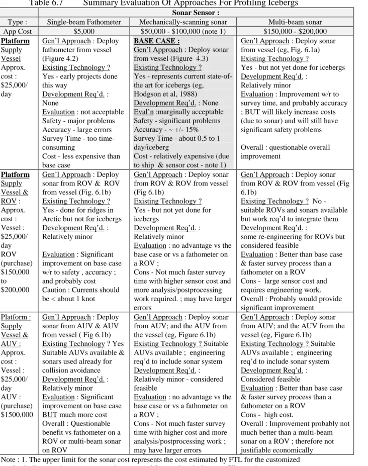
Table 6.5 Profiling Icebergs : General Cases Of Interest 43 Table 6.6 Recommended Survey Methods For Iceberg Draft 43 Table 6.7 Summary Evaluation Of Approaches For Profiling Icebergs 45
1.0 INTRODUCTION AND OBJECTIVES
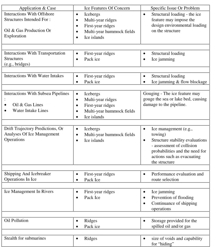
A knowledge of the under-ice surface topography is required to evaluate many cases of practical concern, some of which are listed in Table 1.1.
Often, the collection of this field data is a difficult task that involves significant resources and time. Part of this difficulty stems from the fact that ice features such as ridges, icebergs, or hummock fields can vary significantly, and hence, a large number of
measurements are required to quantify them in a meaningful way. Ideally, this database should be collected over several years. However, this is usually not possible because decisions to explore and subsequently develop an area (e.g., for oil & gas deposits) are often made on relatively short time scales. In these cases, the oil company, upon entering a new area, is faced with the task of acquiring environmental information in a relatively short time to allow exploration and development decisions to be made. In these cases, the ideal system(s) would allow the oil company to enter a new area, and acquire a large amount of data quickly.
Difficulties are also imposed by practical and logistical issues. The majority of these features are below the waterline, which makes them difficult to access. Furthermore, the ice features of interest are usually located in remote regions.
A great deal of effort has been expended over the past three decades to acquire data to define the under-ice profile and topography of ice features of concern. As developments in ice-covered regions continue, methods for acquiring under-ice data are an area of ongoing interest.
The objectives of this project were to :
(a) review the requirements for under-ice topographic data.
(b) document methods previously used to obtain under-ice topographic data, and subsequent technology changes.
(c) make recommendations for profiling methods.
It should be noted that while a large part of the work involved reviewing the available technology, the project was not intended to produce a catalogue of the available
equipment. However, recognizing that the available equipment is an important aspect of the work, a compendium of sample brochures and equipment descriptions has been assembled and prepared. These have been submitted under separate cover, as Annex A.
Table 1.1 Cases Where Under-Ice Topographic Data Are Useful
Application & Case Ice Features Of Concern Specific Issue Or Problem Interactions With Offshore
Structures Intended For : Oil & Gas Production Or Exploration
• Icebergs
• Multi-year ridges
• First-year ridges
• Multi-year hummock fields
• Ice islands
• Structural loading - the ice feature may impose the design environmental loading on the structure
Interactions With Transportation Structures (e.g., bridges) • First-year ridges • Pack ice • Structural loading • Ice jamming Interactions With Water Intakes • First-year ridges
• Pack ice
• Structural loading
• Ice jamming & flow blockage Interactions With Subsea Pipelines
:
• Oil & Gas Lines
• Water Intake Lines
• Icebergs
• Multi-year ridges
• First-year ridges
• Multi-year hummock fields
• Ice islands
Gouging - The ice feature may gouge the sea or lake bed, causing damage to the pipeline.
Drift Trajectory Predictions, Or Analyses Of Ice Management Operations
• Icebergs
• Multi-year hummock fields
• Ice islands
• Ice management (e.g., towing)
• Structure stability evaluations - assessment of collision probabilities and the need for actions such as evacuating the structure
Shipping And Icebreaker Operations In Ice
• First-year ridges
• Pack Ice
• Performance evaluation and route selection
Ice Management In Rivers • First-year ridges
• Pack Ice
• Ice jamming
• Prevention of flooding
• Continuance of shipping operations
Oil Pollution • Ridges
• Pack ice
• Storage provided for the spilled oil and/or gas Stealth for submarines • Ridges • size of voids and capability
2.0 DATA COLLECTION REQUIREMENTS 2.1 Motivations For Data Collection
The motivations for data collection can be broadly classified into the following two categories :
• Environment Definition - In this case, the under-ice data are principally required to build up a database in support of design or analysis efforts. The cases that fall into this class include :
(a) the design of offshore structures for oil & gas production or exploration ; transportation (e.g., bridges) ; or for water intake.
(b) performance evaluations for offshore structures (e.g., with respect to jamming and flow blockage for water intakes ; ice jamming produced by bridges, etc.). (c) evaluations of the required burial depth for offshore pipelines.
(d) strategic evaluations of pollution problems (e.g., oil spills).
For this case, the primary focus of the data collection efforts is to build up an accurate database that is sufficiently extensive to allow reliable design or analysis decisions to be made. Time is usually of the essence as well because often, the operator is faced with making decisions relatively quickly which precludes longterm monitoring over many years. However, real-time information is not required in this situation. The ideal system(s) for this case is one(s) that would allow an operator to enter the area(s) of interest ; and profile a large number of ice features quickly. Depending on the case of interest, it may be desirable for the operator to be able to select which ice features are to be sampled, versus obtaining a long profile data track.
• Operational Monitoring - In this case, the under-ice data are used to support field operations. The cases that fall into this class include :
(a) ice discharge measurements in rivers (e.g., to guide ice management efforts such as icebreaker deployments or hydro-electric discharges for controlled rivers). (b) ice monitoring at hydro-electric water intakes (e.g., to assist decision-making regarding ice management operations affecting flow into the intake).
(c) tactical route selection for ship operations.
(d) tactical pollution clean-up efforts (e.g., oil spills).
(e) evaluations of ice management operations and offshore structure stability decisions (e.g., towing , whether or not to evacuate the structure, etc.).
For the Operational Monitoring Case, data collection needs to be done in real-time, and focussed on the specific ice feature(s) of concern at the time.
2.2 Information Content Comparison : Two-Dimensional Versus Three-Dimensional Data
It is obvious that two-dimensional data are considerably simpler to acquire than are three-dimensional data, and, as expected, the majority of the information in the literature to define large ice features consist of profile data. Only a few projects have been carried out to obtain three-dimensional under-ice data, most of which are summarized in Table 2.1.
Table 2.1
Sources Of Three-Dimensional Under-Ice Topographic Data
Ice Feature Project Description Reference
Multi-Year Floes With Hummocks and Ridges
The above-ice and under-ice topography of 7 multi-year floes in the Chukchi Sea were mapped. The size of the mapped area was about 100-150 m by 100-150 m for each floe.
Harrington and St. John, 1987
Multi-Year Hummock Field
The above-ice and under-ice topography of 1 multi-year floe in the Canadian Beaufort Sea was mapped. The size of the mapped area was about 325 m by 300 m.
Melling, Topham and Reidel, 1993
First-Year Ridge In The Canadian Beaufort Sea
The above-ice and under-ice topography of a 300 m long section of one ridge was mapped. The width of the mapped area was about 150 m.
Bowen, and Topham, 1996
Icebergs The Dynamic Ice Grounding Study (DIGS) Four icebergs offshore of Newfoundland were mapped.
Hodgson et al, 1988 No. Of Icebergs Surveyed : 33
Location : Offshore Nfld. (Grand Banks)
Anderson et al, 1984 No. Of Icebergs Surveyed : 4
Location : Offshore Nfld. (Grand Banks)
Ice Eng.Ltd. , 1985 ; Smith et al, 1987 No. Of Icebergs Surveyed : 8
Location : Offshore Nfld. (Grand Banks)
Ice Eng.Ltd. , 1984 ; Smith et al, 1987 No. Of Icebergs Surveyed : 6
Location : Offshore Nfld. (Strait Of Belle Isle)
Ice Eng.Ltd. , 1983 ; Smith et al, 1987
The field data collected by Harrington and St. John, 1987, and by Melling, Topham, and Reidel, 1993 were analyzed to compare the information content of two-dimensional versus three-dimensional data. These data sets were selected for analysis because the ice features surveyed were primarily areal in extent (as opposed to being essentially linear, such as a ridge). Three-dimensional data are expected to add the greatest information content (compared to two-dimensional data) for this type of ice feature.
The analyses were conducted with respect to the following parameters : (a) the maximum sail height ;
They surveyed the above-ice and below-ice topography of 7 large multi-year floes in the Chukchi Sea. The mapped areas for each floe ranged from 66 m x 56 m to 210 m x 95 m. Under-ice topographic data were collected using two methods : (a) an upward-looking sonar mounted on a Remotely Operated Vehicle (ROV) ; and (b) a sonar system that was lowered beneath the ice on lowering rods, with the sonar transducer being rotated through various angles (which they termed the IMAPS System). Only the IMAPS data were used for the analyses conducted here, because Harrington and St. John, 1987 found that the ice drafts measured using the ROV did not correlate well with the measurements made by direct drilling. They attributed this to positioning errors for the ROV. It should be noted that this lack of correlation is not indicative of present-day ROV technology because significant improvements have been made since Harrington and St. John, 1987’s surveys were carried out.
The work was conducted by analyzing cross-sections drawn at various line spacings through the contour maps prepared by Harrington and St.John, 1987.
Figures 2.1 and 2.2 show sample comparisons of the maximum sail height, and keel depth for various line spacings. A full set of all plots is provided in Appendix A. Table 2.2 summarizes the results. Because there is always a chance that one possible line spacing case will include the line that contains the maximum sail height or keel depth, the upper bound of the range of variation for these parameters is zero (i.e., the maximum is included and sampled) for all line spacings considered. However, as the study area is sampled less (i.e. at wider line spacings), the chance that the maximum value will be included becomes reduced, and most likely the survey will underestimate the actual maximum sail height or keel depth. The analyses show that in order to limit the
maximum possible discrepancy to 10 % to of the maximum value for the sail height and keel depth, the line spacing should be no more than about 10 m (30 ft). See Table 2.2. Figure 2.3 shows how the under-ice volume is affected by the survey line spacing, and these results are summarized in Table 2.2. The relationship between the calculated under-ice volume and the line spacing depends on the irregularity of the under-ice surface and where the selected survey lines happen to be located. Thus, the under-ice volume may be either over-estimated or under-estimated by sampling the study area less (i.e., at wider line spacings), as shown in Table 2.2. The analyses show that the under-ice volume is more likely to be over-estimated than under-estimated by sampling the study area less (i.e., at wider line spacings). In order to limit the maximum possible discrepancy to + 3 % and - 3 % of the maximum value for the under-ice volume, the line spacing should be no more than about 15.2 m (50 ft), and 10 m (30 ft), respectively. See Table 2.2.
Figure 2.1 Sample Result : Effect Of Line Spacing On Maximum Sail Height Error! Not a valid link.
Figure 2.2 Sample Result : Effect Of Line Spacing On Maximum Keel Depth Error! Not a valid link.
Figure 2.3 Sample Result : Effect Of Line Spacing On Under-Ice Volume Error! Not a valid link.
Figure 2.4 Sample Result : Effect Of Line Spacing On Maximum Sail Height Error! Not a valid link.
Table 2.2
Summary Results : Quantitative Analyses Of The Multi-Year Floe Field Data Collected By Harrington And St. John, 1987
Parameter
“Maximum” Value Definition Basis And Value
Average Range Of Variation (%) For All Sites Analyzed Compared To The Maximum Value :
Based On Maximum Line Upper Lower
Line Spacing Of Value Spacing Bound Bound
Sail 3.1 m (10 ft) Site 1: 4.0 6.2 m (20 ft) 0 -7.5 Height 3.1 m (10 ft) Site 2 : 3.0 9.3 m (30 ft) 0 -10.7 (m) 3.1 m (10 ft) Site 3 : 3.0 12.2 m (40 ft) 0 -15.2 3.1 m (10 ft) Site 4 : 4.3 15.2 m (50 ft) 0 -19.5 3.1 m (10 ft) Site 5 : 3.0 18.3 m (60 ft) 0 -20.9 3.1 m (10 ft) Site 7 : 4.0 Keel 3.1 m (10 ft) Site 1: 14.8 6.2 m (20 ft) 0 -6.7 Depth 3.1 m (10 ft) Site 2 : 7.3 9.3 m (30 ft) 0 -8.6 (m) 3.1 m (10 ft) Site 3 : 6.7 12.2 m (40 ft) 0 -14.8 3.1 m (10 ft) Site 4 : 12.2 15.2 m (50 ft) 0 -18.5 3.1 m (10 ft) Site 5 : 10.4 18.3 m (60 ft) 0 -21.9 3.1 m (10 ft) Site 6 : 11.0 3.1 m (10 ft) Site 7 : 15.8 Under-Ice 3.1 m (10 ft) Site 4 : 6.2 m (20 ft) 0 0 Volume 21054 9.3 m (30 ft) 0.1 -0.1 (m3) (analyses 12.2 m (40 ft) 1.0 -0.4 only done 15.2 m (50 ft) 2.8 -1.7 for Site 4) 18.3 m (60 ft) 4.7 -1.7 21.3 m (70 ft) 7.6 -2.8
It can be seen that the maximum possible discrepancy for the under-ice volume is affected much less by the line spacing than is the case for the sail height and keel depth. This reflects the fact that the maximum sail height and keel depth are local point values whereas the under-ice volume is more of an “average” value for the whole ice mass. This finding has significance for planning field survey programs. Much more extensive sampling is required if the objective is to measure the maximum sail height or keel depth than the maximum under-ice volume.
2.2.2 Quantitative Analysis Of Multi-Year Floe Parameters Using Melling, Topham Reidel, 1993’s Field Measurements Of Above-Ice And Under-Ice Topography They surveyed the above-ice and below-ice topography of a 325 x 300 m (approximate dimensions) area of a large multi-year floe in the Canadian Beaufort Sea. Under-ice topographic data were collected using an upward-looking sonar mounted on a Remotely Operated Vehicle (ROV).
The same general analysis approach used for Harrington and St. John, 1987’s data was applied to Melling et al, 1993’s data. However, these analyses were simplified by the fact that the survey grid data were available in electronic format, and the Institute of Ocean Sciences (IOS) is thanked for supplying them in this format. It should also be noted that the raw data were smoothed by the IOS (to prepare the results in grid format), and
therefore, they do not necessarily reflect the true maximum sail height or keel depth. This was accounted for in the analyses presented here by referencing all the results to a line spacing of 3.3 m which is the “effective” smoothing interval applied by the IOS. Figures 2.4, and 2.5 show sample comparisons of the maximum sail height, and keel depth respectively, for various line spacings. A full set of all plots is provided in Appendix A. Table 2.3 summarizes the results, and they are generally similar to those obtained with the data collected by Harrington and St. John, 1987 (presented in section 2.2.1). However, Melling et al, 1993’s data indicate that less extensive sampling is required.
Because there is always a chance that one possible line spacing case will include the line that contains the maximum sail height or keel depth, the upper bound of the range of variation for these parameters is zero (i.e., the maximum is included and sampled) for all line spacings considered. However, as the study area is sampled less (i.e. at wider line spacings), the chance that the maximum value will be included becomes reduced, and most likely the survey will underestimate the actual maximum sail height or keel depth. For sail height, the line spacing should be no more than about 15 m (50 ft) in order to limit the maximum possible discrepancy to 10% of the maximum value (Table 2.3). This value is less than the sampling interval of about 10 m (30 ft) that was indicated from the analyses conducted with Harrington and St. John, 1987’s data, and it reflects natural variability in ice conditions.
For keel depth, the maximum possible discrepancy will be less than about 5% for line spacings less than about 20 m (70 ft) (Table 2.3). This value is much less than the sampling interval of about 10 m (30 ft) that was indicated from the analyses conducted with Harrington and St. John, 1987’s data to keep the maximum discrepancy within 10 % (Table 2.2) , and it reflects natural variability in ice conditions.
Figure 2.6 shows how the under-ice volume is affected by the survey line spacing, and these results are summarized in Table 2.3.
The relationship between the calculated under-ice volume and the line spacing depends on the irregularity of the under-ice surface and where the selected survey lines happen to be. Thus, the under-ice volume may be either over-estimated or under-estimated by sampling the study area less (i.e., at wider line spacings), as shown in Table 2.3. In contrast to the results obtained with Harrington and St. John, 1987’s analysis
(described in section 2.2.1), these analyses show that the under-ice volume is more likely to be under-estimated than over-estimated by sampling the study area less (i.e., at wider line spacings). In order to limit the maximum possible discrepancy to + 3 % and - 3 % of the maximum value for the under-ice volume, the line spacing should be no more than about 40 m (130 ft), and 20 m (70 ft), respectively. See Table 2.3.
As was indicated by the analyses done using Harrington and St.John, 1987’s data, the maximum possible discrepancy for the under-ice volume is affected much less by the line spacing than is the case for the sail height and keel depth. This reflects the fact that the maximum sail height and keel depth are local point values whereas the under-ice volume is more of an “average” value for the whole ice mass.
This finding has significance for planning field survey programs. Much more extensive sampling is required if the objective is to measure the maximum sail height or keel depth than the maximum under-ice volume.
Table 2.3
Summary Results : Quantitative Analyses Of The Multi-Year Floe Field Data Collected By Melling, Topham, and Reidel, 1993
Parameter
“Maximum” Value Definition Basis And Value
Range Of Variation (%) With Respect To The Maximum Value For Various Line Spacings
Based On Maximum Line Upper Lower
Line Spacing Of Value Spacing Bound Bound
Sail 3.3 m (11 ft) 3.8 6.6 m (22 ft) 0 -1.3 Height (m) 9.8 m (32 ft) 0 -3.7 13.1 m (43 ft) 0 -7.9 16.4 m (54 ft) 0 -13.7 19.7 m (65 ft) 0 -16.6 26.3 m (86 ft) 0 -17.2 32.8 m (108 ft) 0 -24.1 39.4 m (129 ft) 0 -25.2 Keel 3.3 m (11 ft) 13.9 6.6 m (22 ft) 0 -0.9 Depth (m) 9.8 m (32 ft) 0 -1.8 13.1 m (43 ft) 0 -1.7 16.4 m (54 ft) 0 -2.8 19.7 m (65 ft) 0 -4.6 26.3 m (86 ft) 0 -5.2 32.8 m (108 ft) 0 -4.9 39.4 m (129 ft) 0 -5.7 Under-Ice 3.3 m (11 ft) 435160 6.6 m (22 ft) 0 -0.0 Volume 9.8 m (32 ft) 1.1 -0.8 (m3) 13.1 m (43 ft) 1.0 -0.8 16.4 m (54 ft) 1.6 -0.9 19.7 m (65 ft) 2.0 -1.7 26.3 m (86 ft) 0.6 -10.5 32.8 m (108 ft) 2.1 -12.1 39.4 m (129 ft) 0.2 -14.8
Figure 2.5 Sample Result : Effect Of Line Spacing On Maximum Keel Depth Error! Not a valid link.
Figure 2.6 Sample Result : Effect Of Line Spacing On Under-Ice Volume Error! Not a valid link.
2.3 Information Requirements From Under-Ice Surveys
Under-ice surveys provide information to define the following parameters : (a) keel depth ;
(b) ice feature shape ; and (c) ice feature volume, or mass.
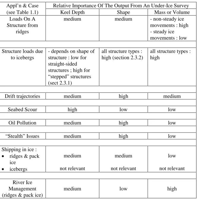
This section, and Table 2.4, provides comments regarding the relative importance of defining these parameters, in relation to the case(s) being considered.
Table 2.4 Information Requirements From Under-ice Surveys
Appl’n & Case Relative Importance Of The Output From An Under-Ice Survey (see Table 1.1) Keel Depth Shape Mass or Volume
Loads On A Structure from
ridges
medium medium - non-steady ice
movements : high - steady ice movements : low Structure loads due
to icebergs
- depends on shape of structure : low for straight-sided structures ; high for “stepped” structures (sect 2.3.1)
all structure types : high (section 2.3.2)
all structure types : high
Drift trajectories medium high medium
Seabed Scour high low low
Oil Pollution medium high low
“Stealth” Issues medium high low
Shipping in ice : • ridges & pack
ice • icebergs medium not relevant medium not relevant low not relevant River Ice Management (ridges & pack ice)
2.3.1 Parameter : Keel Depth
This is an important parameter for most cases (Table 2.4). However, the required accuracy, and extensiveness to which the keel depth needs to be defined, varies
significantly with the specific case being considered. Two of the cases that impose the greatest requirements (Table 2.4) are discussed below :
(a) interactions between ice features and subsea pipelines - it is well-known that the risk of damage to a buried pipeline, and the required burial depth, is very dependent on the keel depth distribution of the ice features contacting the seabed. An accurate knowledge of the keel depth distribution is required at the design stage. Keel draft information is also valuable for operational purposes (e.g., to guide ice management efforts as is being done at the Hibernia structure). (b) ice loads on an offshore structure with variable geometry - the loads on this type of structure (See Figure 2.7 for an example) are highly dependent on the depths of keels expected to be present near the structure. As a result, an accurate knowledge of keel depth is required to achieve an efficient design.
Figure 2.7
Iceberg Interaction With A Stepped Steel Gravity Platform (after Fitzpatrick and Kennedy, 1997)
2.3.2 Parameter : Ice Feature Shape
This parameter is most important for the following cases (Table 2.4) :
• loads on structures imposed by iceberg impacts - It is well-known that icebergs have a very variable geometry, and it is intuitively obvious that their shape plays a major role in controlling the forces generated during an impact. Iceberg shape is particularly important for structures with variable cross-section. Consider, for example, the interaction between an iceberg with “underwater rams” (e.g., Figure 2.8) with the stepped structure shown in Figure 2.7.
Unfortunately, little information is available in the literature to quantify the
significance of iceberg shape. Some inferences can be made from the work of Bass et al, 1985, who analyzed the loads resulting from eccentric, oblique collisions between a structure and an iceberg with three degrees of motion in the horizontal plane. They did not include the effect of motions in the vertical plane in their analyses. Bass et al, 1985, showed that the effect of variations in the vertical profile of the iceberg
depended on the obliqueness of the collision. For the range of values that they considered, they found that vertical profile variations could cause the maximum force developed during an impact to be reduced by up to about 50 %.
This value is supported generally by work done during the development of the Gravity Base Structure (GBS) for the Hibernia site which showed that the maximum load was reduced significantly when iceberg shape variations were included probabilistically in the load calculations (D. Nevel, Conoco, personal communication).
• iceberg drift trajectory predictions
• oil pollution analyses, and the available under-ice storage volume • “stealth” investigations
Figure 2.8
3.0 TECHNIQUES USED TO DATE FOR ENVIRONMENT DEFINITION STUDIES OF RIDGES AND HUMMOCK FIELDS
3.1 Overview
Figure 3.1 summarizes the techniques used to date for ice ridges and hummock fields. They can be broadly divided into two classes :
(a) bottom-mounted, upward-looking fixed installations, and ; (b) mobile systems
3.2 Bottom-Mounted, Upward-Looking Fixed Installations
These systems collect data at a specific location, and are best-suited for field
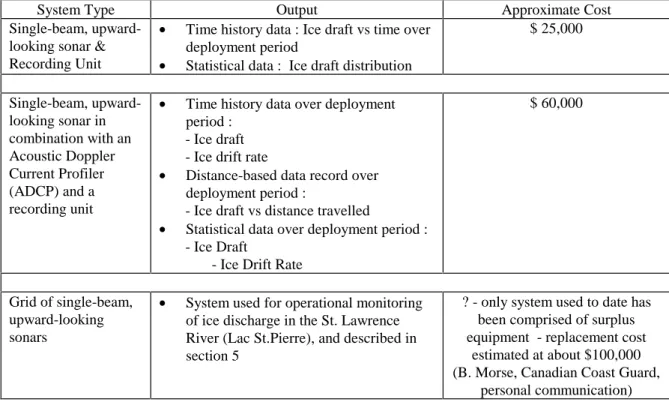
measurements in dynamic areas (where ice movements occur regularly) over long time periods. The types of bottom-mounted systems used to date are summarized in Table 3.1.
Table 3.1
Bottom-Mounted, Upward-Looking Fixed Installations
System Type Output Approximate Cost
Single-beam, upward-looking sonar & Recording Unit
• Time history data : Ice draft vs time over deployment period
• Statistical data : Ice draft distribution
$ 25,000 Single-beam, upward-looking sonar in combination with an Acoustic Doppler Current Profiler (ADCP) and a recording unit
• Time history data over deployment period :
- Ice draft - Ice drift rate
• Distance-based data record over deployment period :
- Ice draft vs distance travelled
• Statistical data over deployment period : - Ice Draft
- Ice Drift Rate
$ 60,000
Grid of single-beam, upward-looking sonars
• System used for operational monitoring of ice discharge in the St. Lawrence River (Lac St.Pierre), and described in section 5
? - only system used to date has been comprised of surplus equipment - replacement cost
estimated at about $100,000 (B. Morse, Canadian Coast Guard,
3.2.1 Single-Beam Upward-Looking Sonars With A Recording Unit
These are the simplest and cheapest systems, and they consist of a single transducer unit that continuously collects ice keel data as ice features pass over it. Most of the systems used to date for collecting ice keel data from fixed installations have been of this type. This type of system is presently being used at Confederation Bridge (which links Prince Edward Island and New Brunswick) to monitor ice conditions as part of an overall research program (M. Cheung, Dept of Public Works, personal communication).
Because these systems only collect keel draft data with respect to time, and not distance, they are only suited for the collection of statistical data and are unable to provide detailed keel profiles. Another disadvantage is that the data record can not be linked directly to the ice environment. For example, it is not known whether the data record is comprised of continuous “new” ice passing over the sensor, or of the same ice conditions being moved back and forth in the vicinity of the sensor.
This system type also has applications for operational monitoring. The New York Power Authority (NYPA) recently deployed such a system at the intake to its Niagara Falls power plant to warn of impending ice blockages. This system and deployment is described in section 5, (which discusses operational monitoring techniques). 3.2.2 A Combination Of An Upward-Looking Sonar And An Acoustic Doppler
Current Profiler (ADCP)
These systems provide significantly more information (than systems comprised of only single-beam sonars) because they measure both the ice drift rate and the ice keel draft as a function of time. This allows the ice keel draft record to be correlated against ice
movements and distance travelled.
They are a relatively recent development, having been developed and used over about the past five years.
3.2.3 Four Upward-Looking, Bottom-Mounted Sonars Deployed In A Grid Pattern The only system of this type used to date was deployed by the Canadian Coast Guard (CCG) to monitor ice discharge in Lac St. Pierre. With appropriate data processing, this system provided data regarding the ice drift rate, the ice thickness, and the ice discharge rate. This information was used to assist in making decisions regarding ice management in the St. Lawrence River (Morse et al, 1997), and it is described in section 5.
3.3 Mobile Systems : Overview
These systems are typically used to obtain profile or shape data for specific ice features that are actively selected by the user. Usually, in these applications, the field
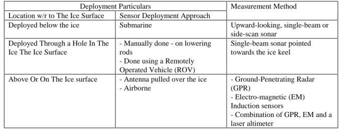
measurement efforts are aimed at documenting several ice features in a region of interest (e.g., to establish a database) in a relatively short time. The platforms and approaches used for mobile systems are summarized in Figure 3.1, and they fall into the general classes listed in Table 3.2.
Table 3.2 Mobile Systems : Deployment Surface & Measurement Methods
Deployment Particulars Measurement Method Location w/r to The Ice Surface Sensor Deployment Approach
Deployed below the ice Submarine Upward-looking, single-beam or side-scan sonar
Deployed Through a Hole In The Ice The Ice Surface
- Manually done - on lowering rods
- Done using a Remotely Operated Vehicle (ROV)
Single-beam sonar pointed towards the ice keel
Above Or On The Ice surface - Antenna pulled over the ice - Airborne - Ground-Penetrating Radar (GPR) - Electro-magnetic (EM) Induction sensors - Combination of GPR, EM and a laser altimeter
3.4 Mobile Systems Deployed From Below The Ice Surface
Submarines have been used to a limited extent to obtain statistical data regarding ridge keels (e.g., Wadhams and Horne, 1980). The primary advantage of this approach is that a large quantity of data can be collected along various tracks in a short time.
The disadvantages of this approach are that :
(a) it is difficult, if not impossible, to obtain data regarding the sail portion of the ice track for correlation.
(b) submarines are an expensive logistical platform (c) submarines are not readily available
(d) usually, the survey track position, and time of survey, can only be provided to low precision (because this information is classified). The location can usually only be obtained to tenths of degrees of latitude and latitude, and the time of survey to within a few weeks.
3.5 Mobile Systems Deployed Through A Hole In The Ice Sheet
Two general types of systems have been used to obtain profile data by deploying sonars through the ice as follows :
(a) sonar transducers mounted on lowering rods that are deployed from the ice surface ; and
(b) sonar transducers mounted on Remotely Operated Vehicles (ROVs). 3.5.1 Manual Deployments Using Lowering Rods
Many projects have been conducted using this approach, some of which are referred to in Figure 3.1. This method is relatively inexpensive, as the logistical requirements are minimized. This approach also has the advantage that the sails and keels of the ice feature can be accurately linked to each other using standard surveying techniques. Of course, this method requires that the ice surface be stable, and thus that it provides a safe working platform.
The earliest profiling projects carried out from the ice surface were conducted by mounting the sonar transducer on rods such that the sonar ranged horizontally. To measure the keel profile, the sonar transducer was lowered below the ice surface by adding more rods to the string which allowed range data to be collected at each step (Figure 3.2a).
One major disadvantage with this approach was that a great deal of scattering occurred as this arrangement causes the sonar beam to contact the ridge keel at unfavourable angles. This arrangement was improved significantly during a project conducted by NORCOR, 1976 (to profile multi-year ridge keels) by building a rotating-arm apparatus at the lowest lowering rod (Figure 3.2b). This allowed the sonar head to be rotated through 90° which provided for much more favourable contact angles and for significantly stronger sonar returns.
In recognition of the importance of limiting backscattering, most ice ridge keel survey projects conducted since the early 1980’s (e.g., Geisel et al , 1982) have been undertaken using scanning sonar systems (Figure 3.2c).
Figure 3.2
Sonar Deployments From The Ice Surface
(a) Sonar Mounted On Lowering Rods And Ranged Horizontally
(b) Hinged Lowering Rod Approach
3.5.2 Deployments Using Remotely Operated Vehicles (ROVs)
A small number of projects have been conducted using ROVs to support sonars for measuring the keels of ice ridges and hummock fields. The earliest efforts (to our knowledge) were conducted by Harrington and St. John, 1987. These efforts were relatively unsuccessful as the ice drafts measured using the ROV did not correlate well with the measurements made by direct drilling. Harrington and St. John, 1987 attributed this to positioning errors for the ROV.
More recently, surveys were undertaken by the Institute of Ocean Sciences (IOS) using an improved ROV to map the under-ice surface of a hummock field and a ridge in the
Beaufort Sea (Melling et al, 1993 ; and Bowen and Topham, 1996, respectively). These surveys were successful in that a 3-D map of the under-ice surface was produced. The ROV used during Melling et al, 1993’s ; and Bowen and Topham, 1996’s surveys was a “Tethered Arctic Reconnaissance Submersible” (TARS) manufactured by
International Submarine Engineering Ltd. of Port Moody, BC. Under-ice surveys were accomplished by driving the TARS out under power along a series of radial lines from an access hole in the ice to a maximum range of about 150 m. When the TARS reached the end of its tether, it was hauled back manually to the deployment hole. This survey length (of 150 m) was considered to be close to the maximum that can be used effectively with the TARS as at large tether lengths, the drag on the umbilical tended to “fly the ROV” (H. Melling, IOS, personal communication). The TARS was deployed to the site(s) using Twin Otter aircraft.
The TARS was fitted with an upward-looking sonar that gave a nominal resolution of 12 cm at a range of 30 m, and a positioning system that had a nominal positional accuracy of +/- 20 cm. Bowen and Topham, 1996, reported that tests against a known position “suggested that accuracies of this order were realised in operation”.
3.5.3 Deployments Using Autonomous Underwater Vehicles (AUVs)
To our knowledge, no deployments have been made to date using AUVs to obtain under-ice profile data. However, this would be within the capabilities of present-day AUVs, with some modifications, as demonstrated by the Theseus’s recent success in laying fibre-optic cables in the Arctic (Thorleifson et al, 1997).
3.6 Mobile Systems Deployed From Above Or On The Ice Surface Two types of systems fall into this category, as follows :
(a) Ground-Penetrating Radars (GPR)
(b) Electro-Magnetic (EM) Induction systems
3.6.1 Ground-Penetrating Radars
Past deployments have been carried out using both airborne systems (e.g., Paulley and Gehrig, 1987 ; O’Neill and Arcone, 1991) and sled-mounted systems that were pulled over the ice (e.g., Kovacs and Morey, 1989).
Both freshwater and saline ice sheets have been successfully profiled (Arcone, 1985 ; Kovacs and Morey, 1989). In addition, multiyear ice ridges have been successfully profiled (e.g., Paulley and Gehrig, 1987).
It is well-known that GPRs are most suitable for profiling “simple” ice conditions (such as sheet ice and/or relatively small multi-year ridges) in which the ice is relatively
uniform (with respect to its dielectric properties). It is also well-known that this technique suffers from inaccuracies for “complex” ice conditions, such as first year ridges and brash, where the dielectric properties of the ice are non-uniform, as the internal reflections caused by these features introduces scattering and distortion of the signal. During trials with an airborne system over Arctic sea ice, Paulley and Gehrig, 1987 found that the measured ice thicknesses agreed with the ground truth values within 10 % for ice thicknesses up to 9 m (30 ft). However, trials over brash ice were relatively unsuccessful (Arcone et al, 1986) as the brash ice distorted signals and allowed no discernible bottom return.
3.6.2 Electro-Magnetic (EM) Induction systems
Most deployments with EM systems have been airborne although a small number of test programs have been conducted by means of handheld deployments.
The development of EM systems has progressed from an experimental to a “semi-operational” status with the result that its capabilities are relatively well-known. EM systems are suitable for measuring the thickness of ice features in seawater, whereas they are incapable of operating for ice features in freshwater.
Most recently, the “Ice Probe” has been built and used on a near-operational basis. The “Ice Probe” employs an EM system, along with a snow thickness ground-penetrating radar, and a laser altimeter, and is described in detail in section 5.3.
4.0 TECHNIQUES USED TO DATE FOR ENVIRONMENT DEFINITION STUDIES OF ICEBERGS
4.1 General
Iceberg surveys have been done to measure draft, mass and shape. The profiling
techniques used to date fall into the two general classes below, and they are summarized in Tables 4.1 and 4.2.
(a) above-water techniques - these include observations of the iceberg’s sail using photography, radar or other surveying techniques ; and ground-penetrating radar. (b) below-water techniques using sonars.
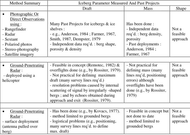
Table 4.1 Summary Of Above-Water Profiling Techniques Used To Date For Icebergs
Method Summary Iceberg Parameter Measured And Past Projects
Draft Mass Shape
• Photographic Or Direct Observations using : - Rangefinder - Radar - Sextant - Polariod photos - Stereo-photography - Satellite imagery
Many Past Projects for icebergs & ice shelves :
- e.g., Anderson, 1984 ; Farmer, 1967, Smith, 1987, Dempster, 1979
- Independent data req’d. : berg shape, porosity & density
Has been done : - Independent data req’d. : berg density, porosity - Past deployments : Anderson, 1984 ; Farmer, 1967 Not a feasible approach • Ground-Penetrating Radar : - deployed using a helicopter
- Feasible in concept (Remotec, 1982) & overflights done (e.g., by Rossiter, 1979). - Not practical for defining maximum draft (many survey lines req’d.)
- resolution problems caused by internal scattering of signal by irregularly -shaped bergs ; and by echoes obtained during approach and exit (Rossiter, 1979).
- Not practical for defining mass (many lines req’d, positioning errors) although overflights have been done (e.g., by Rossiter, 1979) Not a feasible approach • Ground-Penetrating Radar : - surface deployment (antenna pulled over berg)
- Has been done (e.g., by Kovacs, 1977). - method limited to grounded bergs - logistical problems (e.g., positioning, many survey lines req’d. to define max. draft)
- Feasible in concept but not done to date
- method limited to grounded bergs
Not a feasible approach
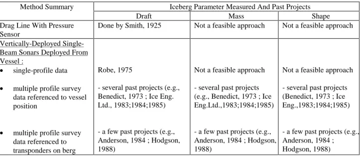
Table 4.2 Summary Of Below-Water Profiling Techniques Used To Date For Icebergs
Method Summary Iceberg Parameter Measured And Past Projects
Draft Mass Shape
Drag Line With Pressure Sensor
Done by Smith, 1925 Not a feasible approach Not a feasible approach Vertically-Deployed
Single-Beam Sonars Deployed From Vessel :
• single-profile data
• multiple profile survey data referenced to vessel position
• multiple profile survey data referenced to transponders on berg
Robe, 1975
- several past projects (e.g., Benedict, 1973 ; Ice Eng. Ltd., 1983;1984;1985)
- a few past projects (e.g., Anderson, 1984 ; Hodgson, 1988)
Not a feasible approach - several past projects (e.g., Benedict, 1973 ; Ice Eng.Ltd.,1983;1984;1985)
- a few past projects (e.g., Anderson, 1984 ; Hodgson, 1988)
Not a feasible approach - several past projects (Benedict, 1973 ; Ice Eng.,1983;1984;1985)
- a few past projects (e.g., Anderson, 1984 ;
Hodgson, 1988)
4.2 Above-Water Techniques
The above-water techniques fall into two general categories as described below : (a) Iceberg Sail Observations - Several techniques using photography or direct observations have been used to quantify the iceberg sail (Table 4.1). Attempts have been made to infer iceberg draft and/or mass using these data and other independent information and relationships (e.g., berg density, berg shape, relationships with berg length or plan area, etc.).
It is generally recognized that these techniques are only capable of providing first order information. The only parameter that can be defined to reasonable accuracy using this technique is the iceberg mass. For relatively high-precision surveys conducted using aerial stereo-photography for the icebergs profiled during the DIGS (Dynamic Iceberg Grounding Study) project, Hodgson et al, 1988 estimated that the calculated above-water volumes were accurate to within approximately +/- 2 %. However, because the iceberg sail represents only about 10 % of the iceberg’s total volume, this inaccuracy (of +/- 2 %) represents an inaccuracy in total iceberg volume of about +/- 20 %.
The use of iceberg sail observations for inferring draft information is more problematic because icebergs have a very wide range of shapes, which are difficult to categorize. Many past projects have been conducted to infer iceberg draft from various sail measurements and/or shape classifications. In general, these studies have shown that iceberg draft can only be estimated approximately from sail observations.
Iceberg sail observations are incapable of providing information regarding iceberg shape.
(b) Iceberg Keel Measurements Using Surface Or Aerial Observations Made With Ground-Penetrating Radar - Grounded icebergs have been profiled by pulling the antenna over the iceberg (Kovacs, 1977). Floating icebergs have been profiled using ground-penetrating radar deployed by helicopter (e.g., by Rossiter, 1979). For grounded icebergs, this technique is capable of defining iceberg mass
relatively well, in combination with other survey data. The maximum draft could also be determined although extensive surveys would be required. This technique is not considered capable of providing iceberg shape data.
For floating icebergs, ground-penetrating radar must be deployed by helicopter which makes it infeasible to obtain the maximum draft (Table 4.1), and most likely the iceberg mass. However, this technique allows a large number of icebergs to be profiled quickly, and consequently, it is considered to be most suited for the collection of statistical data.
The reader is cautioned that past deployments have shown that this technique (of using aerially-deployed GPRs) suffers from resolution problems caused by internal scattering and reverberations of the signal (e.g., Rossiter, 1979).
4.3 Below-Water Techniques
Most programs to survey icebergs using under-water techniques have been conducted by deploying sonars in the water. The methods differ with respect to :
(a) the objectives of the surveys ; and
(b) the methods used for referencing the position of the sonar during iceberg surveys conducted from a support vessel
4.3.1 Iceberg Draft Surveys
The earliest measurements of iceberg draft were made by Smith, 1925, who pulled a towline, with a pressure sensor mounted on it, under an iceberg.
Figure 4.1
Most recently, the drafts of icebergs approaching the subsea line between the Gravity Base Structure (GBS) and the offshore Loading System (OLS) at Hibernia will be monitored. The techniques for this operational monitoring program are discussed in section 5.
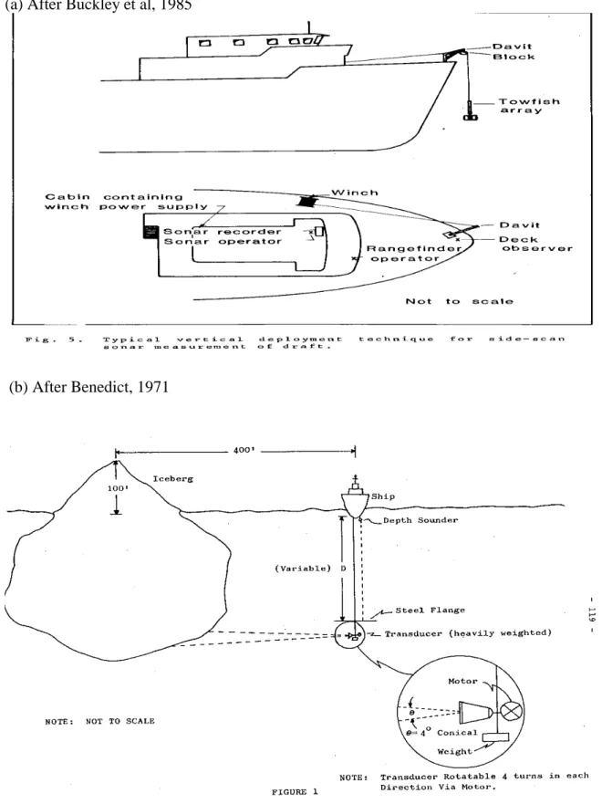
4.3.2 Surveys Aimed At Measuring Iceberg Shape, Mass, And Draft
These surveys have been carried out by deploying a sonar vertically from a support vessel.
Early surveys (e.g., Benedict, 1973 ; Ice Eng. Ltd., 1983; 1984; 1985) were conducted by referencing the sonar to the vessel, and to the berg (Figure 4.2). Buckley et al, 1985, observed that this method produces large errors as a result of a number of sources, including :
(a) transducer attitude error ; (b) transducer positional error ; (c) azimuth ambiguity ;
(d) vertical ambiguity ; and (e) detection problems caused by :
(i) increasing range to the iceberg at large keel depth ; and
(ii) little to no sonar return from the iceberg caused by contact of the sonar beam with the iceberg at unfavorable angles.
Figure 4.2 System Used To Measure Iceberg Shape And Draft : Sonar Transducer Position Referenced to The Survey Vessel (a) After Buckley et al, 1985
Buckley et al, 1985, concluded that this method provides only a “rough” measurement of ice draft, with “confidence limits of accuracy that are at best 10 to 15 %”. They also concluded that it was “inadequate for the determination of the underwater shape”. Recognizing these limitations, a more accurate system was devised by H.Lanzanier, in which the sonar was independently referenced to transponders placed on the berg (Figure 4.3). This system was used in surveys by Anderson, 1984, and Hodgson, 1988.
Figure 4.3
System Used To Measure Iceberg Shape And Draft : Sonar Transducer Position Referenced To Transponders On The Iceberg (after Hodgson et al, 1988)
With this method, surveys were conducted using the following general approach : (a) a polypropylene rope with 4 or more transponders attached to it was strung around the iceberg at the waterline using a support vessel.
(c) After the iceberg had been profiled along one face, the survey vessel was moved around the berg to another location and that face of the berg was profiled. (d) the full data set were then reduced, and synthesized to produce a three-dimensional shape of the iceberg.
This system resolved many of the inaccuracies associated with the earlier systems. The positional accuracy of the sonar transducer was improved to an expected value of about 1 m (H. Lanzanier, personal communication). Furthermore, because there was overlap between individual survey points, post-processing routines could be used to check for and to minimize errors. Attempts were also made to minimize errors using post-processing routines based on hydro-statics and iceberg stability.
Although the overall accuracy of the approach was improved, considerable errors were still present as significant post-processing was required to ensure that hydro-static and stability criteria were met (J. Lever, CRREL, personal communication). Hodgson et al, 1988 estimated that the under-water volumes calculated for the icebergs profiled during the DIGS project were accurate to within approximately +/- 15 %.
As well, this system had some other limitations, as follows :
(a) safety - it was necessary for the survey vessel to be in close proximity to the iceberg in order to deploy the rope around the iceberg at its waterline.
Safety hazards were also present during the sonar data collection part of the operation. Although lower-frequency sonars were used to increase their range, and thus increase the vessel “standoff distance” (H. Lanzanier, personal
communication), it was still necessary to position the vessel relatively close to the iceberg (i.e., within about 200 m), which causes potential safety hazards. For example, it was later discovered that during the DIGS project, the survey vessel had been positioned at times over “underwater rams” (see Figure 2.8 for example) of the berg (J. Lever, CRREL, personal communication).
(b) the time required to conduct surveys - About 0.5 to 1 day was required to survey an iceberg using this method which was considered to be rather long (J.Lever, CRREL, personal communication). This imposed relatively high data collection costs, as it required a relatively large amount of ship time while limiting the number of icebergs that can be surveyed. Furthermore, this long time period introduced other difficulties as conditions could change over the duration of the survey. For example, the icebergs sometimes rolled during the course of the survey, resulting in incomplete data (H. Lanzanier, personal communication). (c) support platform requirements and limitations
5.0 TECHNIQUES USED TO DATE FOR OPERATIONAL MONITORING The literature search conducted in this project revealed only a few cases where under-ice data have been collected as part of an operational monitoring program, as summarized in Table 5.1. Further information is provided in the following sections.
Table 5.1
Operational Monitoring Applications and Systems Used
Application General Description Of System Approximate Cost Ice discharge monitoring
in the St. Lawrence River by the Canadian Coast Guard (CCG)
Four upward-looking single-beam sonars deployed in a grid pattern, in combination with data acquisition hardware, a sonar controller, and data processing software
? Surplus equipment used -replacement cost estimated at about $100,000 (B. Morse, CCG, personal communication)
Ice thickness monitoring near the New York Power Authority’s (NYPA) water intakes for the Niagara Power Project
Dual-frequency, single-beam upward-looking sonar in combination with data acquisition hardware, a sonar controller, and data processing software
$ 25,000
Ice surveys conducted in the Gulf of St. Lawrence to assist routing
recommendations for icebreakers and shipping
The “Ice Probe” - an airborne system deployed using a helicopter that consists of an electro-magnetic induction sensor, a snow thickness ground-penetrating radar, and a laser altimeter
? - system has been developmental to date - replacement cost estimated at about $250,000 (S. Halliday, Aerodat Inc., personal communication) Iceberg Draft Monitoring
for icebergs approaching the subsea pipeline between the GBS and the OLS at Hibernia
Three supply vessels are outfitted with scanning sonars. The vessel(s) approaches bergs of concern, and surveys their draft.
? - two of the vesels were already outfitted with hull-mounted sonars. The third one is outfitted with a 360° scanning sonar deployed using a stern winch. The cost of the scanning sonar is about $ 50,000.
5.1 Application : Monitoring Of Ice Discharge In The St. Lawrence River 5.1.1 Past Deployments
The objectives of this deployment were to obtain ice thickness and drift rate data (Morse et al, 1997). These results were inputs for determinations of the ice discharge, which was used for guiding ice management efforts, such as the deployment of icebreakers. Two general systems were tried as follows :
“pushed aside” by ice, and thus to be unreliable (B. Morse, Canadian Coast Guard, personal communication). After making some design changes, CCG intends to redeploy this system this coming winter.
It should be noted that the system was redesigned to fit inside a drum and
redeployed during March, 1998, with more success. The data are currently being analyzed. The reader should contact the CCG for further information
The acoustic system (i.e., item (a) above) consisted of four 200 kHz upward-looking sonars, in combination with a controller and a PC computer. The transducers were spaced 2.44 m apart and mounted on the four corners of a steel frame that was located in the shipping channel of Lac St. Pierre. The frame was levelled upon installation.
However, its attitude was not measured during the deployment. Post-processing software was developed to allow the ice thickness and the ice drift rate to be determined. These parameters were used to estimate the ice discharge, in combination with observations of the shipping channel width.
The ice conditions ranged from sheet ice to rubbled, ridged and rafted pack ice. Most of the ice thicknesses measured were below 1.5 m, although some cases up to about 3.5 m (which most probably consisted of rubbled ice pack) were recorded.
The ice thickness was determined based on a knowledge of the range to the air/water interface, and the range to the under-ice surface. Morse et al, 1997 reported that the water level and the ice thickness estimates were within 1 to 2 cm, and 5 cm, respectively, based on comparisons among the four transducers.
The ice drift rate was determined based on the time interval at which individual ice features appeared on the sonar records. Morse et al, 1997, reported that the speeds determined from individual pairs of transducers agreed with each other within 5 cm/s, “when the ice features are well-defined and the data is relatively clean”.
Morse et al, 1997 reported that the system provided excellent data capture which they attributed to redundancy, real-time access and near real-time data treatment, and fully-armoured protective hoses for data transmission.
5.1.2 Future Developments
The Canadian Coast Guard plans to deploy a second system this coming winter (B. Morse, Canadian Coast Guard, personal communication). This system will be comprised of an Acoustic Doppler Current Profiler (ADCP). One unique feature of the planned deployment for this winter is that data transmission by magneto-induction from the riverbed to a nearby shore-based receiver will be tried. This is an emerging technology that avoids the requirement for direct cabling. It is described further in Annex A.
5.2 Application : Monitoring Of Ice Conditions At The Niagara Power Project’s Water Intakes
The objective of this field demonstration was to measure the ice thickness in the Upper Niagara River in the vicinity of the New York Power Authority’s (NYPA) water intakes for the Niagara Power Project. Previous studies (e.g., Shen and Su, 1996) have shown that this information would assist decision-making regarding ice management operations. The deployed system (described in Canpolar, 1997) consisted of a dual-frequency
upward-looking sonar, with operating frequencies of 50 and 200 kHz, an inclinometer, a controller, and a personal computer. Post-processing software was developed to : (a) filter the data to remove noise ; and (b) calculate the ice thickness based on sequential measurements of the range to the air/water interface, and the under-ice surface. The field demonstration was conducted over the 1994-95 winter season.
The water levels measured with the sonar system were consistently within about 10 cm of those measured at the NYPA’s intake water level. Canpolar, 1997 stated that this implies that the depth of the ice below the water surface can be measured with the sonar to within about 10 cm. Canpolar, 1997, found that the low-frequency sonar (which operated at 50 kHz) provided the most reliable measurements of the range to the ice-water interface. They suggested that a single-frequency transducer would be adequate for an operational system.
Canpolar, 1997 concluded that the system was demonstrated to be feasible for its intended purpose. However, they cautioned that the system needed to be tested over a wider range of conditions before general statements could be made. They also cautioned that further developments (with respect to the analysis software and the diagnosis of electrical noise problems) were necessary before the system could be used operationally. 5.3 Application : Route Selection For Icebreakers And Ships Operating In Ice In The
Gulf of St. Lawrence
Airborne ice thickness surveys were carried out at some times by the Canadian Coast Guard (CCG) during the 1996-97 winter as part of the process of making routing
recommendations for ship and icebreaker captains operating in the Gulf of St. Lawrence. It is hoped that eventually these surveys will become part of their routine operations. However, to date, they have been done on a trial basis (A. Maillet, CCG, personal communication).
Prinsenberg et al, 1991 ; Topham and Bowen, 1996) ; the Labrador Sea (Holladay et al, 1992) ; and the east coast of Newfoundland (Holladay and Rossiter, 1990).
The Ice Probe survey results were primarily used to help ground-truth and/or confirm visual observations of different sheet ice types (e.g., young ice, gray ice, gray-white ice, first year ice, etc.) that were identified from helicopter ice reconnaissance missions or from satellite imagery analyses. The ice thickness data obtained from the Ice Probe provided useful complementary data to, and verification of, the visual observations (A. Maillet, CCG, personal communication). The snow thicknesses measured by the Ice Probe Surveys were also of value for defining route conditions.
The system was found to provide an accurate and useful measurement of the level ice thickness, which is generally similar to the results obtained during Arctic trials. Prinsenberg et al, 1992, found that the Ice Probe measured the sheet ice thickness to within about +/- 5 %, or 0.1 m.
The Ice Probe was also used to provide ice thickness data for deformed ice (e.g., ridges, rafted ice, pack ice) although the thicknesses of these ice types was significantly
underestimated (by about 50 %). These results are similar to those from field trials in the Arctic (Prinsenberg et al, 1992). Topham and Bowen, 1996, attributed this to : (a) the large footprint of the Ice Probe, which is of the order of the Ice Probe’s altitude (typically about 30-60m) ; and (b) the porous nature of first-year ridges which results in a large bulk electrical conductivity, thus producing a poorly defined interface. Nevertheless, because ships tend to “average” out ice conditions when transitting a ridged ice field, these “average” thicknesses indicated by the Ice Probe were considered to be valuable information.
It is hoped that that eventually this system will become an operational tool (A. Maillet, CCG, personal communication), and the CCG intends to continue them in the upcoming winter. However, at present, it is an emerging technology, and as a result, a number of problems were encountered. For example, the Ice Probe crashed during the 1996-97 winter (as a result of an engine failure by the helicopter), which caused a long downtime period.
5.4 Application : Iceberg Draft At The Hibernia Structure
The objective of this program is to monitor the drafts of icebergs that approach the subsea line between the Gravity Base Structure (GBS) and the Offshore Loading System (OLS). This information will be used to help determine whether or not ice management efforts should be undertaken (L. Davidson, Agra Ltd., personal communication). Three supply vessels, each one equipped with a 675 kHZ scanning sonar, will be used in the program which will be conducted by : (a) approaching icebergs of interest ; (b) deploying the sonar (for one of the vessels - the other two have hull-mounted sonars) ; and (c) measuring the iceberg’s draft.
6.0 THE PRESENT STATE-OF-THE-ART AND RECOMMENDATIONS 6.1 Ice Features Of Interest : Ridges And Hummock Fields
The general cases of interest for these ice features are summarized in Table 6.1. Table 6.1
Profiling Ridges And Hummock Fields : General Cases Of Interest
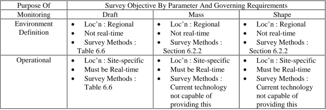
Purpose Of Monitoring Survey Objective By Parameter & Governing Requirements
Program Keel Draft Keel Shape And/or Volume
Environment Definition • Loc’n : Site-specific or regional
• Timeliness : Not real-time
• Survey Methods : Table 6.2
• Loc’n : Site-specific or regional
• Timeliness : Not real-time
• Survey Methods : Table 6.3 Operational • Location : Site-specific
• Timeliness : Must be Real-time
• Survey Methods : Table 6.4
• Location : Site-specific
• Timeliness : Must be real-time
• Survey Methods : Current
technology not suited to provide this
6.1.1 Survey Objective : Environment Definition
The recommended methods for monitoring keel draft are summarized in Table 6.2 and depend upon :
(a) the location or area of interest (e.g., regional vs site-specific) - Bottom-mounted systems are preferable for site-specific surveys. For regional surveys, two general approaches are possible :
(i) deploy several bottom-mounted systems, and/or ;
(ii) use a mobile system, such as an Autonomous Underwater Vehicle (AUV) or submarine.
The use of several bottom-mounted systems has the advantage that ice keel flux rates across given boundaries can be determined. Mobile systems are better-suited to collecting statistical data as a larger quantity of data can be obtained in a shorter time period.
(b) whether or not the ice cover is highly mobile - This has the greatest effect on the feasibility of using bottom-mounted systems. Clearly, bottom-mounted systems are not feasible for sites where ice movements are small.
Table 6.2
Profiling Methods For Environment Definition Surveys : Draft Of Ridge Keels And Hummock Fields
Survey Ice Cover Available Approach And Systems
Area Mobility Method Survey Output Sensor Cost
Site-Specific
High Bottom-Mounted : Single-beam, upward-looking sonar & Recording Unit
• Time history data : Ice draft vs time over deployment period
• Statistical data : Ice draft distribution $ 25,000 High Bottom-Mounted : Single-beam, upward-looking sonar in combination with an Acoustic Doppler Current Profiler (ADCP) and a recording unit
• Time history data over deployment period :
- Ice draft - Ice drift rate
• Distance-based data record over deployment period :
- Ice draft vs dist. travelled
• Statistical data over deployment period :
- Ice Draft
- Ice Drift Rate
$ 60,000
Site-Specific
Low Not a relevant case
Regional Not Important
Deploy several of the above Bottom-Mounted Systems
• As above for the systems selected
• Keel flux rate across boundaries
- depends on no. of systems Not Important Mobile Systems : • Autonomous Underwater Vehicle (AUV) • Submarine
• Keel draft distribution along survey lines AUV : $1,500,000 Submarine : ? (See notes) Notes :
1. AUV Costs - Because AUVs are not generally available for lease (as our equipment survey only found one case where AUVs might be leased), the approximate purchase cost of a AUV that would be capable of conducting this type of survey is listed here.