HAL Id: halshs-02794605
https://halshs.archives-ouvertes.fr/halshs-02794605
Preprint submitted on 5 Jun 2020
HAL is a multi-disciplinary open access
archive for the deposit and dissemination of sci-entific research documents, whether they are pub-lished or not. The documents may come from teaching and research institutions in France or abroad, or from public or private research centers.
L’archive ouverte pluridisciplinaire HAL, est destinée au dépôt et à la diffusion de documents scientifiques de niveau recherche, publiés ou non, émanant des établissements d’enseignement et de recherche français ou étrangers, des laboratoires publics ou privés.
Extreme and Persistent Inequality: New Evidence for
Brazil Combining National Accounts, Surveys and Fiscal
Data, 2001-2015
Marc Morgan
To cite this version:
Marc Morgan. Extreme and Persistent Inequality: New Evidence for Brazil Combining National Accounts, Surveys and Fiscal Data, 2001-2015. 2017. �halshs-02794605�
World Inequality Lab Working papers n°2017/12
"Extreme and Persistent Inequality: New Evidence for Brazil Combining
National Accounts, Surveys and Fiscal Data, 2001-2015"
Marc Morgan
Keywords : Income Inequality; top incomes; distribution; Brazil; DINA;
Distributional National Accounts; inequality; capital;
Falling Inequality beneath Extreme and Persistent Concentration:
New Evidence for Brazil Combining National Accounts, Surveys and
Fiscal Data, 2001-2015
Marc Morgan* First draft: 10 August 2017 Online publication: 1 September 2017 This version: 22 February 2018 Abstract This paper re-examines the evolution of income inequality in Brazil over the last fifteen years using a novel combination of data sources. We measure distributional national accounts (DINA) to produce a new series of pre-tax national income inequality, combining annual and nationally representative household survey data with detailed information on income tax declarations, in a consistent manner with macroeconomic totals. Our results provide a sharp upward revision of the official estimates of inequality in Brazil, while the falling inequality trends are less pronounced than previously measured. The concentration of income at the top is striking, with the Top 1% income share increasing to 28.3% by the end of the period, from an initial share of 26.2%. The Top 10% increased their share of income from 54.3% to 55.6% of pre-tax national income and captured 62.5% of total growth. The Bottom 50% share rose from 12.6% to 13.9%, experiencing higher growth than the top decile, but capturing only 20% of total growth due to its extremely low command of income. While elites and the poor made gains, the Middle 40% of the distribution decreased its share from 33.1% to 30.6%, posting less growth than the average for the whole economy. The “squeezed middle” is a product of its relatively low share of income and poor growth performance. Overall, inequality within the bottom 90% declined while concentration at the top grew, effects manifested in the slight downward trend of the corrected Gini coefficient. The former was driven by falling inequality in the distribution of labour income, which we document after combining surveys and fiscal data. While labour income inequality (and especially the formal earnings component) registered a clear decline according to our series – following the sharp rise in the real minimum wage, falling informality and fading out of the education premium – it was insufficient to mitigate the extreme inequality of capital resources and reverse the growing concentration of national income among elite groups.* Paris School of Economics & World Inequality Lab, 48 Boulevard Jourdan, 75014 Paris (e-mail:
marc.morgan@psemail.eu). For their helpful comments I thank Thomas Piketty, Facundo Alvaredo, Lucas Chancel, Ignacio Flores, Mauricio de Rosa, Rodrigo Orair and other seminar participants at IPEA and IPC-IG in Brasilia, and at the First WID.world Conference in Paris. I gratefully acknowledge funding from the Fundación
1. Introduction From a region historically characterized by high and persistent levels of income inequality – since at least the late 19th century (Williamson, 2015) – Brazil is no exception to being under the spotlight in this domain. In any official report on income distribution by an international organization, Brazil usually features near the summit of the inequality rankings, as measured by household survey data, alongside some of its regional counterparts such as Colombia, and South Africa. While most studies on income inequality in developing countries use either survey-based measures or tax-based measures of inequality (when available), this paper combines national accounts with nationally representative household survey data (from the national statistics office) with detailed tabulations on income tax declarations (recently released by the federal tax office) in a consistent manner to produce two new series of inequality for Brazil – a series of pre-tax fiscal income inequality and a series of national income inequality across the entire distribution. We thus construct a set of distributional national accounts (DINA) for Brazil. We compare these series with the series estimated from the raw survey data (prior to any correction) and with a new corrected series of labour income inequality, where we combine the same data sources to distribute labour incomes.
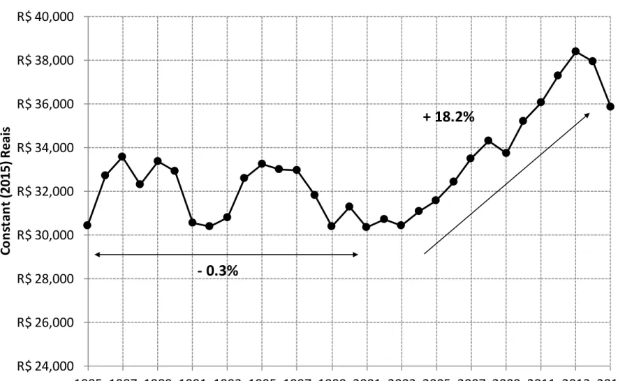
The fifteen years since the turn of the new century in Brazil are an interesting period to study because it marks the return of economic growth after the prior fifteen years of
stagnation (see Figure 1). Average adult incomes expanded by 18% in the world’s 8th largest
economy and 3rd largest parliamentary democracy. Politically, it is also an interesting period due to the coming to power of the first “Labour Party” government in Brazil since the early 1960s, with the election of Lula da Silva to the presidency and his Worker’s Party (PT) compatriots into congress in late 2002. New innovations were brought about in the field of social policy to tackle poverty, such as the Bolsa Familia conditional cash transfer program, and a higher share of fiscal receipts were dedicated to social spending as the share of total government spending in the economy rose over the period. The PT government also brought about negotiations that increased the real value of the minimum wage considerably during their mandate. These are variables that are strictly tied to the distribution of income. And as such, their effects should be traceable in the statistics on inequality. This line of thinking built the consensus that identified a significant decline in income inequality in Brazil, as
elsewhere in Latin America, at least according to official measures relying on household surveys (see López-Calva and Lustig, 2010 and Lustig et al. 2016).
A number of reasons motivate why we combine fiscal data and survey data to measure the distribution of income. The most obvious one is almost exclusive reliance on household self-reported surveys to assess income distributions in Brazil. While the true income distribution is unobserved, household surveys can approximate a personal income distribution by expanding the frequencies of a representative sample of the population. The problem with surveys is that they tend not to include complete information on the very rich in the studied country. Despite random sampling, their income is either not well measured or are not observed, due to the reluctance of the richest individuals to disclose all of their income sources, particularly their assets. Additionally, the rich may refuse to engage in the time-consuming task of answering a comprehensive household survey, assuming that interviewers manage to enter the gated communities in which they live. Moreover, statisticians may intentionally remove extreme observations, so as to top-code the distribution. Surveys are thus prone to over-represent the extent of labour income at the top of the distribution and underestimate the extent of capital income distributed to households compared to what the national accounts would imply. Income tax data, on the other hand, better captures richer individuals, as filing a declaration is obligatory above specified income thresholds, and in many cases, there is third party reporting. Although not everybody declares income to the fiscal authorities and some people can be tempted to under-declare their income in order to pay less tax, we can be quite confident in thinking that the people appearing in tax data actually exist (as they are well identified by fiscal procedures) and earn at least what they declare. This paper is thus among the first to use personal income tax records to study distributive issues, but it is not the only one. Medeiros et al. (2015) and Gobetti & Orair (2016) have also contributed to show that tax data convey a different picture of Brazilian inequality than that which was previously released using surveys. However, our study is the first to generate a series of distributional national accounts (DINA). This is important for two main reasons. First, by being anchored to the national accounts, DINA allow us to distribute the proceeds of growth as measured and diffused by official sources. This was not possible in previous
studies because the income concept used had less of a direct relation with macroeconomic growth. Second, and more importantly, DINA allow us to see to whom in the hierarchy income originally flows. While it may be argued that fiscal income (i.e. income received by households that is subject to assessment by the tax authorities) or disposable income (i.e. income individuals actually dispose of after government taxes and transfers) are more relevant, the distribution of national income gives us insights into the distribution of economic resources, including corporations, pension funds, insurance funds and real estate. It is thus more intricately connected with the distribution of capital and power. This can often be more crucial than the distribution of disposable income as it precedes it in the flow of funds and can thus determine the society’s capacity for redistribution.
Our focus on pre-tax inequality is in contrast to most studies that concentrate on disposable (i.e. net) income inequality. While this focus is necessary to assess the role of the state in the redistribution of income in Brazil, its sole use detracts from the market distribution of income in the country, which can be seen as the precursor to the secondary (disposable) distribution of income. Therefore, by dealing with the original distribution of income under the DINA framework, this paper provides a different angle from which to analyse income inequality in Brazil. But we also consider the impact that Brazil’s celebrated cash transfer programs have on the distribution of income, factoring them into the estimates using a simple and transparent method.
We present our main results in the form of income shares because they help to stratify the income-generating population into income classes, so that a “top”, for example, may be visible, as opposed to being confounded in a synthetic indicator like the Gini. Such an indicator is synthetic in that it summarizes with one number the between-group dispersion of income across the whole population. It is difficult to understand how such an abstract indicator has been constructed and what it really means. We know is that when it is closer to 0 the distribution it describes is more equal, while when it is closer to 1 the distribution is more unequal. Yet when presented with a number like 0.44 or 0.65 it is not easy to grasp. Distribution tables depicting income shares, on the other hand, are a lot easier to understand as their construction is straightforward (i.e. the total income of a given fractile in the distribution divided by the total income received by the adult population) and their
interpretation is transparent (an income share of 50% for the Top 10% of the distribution gives us a clear sense of how the pie is divided). A group that receives half of all distributed income when it only represents one-tenth of the population is a more concrete and visible claim on income concentration than saying that the Gini is 0.60, as the latter is without reference to any particular social group in the hierarchy. As such with an index like the Gini we are unable to observe the inequality between the top and the bottom of the hierarchy or between the middle and the bottom or the middle and the top or within the top. More importantly when presenting income levels in cash terms (instead of percentages) it makes it possible for people to appreciate their position in the social hierarchy, which is a useful exercise that has implications for policy demands.
Our results suggest that inequality levels are higher than previously estimated and that there has been little change in these levels over time. The distribution was compressed for labour incomes, which correlates with recent policy initiatives, but does little to wipe out the deduced inequality of capital income in Brazil. Overall, total income inequality in Brazil seems to be very resilient to change, at least over the medium run, principally due to the extreme concentration of capital and its returns. The remainder of the article is structured as follows. Section 2 presents the data, concepts and the methodology employed to calculate income shares across the entire adult population. Section 3 presents the principal results of the paper on income inequality and growth, comparing Brazilian income shares to those of other selected countries. Section 4 discusses how we can understand the trends we uncover in the context of Brazil’s recent history and related research. Finally, Section 5 concludes with a summary and a description of additional research. 2. Data Sources, Concepts and Methods 2.1 Survey Data
This paper exploits three sources of data to estimate income shares across the entire distribution in Brazil. We begin with the Pesquisa Nacional por Amostra de Domicílios (PNAD), the large, nationally representative household survey organized by the IBGE (Brazil’s
National Statistical Bureau). The survey runs annually from 1976 except in the years coinciding with the National Census (once per decade). It consists of a household wave and an individual wave, the latter’s sample being approximately 350,000 people per year. Moreover, the survey is weighted by the population census. We use the individual-level micro-files for the PNAD between 2001 and 2015 to extract personal incomes, which are freely available on the IBGE’s website.1
The data are nationally representative with the exception of the waves before 2004, which exclude the rural areas of six northern states (Rondônia, Acre, Amazonas, Roraima, Pará and Amapá). For these years we adjust the incomes and population in accordance with the observed ratios when including the rural north and excluding the rural north for 2004 estimation. The survey reports individuals’ gross monthly incomes (in the reference month) by source of income. Separate questions are asked about the value of income from work, pensions and property rent received by individuals. However, interests received on current accounts, financial investments, dividend income and income from social programs (including social assistance and unemployment transfers), are all included in the same question. To separate these components, we follow guidelines from the Ministry of Social Development and the Ministry of Labour (see Appendix A). Specifically, values that are less than or equal to one monthly minimum wage are taken to be social assistance transfers (e.g. conditional cash transfers and welfare pensions), values greater than one minimum wage but less than or equal to two minimum wages are assumed to be unemployment benefits, and all values above two monthly minimum wages are related to financial incomes. To get yearly incomes we multiply monthly values by twelve and add a 13th monthly salary (an annual bonus defined in Brazilian law). Incomes reported are gross of tax except for any interest income from financial investments, which is subject to an exclusive withholding tax. Appendix A presents a description of the separate estimation of labour and capital income in PNAD. 2.2 Fiscal Data
1 Due to the 2010 Census, the PNAD was not carried out in this year. All our estimates regarding 2010 are averages of 2009 and 2011. Future versions of this work will incorporate Census data for all years in which the PNAD was not run.
We then exploit personal income tax declarations (DIRPF). The unavailability of income micro-data for the universe of tax filers means that we rely on detailed annual tabulations of the total number of declarants by ranges of total assessed income. The data come from
Grandes Números DIRPF Ano Calendário 2007-2015, a series of yearly tax reports from the Receita Federal do Brasil (RFB, Brazil’s Federal Tax Office), released for the first time in 2015. There are 11 ranges of income in the reported tabulations over our period of interest, except for the 2014 and 2015 tabulations, which contain 17 ranges. This contrasts with the official number of brackets associated to the marginal income tax (varying between 2 and 4 over the period). The assessed amounts are in Brazilian Reais (BRL, R$). The ranges of assessed income are expressed in units of the minimum wage (from up to half a minimum wage to more than 160 times the minimum wage for 2007 to 2013 and more than 320 times the minimum wage for 2014 and 2015). These values are converted into total BRL by multiplying each unit by the statutory annual minimum wage (monthly minimum wage multiplied by 12).
The nice feature of these tabulations is that they report three legal categories of personal income per bracket: “taxable income”, “exclusively taxed income” and “non-taxable income”, such that we observe the total personal income of declarants and not just that which is strictly taxed.2 Taxable income is the portion of declared income subject to the progressive income tax schedule after the application of deductions. It comprises of wages of salaried and self-employed workers, pensions, property rent and royalties. Income taxed exclusively includes categories of income already taxed (at source) according to a separate
2 Specifically, the criteria for resident individuals required to present an income tax return are: (1) that they have received taxable incomes over a defined value (e.g. R$ 28,123.91 in 2015, about US$ 15,200 PPP) and exempt incomes and exclusively taxed incomes whose combined value is over a defined threshold (R$ 40,000, about US$ 21,600 PPP); (2) that they have obtained capital gains from the sale of assets, or have realised trades in financial markets, or have opted for the exemption from the income tax levied on capital gains earned on the sale of residential properties, proceeds from which are used to buy residential real estate located in the country; (3) earned gross revenue from agricultural work over a defined amount (e.g. R$ 140,619.55 in 2015, about US$ 76,000 PPP); (4) possess property (financial and nonfinancial) whose value is greater than a defined amount on the 31st of December of the given year (e.g. R$ 300,000 in 2015, about US$ 162,000 PPP). Individuals can choose to file as a dependent on someone else’s tax form, but if they do so they must report their income/assets on the condition that it too meets any of the above criteria.
schedule.3 Hence they are reported post-tax in the tabulations. These mainly concern capital income (other than rents and royalties), such as capital gains and interests from financial investments, but also labour incomes such as the 13th salary (i.e. Christmas bonus) and worker participation in company profits. Over the 2007-2015 period, these incomes have accounted for about 10% of total assessed income (details of the items comprising this category are reported in Table 19 of annual tax reports).
Lastly, non-taxable income refers to income exempt from the personal income tax. These include a host of labour income and social benefits, such as compensation for laid-off workers, the exempt portion of pension income for over 65s, the exempt portion of agricultural income and scholarships, among other items, and capital incomes such as distributed profits and dividends of all incorporated businesses and small unincorporated businesses, interests from savings accounts/mortgage notes, etc. Additionally, this category includes wealth transfers (donations and inheritances) and capital increases from the incorporation of company reserves and the disbursement of shares as bonuses, which are interpreted by the federal tax office as lump sum income payments, like lottery winnings,
and used to track variations in personal wealth.4 In total these exempt incomes represent
almost 30% of total assessed income. The individual components of this category are reported in Table 20 of the annual tax reports. (See Appendix B for a finer description of how we estimate total labour income and total capital income from the tabulations). All in all, we avail of between 25 and 28 million declarations over the period, which provide us with information on approximately 20% of the adult population.
When using tax data, a valid concern is the presence of evasion. In the Brazilian case this is no different. However, the design of the system of personal income declarations merits some consideration in this context. Firstly, since some important components of capital 3 In Brazil capital gains and interests on own capital are taxed at the flat rate of 15 per cent. Interests from variable income investments are taxed at 15 per cent for share funds and short-term operations, and 20 per cent for day trades. Interests from fixed income investments are taxed at a rate of 15 per cent for placements of over 24 months; at a rate of 17.5 per cent for placements between 12 and 24 months; at 20 per cent for placements between 6 and 12 months, and at 22.5 per cent for placements less than 6 months.
4 All filers must declare the value of their assets (if their total value exceeds a defined threshold) on 31st of December in year t and on 31st of December in year t-1 in order for the tax office to see if the change in the value of personal wealth declared by an individual/couple is consistent with the incomes declared over the same period.
income are exempt from the personal income tax, such as dividends, this reduces the incentives to under-declare dividend income. When comparing the dividends declared in the tax statistics with those in national accounts we find that the difference is around 3% on average. Moreover, capital income in the form of capital gains and interests from financial investments are withheld at source and taxed exclusively either at flat rates or at rates depending on the nature and maturity of the investments. This is facilitated by specific monitoring programs used by the federal tax office, which match declared personal incomes from tax records with financial information provided by banks (all individuals are required to provide their bank account details on their declarations), through the Declaração de
Informações sobre Movimentação Financeira (DIMOF).5 Nevertheless, a certain amount of measurement error in the declaration of income should be expected, as well as the possibility of other income sources (typically property rent or self-employment income) to be under-declared.6 In addition to income tax declarations, we also make use of fiscal data on employee earnings provided by the National Institute for Social Security of the Secretariat of Social Insurance (INSS, 1996-2015). The data are in the form of tabulations of earnings (wages and salaries) of all employees in the formal private sector who contribute to social security from their earnings. These tabulations contain 15 intervals of earning thresholds (defined as multiples of the minimum wage), alongside the number of contributors and the total value of earnings per interval for our entire period of interest (2001-2015). In 2015 there were 54.7 million employee contributors, covering about 38% of the adult population. In 2001 about 28% of adults were in employee contributors.
5 The DIMOF is an obligatory declaration by banks (including credit cooperatives and savings and loan associations), through which information is passed on to the government about all financial operations undertaken by the banks’ clients. It was initiated in 2008. Prior to 2008 the government could avail of the financial transactions tax (the Contribuição Provisória sobre Movimentação Financeira – CPMF, in place between 1997 and 2007) to crosscheck the information about financial investments provided by contributors. 6 The under-declaration of self-employment income may not be as large as expected for two reasons. First the DIMOF program applies to all workers, independently of the nature of their occupation. Independent workers would have to carry out all of their transactions in cash for them to avoid a bank trace. Second most own-account workers, on the basis of anecdotal evidence, create a legal business under their name and register their income as profit withdrawals or dividends so that they appear on the declarations but avoid paying the income tax.
2.3 National Accounts
The last source we exploit is the national accounts of Brazil. The integrated national accounts (Contas Econômicas Integradas, CEI) are available from the IBGE for the years 2000-2015 (IBGE, 2000-2015). CEI follow the United Nations (UN, SNA 2008) classification of institutional sectors and variables. All variables we use are sourced from the CEI, except for values of imputed rents, which we take from the IBGE’s Tabelas de Recursos e Usos (TRU). Brazilian national accounts do not present information for fixed capital consumption of households, so we take an extrapolated estimate made by the World Wealth and Income Database (WID.world) based on a sample of other countries with observable data. This gives us a figure of about 13% of observed gross national income. In order to obtain fixed capital consumption for the different institutional sectors, we apply the division of fixed capital consumption between corporations, the government, households and non-profit institutions serving households observed in Mexico over the same period and allocate 20% of it to gross operating surplus and 80% of it to gross mixed income of the household sector and directly to the gross operating surplus of the other sectors.7 A comparison of the equivalent income totals from our three data sources confirms that the surveys severely underestimate capital incomes, while they do a much better job at capturing labour incomes (salaries, pensions, and unemployment insurance). Despite its restricted population, the fiscal data is better equipped to capture the quasi-totality of capital incomes, but by only covering 20% of adults, it does less well in capturing labour incomes as compared to the surveys (see Table 1). This reflects the concentration of capital income with respect to labour income, as almost half of all labour incomes registered in national accounts flows to non-filers i.e. the bottom 80% approximately. It must be stated that some measurement error is expected when computing the income totals across the three sources, such that certain values may be over/under-estimated. Only greater transparency from the tax office will improve the accuracy of these estimates. 2.3 Income Concepts 7 About 30% of total national depreciation in Mexico is accounted for by depreciation in the household sector, which represents about 4% of national income. See http://wid.world/
2.3.1 Fiscal Income Our aim is to distribute total national income, as it appears in the national accounts, among households. Using the surveys, we can first estimate a distributional series of survey income. Combing the survey data with tax data, we can then compute a series of fiscal income. The income captured in these two series covers pre-tax labour income, mixed income and capital income. More precisely this includes wages and salaries, pensions, self-employment income, net interests, rents, distributed business profits and dividends, and capital gains made from the sale of assets. It thus corresponds to pre-tax post-replacement fiscal income, i.e. income received by individuals before personal income taxes, employee and self-employed social contributions, and legal deductions, but after accounting for social security benefits in cash (unemployment insurance and social security pensions). All these items are included in order to make the income in the survey consistent with the definition of income in the personal income tax declarations.
“Fiscal income” is distinguishable from “national income” insofar as it only concerns
distributed income received by physical persons that is assessed by the tax office for fiscal
purposes. It should also be distinguished from “taxable income”, which is the income that is ultimately taxed after legal deductions. Some components of income can be reported on the tax returns but are not taxable. This may vary with countries. As we have seen, in the case of Brazil it is explicit, as the tax declarations include a section for declaring non-taxable incomes. This fiscal income concept also excludes business expenses of independent workers required to keep accountancy books (e.g. doctors, dentists, psychologists, lawyers, independent commercial agents, etc.), as these expenses are incurred to generate their income. These expenses are can be identified in the deduction “livro caixa” in the tabulations, which we use to subtract from total assessed income. Such expenses are not identifiable in the household survey, but we know from the tax statistics that these generally affect higher incomes more, which the fiscal data does better to capture.
Following the classifications in the latest System of National Accounts (UN, 2008 SNA), we can compute total pre-tax fiscal income as follows:
Total pre-tax fiscal income = Salaries (D11, S14) + Gross operating surplus, (B2, S14)-Consumption of fixed capital (P51c1, S14) + Gross mixed income (B3, S14)-Consumption of fixed capital (P51c1, S14) + Net property income received by households (D4 resources - uses, S14) + Social security benefits in cash (D621 + D622, S14) – Imputed rent for owner-occupiers – Investment income attributable to insurance policyholders (D441, S14) – Investment income payable to pension entitlements (D442, S14) 2.3.2 National income
Moving from fiscal income to pre-tax national income implies that we factor in flows of income appearing in national accounts that (1) get attributed to households but are not included in fiscal income, such as imputed rents, investment income attributable to insurance and pension funds; and (2) do not end up in households, but rather in corporations or the government, such as undistributed corporate profits (i.e. net primary income of corporations) and government capital income. We also must subtract the social contributions made by employees and self-employed workers. Thus, total pre-tax national income is computed as follows. Total pre-tax national income (DINA) = Total pre-tax fiscal income – Social contributions (D61, S14) + Imputed rent for owner-occupiers + Investment income attributable to insurance policyholders (D441, S14) + Investment income payable to pension entitlements (D442, S14) + Household/NPISH component of pre-tax undistributed corporate profits (B5n, S11+S12) + Government factor (capital) income
2.4 Methodology to Combine Data Sources To estimate the full distribution of income we combine national accounts, surveys, and fiscal data. Broadly, we proceed in three steps: we start from survey data on household incomes (step 1), which we correct using income tax data and generalized Pareto interpolation techniques (step 2). We then reconcile these estimates with pre-tax post-replacement national income by taking non-fiscal capital incomes and social contributions from national accounts and imputing their distributions using household surveys (step 3). We also construct a distribution of labour income using information from the three data sources.
2.4.1 Combining Surveys and Fiscal Data
Step 1. We define the unit of observation as the equal-split adult individual aged 20 and
over, equally dividing the income of married couples. The advantage of this control total is that it facilitates international comparisons (see Alvaredo et al. 2017). The equal-splitting of couple income also has the benefit of not ‘overestimating’ inequality by not underestimating the resources available to non-working spouses, especially in societies with relatively low
female participation in the labour market. 8 Using the survey micro-files between 2001 and
2015 we estimate 127 percentiles in the distribution of annual income9, making the necessary adjustments to the original sample to match the concept of income defined previously (i.e. pre-tax post-replacement income).
Step 2. Assuming that incomes from the fiscal data (DIRPF) are more reliable for the top of
the distribution, we correct the portion of the survey distribution above year-specific thresholds (or ‘merging points’) using incomes from the tax tabulations. To do so we first
8 This perspective assumes that couples redistribute income between their members, as if all couples operate joint bank accounts with an equal access to the resources. However, this assumes away any unequal bargaining power among couples with unequal income flows, which may be an overly optimistic treatment of intra-household allocation of income. But the assumption of no sharing of resources is unrealistic too. We judge it is preferable, where data does not allow for more refined calculations, to be on the lower bound of the inequality estimate (assuming equal splitting) rather than on an upper bound (assuming zero sharing of income).
9 These comprise of 99 for the bottom 99 percentiles, 9 for the bottom 9 tenth-of- percentiles of the top percentile, 9 for the bottom 9 one-hundredth-of-percentiles of top tenth-of- percentile, and 10 for the 10 one-thousandth-of-percentile of the top one-hundredth-of-percentile.
estimate the distribution of equal-split adult income from the tabulations using “generalized Pareto” interpolation techniques developed by Blanchet, Fournier and Piketty (2017).10 These interpolation techniques, contrary to the standard Pareto interpolation, allow us to recover an income distribution without the need for parametric approximations. They estimate a full “generalized Pareto curve” b(p) (i.e. a non-parametric curve of Pareto coefficients) by using a given number of empirical thresholds pi provided by tabulated data.
As such the Pareto distribution is given a flexible form, which overcomes the constancy condition of standard power laws (with distributions being characterized by single Pareto coefficients), and produces smoother and more precise estimates of the distribution. Upon retrieving the full distribution of income using the fiscal data, we proceed to merge it with the distribution estimated using the survey micro-data. Our preferred correction is the following. Raw survey incomes are maintained up to the point where the ratios of y(p) (i.e. the average income y(p) above percentile (p)) in the two distributions are equal to 1 for each year, while fiscal incomes are superimposed above this point. Specifically, we apply the percentile re-scaling factors (i.e. the ratio between fiscal and survey average incomes by percentile) to the average incomes estimated from the survey micro-files for the 2007-2015 period when the overlap of the two data sources exits. For 2001-2006 we apply the re-scaling factors from the closest available year (i.e. 2007), in the absence of further information (see Appendix C.3 for further details). The choice of the closest year as a reference for the extrapolation at least ensures that we maintain a certain degree of consistency with the macro data for the pre-2007 years (see Figure 2). In the end, we adjust the incomes of our combined series to the national accounts total for fiscal income to be fully consistent with the macroeconomic evolution. 2.4.2 Reconciling with national income Step 3. In the final step, we adjust our fiscal income series to account for the missing part of
capital income included in national income. This allows us to arrive at a series of pre-tax
10 In order to make the fiscal incomes fully consistent with the income concept we wish to capture (i.e. pre-tax post-replacement income per equal-split adults), we make three adjustments to the original tabulations (see Appendix C.1 for details).
post-replacement national income. This procedure requires the identification and imputation of missing capital income as well as to the imputation of social contributions, which are not included in the gross income assessed for fiscal purposes. As depicted in section 2.3.2, the missing capital income is income attributed to households but not declared to the tax authorities, and also income that does not get attributed to individuals, but rather to corporations or the government. The first part we can identify as investment income attributable to pension and insurance funds held by individuals and imputed rents, while the latter are the undistributed profits of privately owned corporations as well as factor income flowing to the government.
It may be questionable to include monetary flows that are not directly captured by households in our concept of income. But to the extent that households privately own corporations and collectively own the property of the state, we think it makes sense to attribute corporate and government income to households. The distribution of primary income presents us with a finer picture of the control of resources (especially private resources) of the different groups in the economy than the income that actually flows regularly into their bank accounts. In other words, it has stronger links with the distribution of capital. And control over economic resources has important connotations with the control over political resources. Furthermore, the decision to retain earnings in corporations represents an opportunity cost for individuals, as they are foregoing present income for future disbursements, which should not be ignored. This latter point is also important for comparisons of inequality across space and time, since the fiscal definition of income can influence the forms of remuneration chosen by asset-owning individuals, linking the tax system to decisions that have important macroeconomic implications. The decisions by corporate owners on whether to receive distributed profits (i.e. dividends) or to realize future capital gains by selling their shares at a later date, or to opt for share-bonus schemes/buybacks, rather than to accumulate wealth in the corporation through retained earnings, can vary across countries and over time, as a result of different and changing tax laws and incentives. This introduces notable biases in the estimated distribution of household fiscal/distributed income, especially at the top. Accounting for the undistributed monetary income in the economy mitigates these biases.
We use the system of national accounts between 2001 and 2015 to identify these categories of missing income and social contributions paid (D61). Investment income in pension and insurance funds (D441+D442), over which households are the beneficial owners, are directly observable in the household sector of the national accounts, and they make up 1% of national income on average over our period of interest. So too are imputed rents, which make up about 7% of national income. Since the household component of undistributed corporate profits are not directly observable in the national accounts, this must be estimated. We know the total net primary income of the corporate sector.11 Thus, we require to estimate how much of the total flows to households, as opposed to the government and to foreigners. This imputation is made using the financial account of the national accounts, which details the stock of financial wealth held by each institutional sector. We use the distribution of the category equity and investment fund shares (AF5) between households, the government sector and the foreign sector to impute the household share of undistributed corporate profits. Doing this, we impute an average share of around 57% of undistributed profits to households (representing 6% of national income on average), around 27% to foreigners and around 12% to the government. The government share of undistributed profits forms part of its factor income, which also includes the balance on other capital incomes (interests and rents).
The next step requires us to impute a distribution over these income categories that are missing from our fiscal income concept in order to arrive at an inequality series of national income. Our benchmark estimation is the following. We impute the values social contributions and imputed rent to our fiscal income series by percentile of the distribution using the micro-data of the survey on family budgets by the IBGE, the Pesquisa de
Orçamentos Familiares (POF), which contains information on both variables.12 Our imputation assumes that the distributions of both variables by percentiles of fiscal income in the POF are exportable to our corrected fiscal income distribution (combining PNAD and
11 In practice, the net primary income of the corporate sector are the undistributed profits of corporations, which are the sum of corporate income taxes, retained earnings and net current transfers received by corporations.
12 The POF has national coverage and it is run every 5-6 years in Brazil. The last available wave was the 2008-2009 edition, which has a sample size of about 190,000 individuals and 56,000 households. The advantage of the POF, relative to the PNAD is that it collects information on a greater number of income concepts over a longer reference period (12 months rather than the 30-day reference period of the PNAD),
DIRPF). We thus adjust our fiscal income percentiles accordingly, by adding an average value of imputed rent by percentile and subtracting an average value of social contributions by percentile. This leaves us with an adjusted fiscal income distribution Yfadj. We then estimate a distribution of other non-fiscal income Ynf, mentioned previously. For the household component of undistributed profits, our benchmark scenario is to assume it follows the joint distribution of financial income and employer capital withdrawals estimated from the PNAD survey (Appendix D.1 presents alternative estimation scenarios and justifies the choice of the chosen benchmark). For income attributable to insurance and pension funds, we assume it follows the distribution of income from principal employment in the PNAD survey among earners who report that they contribute to a public or private pension fund. In order to
estimate the full personal income distribution, we must assume a correlation between Yfadj and Ynf. We assume this correlation is defined by a Gumbel copula function, with a Gumbel parameter ! = 3.13 If and when we obtain access to Brazilian micro-level tax data or data on the distribution of wealth, we will refine these estimates where necessary. At this point we have a series of the distribution of personal income. In order to upgrade this to a national income series we must account for government factor income. We assume this income is distribution-neutral, that is, we allocate it in a proportional manner across the entire distribution of personal income. This has no impact on income shares. It only ensures that the income levels correspond to national income, which facilitates comparability across countries. It also allows for us to distribute the growth actually observed in the nationally economy. 2.4.3 Estimating the distribution of labour income
To estimate the distribution of labour income we combine the surveys and tax data, following the steps described in section 2.4.1, except that we restrict our income concept to the measurement of labour income rather than total income. This is a straightforward task
13 The Gumbel copula is a useful function to characterize the dependence between two components of income or wealth. A parameter θ=1 corresponds to perfect independence of the ranks, and θ=+∞ to perfect correlation. In practice, the θ parameter generally lies within the 2-5 range for distributions in countries with adequate data. θ=3 corresponds to the typical dependence between labour and capital income (see Blanchet, Fournier and Piketty, 2017 and the WID.world/gpinter web interface). In Appendix D.2, we show that assuming Gumbel parameters in the 2-5 range instead of 3 has a relatively small impact on our final series.
with the survey microdata (see Appendix A). However, using the fiscal tabulations is more challenging, as there is no decomposition of total income between labour income, mixed income and capital income (see Appendix B). We use the tabulated distribution of taxable income (wages, pensions, self-employed labour income, and property rent, from Table 7 of the tax publications) in order to estimate percentiles of total taxable income. We then follow the procedures in step 2.1 and step 2.2, as described above, maintaining the same definition of income in the two datasets. In step 2.2 we retain rental income both in our survey distribution and in our tax distribution. Our objective is to exclude property rent (about 2% of fiscal taxable income in national accounts) from our income shares of fiscal taxable income. To do so we must assume a distribution of rent among the population. We assume that 20% of total rental income belongs to the Middle 40% of fiscal taxable income and the remaining 80% to the Top 10%, including 40% to the Top 1%.14 Thus we deduct these amounts from the taxable income shares of each of these income groups to arrive at our estimates of labour income inequality.
To complement this analysis, we also make estimations of the distribution of formal employee earnings in the private sector using the fiscal data from the INSS. To do so we apply the generalized Pareto interpolation as before, but using the tabulation of formal earnings. We do not make a combination here with data on earnings for similar workers observed in the survey, given that the coverage of formal salaries in the fiscal data is superior to that of the surveys. Formal employees in the private sector contributing to social security in the survey represent about 68% of the number appearing in the fiscal tabulation.
Table 1.1 depicts the share of total labour income in the economy that our series of labour income and earnings account for. The total of (taxable) labour income that we distribute corresponds to an average of 71% of total national labour income as measured from
14 The PNAD and POF (2009 edition) surveys can give us guidelines for a lower bound. According to the PNAD, the Bottom 50% in the taxable income distribution (wages + pensions + rent) captures 13% of total rental income, the Middle 40% captures 32% and the Top 10% captures 56%, including 18% for the Top 1%. According to the POF, the shares are 12% for the Bottom 50%, 48% for the Middle 40%, 40% for the Top 10% and 12% for the Top 1%. These shares, like those for total income, are likely to severely underestimate the inequality of rental income in the population. In any case, modifying our assumptions on the distribution of rent hardly changes our results (even when assuming the survey distribution) due to the small share that rent represents in fiscal income.
national accounts.15 In contrast, the formal earnings of private sector employees that we distribute account for about 27% of national labour income, 40% of our taxable labour income series and about 50% of wages and salaries registered in national accounts. Thus, while our series on formal earnings can be seen a subset of the more complete labour income series, it is built on more precise data (given the reduced reliance on assumptions in its estimation process). 3. Results: Income Inequality and Growth in Brazil, 2001-2015 3.1 Levels and Trends of Inequality
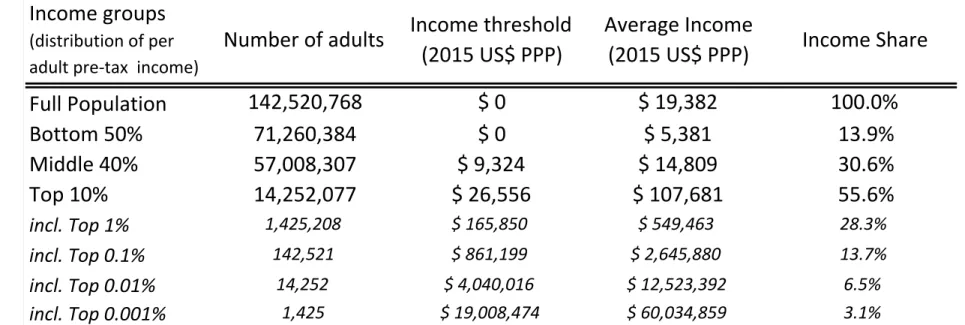
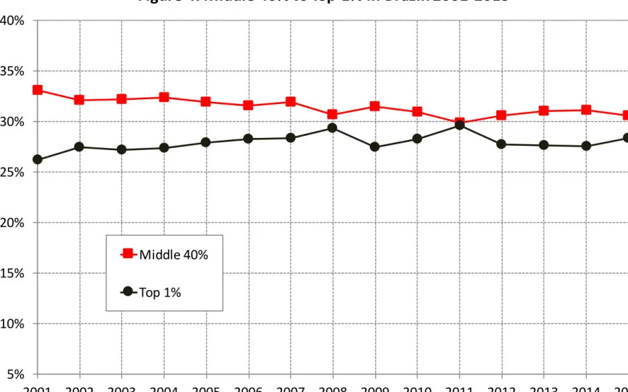
Figure 3 presents our corrected estimates for the full distribution of national income in Brazil, separating the adult population into the Top 10%, Middle 40% and Bottom 50%. The first finding to highlight is the extent of income concentration in Brazil. The richest 10% in the population receive around 55% of total income, while the bottom half in the population, a group five times larger, receives less than 15%. The Middle 40% in the distribution receives less than one third of total income, which is less than its proportional share. This reveals that inequality in Brazil is about the large division between the top and the rest of the income hierarchy. Second, the trends over the fifteen-year period show a resilient concentration at the top and a compression of the distribution within the bottom 90%. Despite the gains made by the Bottom 50%, which increased its share of national income from 12.6% to 13.9%, the Top 10% income share also evolved positively, from 54.3% to 55.6%. These gains came at the expense of a squeezed Middle 40%, whose share of income fell by the corresponding amount (2.5 percentage points) over the period. Therefore, while inequality among the bottom 90% declined, the top consolidated its concentration. Table 2 presents the income thresholds and averages for these income groups as well as for more refined shares at the top in 2015 US Dollars PPP. In this year, to be one of the richest
15 The missing 29% is made up of annual bonuses, the exempt portions of pensions and agricultural labour income, compensation for the termination of a contract, unemployment insurance, employer fringe benefits and payroll taxes, and any potential tax evasion/under-reporting.
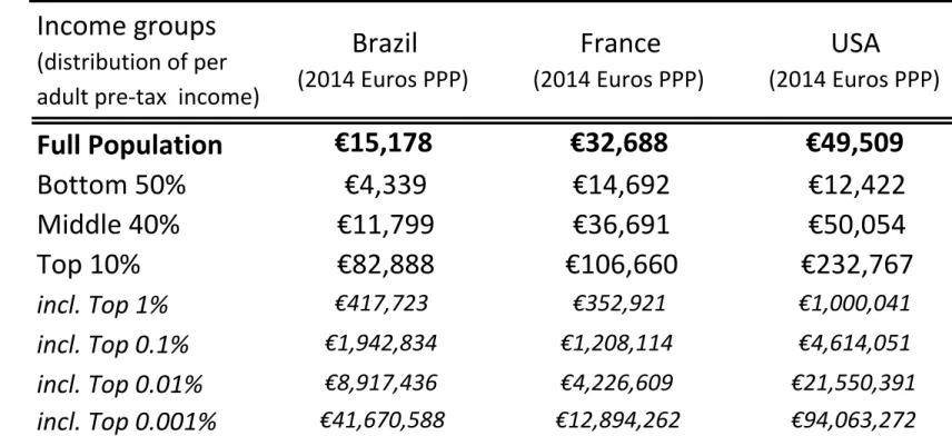
10% of adults in Brazil you need to make the equivalent of at least 26,556 dollars per year (almost 50,000 reais). The average income of the top decile was just over 107,000 dollars (almost 200,000 reais). The magnitudes increase substantially as we move into the top percentile of the distribution, with the average income of the richest 1% being around 550,000 dollars. Table 2.1 shows the average incomes of different groups in the population in Brazil compared to those in France and the USA in purchasing power parity Euros of 2014. The structure of inequality in Brazil depicts a country of two radically different societies. While Brazil is half as rich as France and less than one third as rich as the USA overall, there is an extremely rich group at the top with broadly comparable levels of pre-tax income (compared to France, Brazilian elites in the Top 1% and above have higher average incomes). However, while individuals at the top in Brazil are as rich as their counterparts in developed countries, the rest are much poorer. The average income of Brazil’s Middle 40% is below the average income of the Bottom 50% in both France and the USA. This conveys the lack of a broad “middle class” in Brazil’s dual social structure.16
Table 3 presents the 2015 shares for the same income groups and across our different income series previously defined. For instance, the Top 1% (about 1.4 million adults) in the surveys received 11% of income. However, when we correct top incomes using fiscal data and factor in undistributed income from national accounts the share increases dramatically to 24% in the fiscal income series and to 28% in the national income series. In other words, the top percentile commands 28 times the average income of the country.17 The large share captured by the Top 1% seems to be feeding from the Middle 40% share over time, as Figure 4 shows. Moving up the distribution the story is the same, with elites capturing disproportionate shares of total income. Figure 5 shows that the Bottom 50% (70 million adults) has comparable shares of income as the Top 0.1% (140,000 adults) over our time period. Starting at similar levels in 2001 both increased their shares over time, with the Bottom 50% subject to less volatility.
16 While the socio-economic concept of a “middle class” is salient in Brazil, it comprises a much smaller share of the population than in advanced economies. As a result, the “middle class” (as traditionally understood in developed countries – individuals in certain occupations, with certain employment security, lifestyles, etc.) is located closer to the top of the distribution than to the median in a country like Brazil, which squeezes the relative incomes of the middle 40% of the distribution. 17 If all adults earned the average income of their economy then the share of income of the Top 1% should be 1%. The fact that in Brazil this group concentrates about 28% of income equates to them having 28 times the average income per year.
Figures 6-9 plot the temporal comparison of the estimates from our three series: the raw estimates from the surveys, our corrected series for fiscal income (combining survey and fiscal data) and our benchmark national income (DINA) series (combining national accounts, surveys and fiscal data). In all cases, what the surveys allow us to estimate is a very distorted picture of reality. When compared to our benchmark national income series, the discrepancy is very large and increasing the higher up we move in the distribution. In general, the bulk of the correction is made from survey income to fiscal income using information from tax declarations.18 Therefore, relying exclusively on surveys or even ignoring undistributed income in national accounts flowing to corporates can distort the dynamics at play. For instance, according to the surveys inequality unequivocally fell over the last 15 years (the top shares fell, and the middle and bottom shares rose), while our national income series shows a more nuanced picture – an increase in concentration at the top, less of an increase at the bottom and an ever-squeezed middle over the period. At the same time, we provide stronger evidence that the inequality of labour earnings did fall, when using fiscal data to complement surveys. Figure 10 presents our shares of labour income for the full population when using income tax declarations to correct the top of the labour income distribution from the surveys (as described in section 2.4.3). The Top 10% labour income share fell steadily (by 4%), the Middle 40% stayed very stable, while the Bottom 50% labour income share increased considerably more than the national income series (18% vs 11%). Again, surveys seem to underestimate the dispersion in labour income (Figure 10.1), although by a lower magnitude than for total income (see Figures 6-8). The decline in “wage inequality” is more apparent if we focus on formal private sector employees using social contributions data. The Top 10% wage income shares falls three times as much as the share of total labour income (including pensions, informal and self-employed (autonomous/liberal professional), while the Bottom 50% share increased almost twice as fast (see Figure 11). The evolution is consistent with that observed using the raw survey data (Figure 11.1), but the levels are still more unequal. The clear picture that
18 The reason why the DINA shares for the Bottom 50% lie in between the survey income series and the fiscal income series (Figure 8), in contrast to what we see in the other Figures, is due to the equalizing effects of factoring in imputed rent and social security contributions across the full population for the national income distribution.
emerges from the analysis of these two distributions is that the Middle 40% is far less squeezed than in the total income distribution and that the evolution of formal earnings contributed a substantial positive element to the decline labour income inequality.
Figure 12 conveys the evolution of labour income and earnings among the Top 1%, compared to our benchmark national income series. While the levels of concentration at the top of our two labour income distributions is much less than the concentration in the total income distribution, their evolution followed a visible downward trend, again consistent with what the surveys show but along different levels (see Figure 12.1). This illustrates that the distribution of the returns to capital ownership played an important role in limiting the fall in total pre-tax inequality in Brazil. These findings are consistent with the evolution of the Gini coefficients, as depicted in Figure 13. Overall inequality fell, according to our corrected Gini and to the survey Gini, but does so more strongly for the survey income distribution. Given that surveys are more reliable in reporting labour incomes, this is unsurprising. But in addition, it must be noted that the Gini measure of inequality is less sensitive to movements in the tails of the distribution. This implies that it mostly captures changes in the distribution of labour earnings, given the deduced concentration of capital income in the right tail. It is thus also unsurprising that even our corrected Gini coefficient shows a slight decline over time. Section 4.2 discusses how we can understand these evolutions in the political context of the period.
Despite the fact that we are mainly interested here in the evolution of primary income inequality, before the intervention of government transfers (except social security pensions and unemployment insurance), we can perform a simple calculation to factor into our estimates the extent to which welfare cash transfers make a difference. Brazil’s cash transfers have received much media attention for their positive redistributive impact to the poor. Indeed, the published research on Brazil to date has placed much emphasis on the increased resources that have been dedicated to social assistance programs since the early 2000s (see Barros et al. 2010).
To better see their impact, we make the following calculation. From national accounts, we obtain the annual amount of social assistance cash transfers received by households. These
include Brazil’s flagship conditional cash transfer, Bolsa Familia, and welfare pensions for the elderly or incapacitated poor (Benefício de Prestação Continuada). Over our period of analysis these programs accounted for about 1% of national income, varying from 0.3% in the early 2000s to 1.5% by the end of the period. Given the difficulties in estimating the exact incidence of these transfers (due to them being financed out of general tax revenues) we proceed by calculating the maximum inequality reduction that can be achieved with the current values of the benefits. We thus assume that the entirety of these transfers flows to the Bottom 50% in the distribution and that they are paid from taxes on the Top 10%. This implies subtracting from the share of the Top 10% the share of transfers in national income and adding it to the share of the Bottom 50%. Our interest here is to show the maximum contribution of these transfers, at their present levels, to decrease inequality. The results of this calculation are presented in Figure 14. The share of the Bottom 50% increases from 13.9% to 15.4% in 2015, while the share of the Top 10% decreases from 55.6% to 54.1%. In addition, the growth rate of the share of the poorest 50% increases from 10% to 20% over the period when adding in the transfers, as their share in national income rose substantially. It can be seen that what matters for the income share poor is the size of these programs in national income. Although they make a big difference at the household level, in the aggregate distribution their contribution is still slim. The actual scenario is evidently more complex as the incidence of the taxes funding these programs may be more widely spread across the distribution, suggesting less redistribution than the “best-case scenario” presented above.
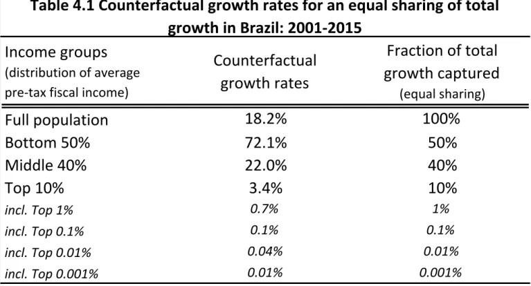
3.2. The Distribution of Growth and Recession
Between 2001 and 2015 the total cumulated real growth of national income per adult in Brazil was 18.2% (see Table 4). The question that arises from this evolution is how the average income growth of different income groups compares to these numbers. Consistent with evolution of income shares, the average income growth rate of the Bottom 50% was strong, compared to the Middle 40% and the Top 10%. The Middle 40% was the only group to grow at a rate less than the average for the whole population. Growth was also strong among the top percentiles with the income of the Top 1% growing by 28%, however this was still lower than the average growth registered by the poorest 50% over the period (30%).
Despite the gains made by the bottom, the top of the distribution continues to capture a disproportionate part of the income growth over the period, with the Top 10% capturing 63% of total average growth and the Top 1% capturing more than half of this (40% of total growth). The bottom line is that even with the strongest growth performance over the period, the Bottom 50% did not capture most of the growth due to their extremely low levels of income and their subsequently low share of income (13% on average for the entire period). Thus, over a short-to-medium run timeframe, the income growth of the poor seems to matter less than their share of total income of the period. This is partly why the 1.4 million richest adults in Brazil captured a higher fraction of total growth than the poorest 70 million Brazilians. For the Middle 40% it is their weak growth performance that makes the difference.
Table 4 also presents the growth incidence subdivided by time period. During the pre-global-crisis period (2001-2007), all groups experienced strong positive growth as the economy expanded rapidly, again with the Middle 40% growing less than the average. In this period, growth was strongest for the very top percentiles. Growth in the years between 2007 and 2015 was less strong and varied for the different groups in the population. Growth was negative for the richest groups, which mostly reflects the effect of the financial crisis for those with highly volatile capital incomes. For the richest 100,000 or so individuals, their real annual income in 2015 was lower than what it was in 2007. The final column of Table 4 shows how the income effects of the recent domestic recession, which affected Brazil’s economy more than the global financial crisis (see Figure 1), were distributed. Average national income fell by 6.5% between 2013 and 2015, but the decline was strongest for the Bottom 50% and Middle 40%, with their average income falling by 8%. On the other side, individuals above the Top 0.1% experienced positive growth on average over the domestic recession, in contrast to their experience of the international crisis.19 This confirms the view that domestic recessions have a stronger proportional impact on the poor than the affluent, at least over the short run, as the rich have more diversified income channels and more control over their final remuneration, as well as the remuneration of others.
19 By 2013, the average income of the Top 0.01% and Top 0.001% had still not returned to their 2007 level despite the continued domestic economic buoyancy (the growth of their average income was -9% and -25% respectively between 2007 and 2013). Growth only returned to individuals in these highest fractiles after the domestic recession hit.
Lastly, Table 4.1 presents the growth rates that would have been needed in order for all the income groups to have captured an equal share of total per adult growth since 2001. The counterfactual scenario shows that a transfer of per adult growth from the Top 10% to the lower fractiles would have been needed for this equal sharing to occur. The Top 10% would have needed to grow by 3% (instead of 21%), the Middle 40% by 22% and Bottom 50% by 72% (instead of 9% and 30% respectively). This would have evidently needed policies targeting greater pre-tax income growth for the bottom 90%, such as more and better-paid formal jobs, as well as more regulated income growth for the top, coming, for instance, from stricter collective bargaining arrangements in firms and more binding personal income taxes (on the latter see Morgan, 2017). 3.3. International Comparisons The income disparities in Brazil revealed in the previous section can be emphasized further if they are placed in an international comparative perspective, with countries currently with comparable estimates for national income shares covering the entire distribution. Figures 13-15 present the shares of national income going to the Top 10% (Figure 15), the Middle 40% (Figure 16) and the Bottom 50% (Figure 17) in Brazil, China, France, India, Russia and the USA over the last fifteen years. The inequality between the top and the rest in Brazil is even starker when compared to other countries. The Top 10% in Brazil consistently surpasses the share captured by the same group in all other countries, with the exception of India’s recent rise. The situation for the Middle 40% is the inverse, as the Brazilian share has fallen below one third of national income, a share only undercut by India’s in 2012/2013. Comparing the Bottom 50%, Brazilian shares have surpassed US levels since 2009, and are steadily approaching Asian levels. But they are still far from those of a developed European economy like France. Interestingly the evolution of the poorest half of Brazilian adults has been the opposite of that observed in the USA since the early 2000s. In sum, the Brazilian distribution is highly skewed, but the bottom seems to have made greater gains than in most other countries since the new millennium. Figure 18 presents the comparison of the Top 1% income share in Brazil and the same countries as the previous figures. While Top 1% shares
in all countries have clearly increased (with the exception of France and Russia), elites in Brazil continue to concentrate more national income than their foreign counterparts. The persistence and extremity of Brazil’s inequality places the country at the world inequality frontier.
4. Explaining the Recent Trends in Brazilian Inequality
To make sense of the evolution of inequality in Brazil since the early 2000s we must comprehend the economic and political contexts of this period. Our period of analysis covers four administrations – the latter part of Fernando Cardoso’s government until 2003, and the subsequent thirteen-year government of the Worker’s Party (PT), including two terms under President Lula da Silva and the first term and part of the second term of his successor, Dilma Rousseff. The period also covers the financial uncertainty in South America during 2002/2003, the global crisis of 2008/2009 and the domestic recession of 2014/2015. Between the years 2000 and 2015, according to the national accounts, Brazil’s economy expanded by 43%, with 83% of this growth accounted for by consumption spending (private consumption making up 63%) and only 17% coming from investment. Despite favourable terms of trade, net exports contributed close to 0%. On the production side growth was led mainly by commodity refinement, construction, and the expansion of employment in services. Since the late 1990s, in the context of the millennium development goals, poverty reduction became central to the agenda of governments in Brazil. With the election of the PT, this was given greater impetus. Their general discourse, which was mirrored in their policies, focused largely on the bottom of the distribution. Without modifying the ownership of capital in the economy, or reforming the tax system – in which company profit withdrawals, dividends and interests are exempt from the progressive income tax schedule, inherited fortunes across states are taxed at an average rate of about 4%, and greater fiscal burden is placed on consumers of basic goods and services – the policy focus of the PT centred around redistributing the proceeds of production through cash transfers and increasing the bargaining power of workers through unions and collective wage negotiations, anchored to