HAL Id: hal-01183542
https://hal.archives-ouvertes.fr/hal-01183542v2
Preprint submitted on 11 Jun 2018
HAL is a multi-disciplinary open access archive for the deposit and dissemination of sci-entific research documents, whether they are pub-lished or not. The documents may come from teaching and research institutions in France or
L’archive ouverte pluridisciplinaire HAL, est destinée au dépôt et à la diffusion de documents scientifiques de niveau recherche, publiés ou non, émanant des établissements d’enseignement et de recherche français ou étrangers, des laboratoires
Non-Parametric Inference of Transition Probabilities
Based on Aalen-Johansen Integral Estimators for Acyclic
Multi-State Models: Application to LTC Insurance
Quentin Guibert, Frédéric Planchet
To cite this version:
Quentin Guibert, Frédéric Planchet. Non-Parametric Inference of Transition Probabilities Based on Aalen-Johansen Integral Estimators for Acyclic Multi-State Models: Application to LTC Insurance. 2018. �hal-01183542v2�
Non-Parametric Inference of Transition Probabilities Based on
Aalen-Johansen Integral Estimators for Acyclic Multi-State
Models: Application to LTC Insurance
Quentin Guibert∗1,2 and Frédéric Planchet†1,2
1Univ Lyon, Université Claude Bernard Lyon 1, Institut de Science Financière et d’Assurances (ISFA),
Laboratoire SAF EA2429, F-69366, Lyon, France
2Prim’Act, 42 avenue de la Grande Armée, 75017 Paris, France
May 24, 2018
Abstract
Studying Long Term Care (LTC) insurance requires modeling the lifetime of individuals in presence of both terminal and terminal events which are concurrent. Although a non-homogeneous semi-Markov multi-state model is probably the best candidate for this purpose, most of the current researches assume, maybe abusively, that the Markov assumption is satis-fied when fitting the model. In this context, using the Aalen-Johansen estimators for transition probabilities can induce bias, which can be important when the Markov assumption is strongly unstated. Based on some recent studies developing non-Markov estimators in the illness-death model that we can easily extend to a more general acyclic multi-state model, we exhibit three non-parametric estimators of transition probabilities of paying cash-flows, which are of interest when pricing or reserving LTC guarantees in discrete time. As our method directly estimates these quantities instead of transition intensities, it is possible to derive asymptotic results for these probabilities under non-dependent random right-censorship, obtained by re-setting the system with two competing risk blocks. Inclusion of left-truncation is also considered. We con-duct simulations to compare the performance of our transition probabilities estimators without the Markov assumption. Finally, we propose a numerical application with LTC insurance data, which is traditionally analyzed with a semi-Markov model.
Keywords: Multi-state model; Aalen-Johansen integral; non-parametric estimator; non-Markov process; LTC insurance.
∗
Email: [email protected].
†
1
Introduction
Multi-state models offer a sound modeling framework for the random pattern of states experienced by an individual along time. These stochastic models are very flexible and can be adapted to many applications. In biostatistics (Hougaard, 1999; Hougaard, 2001; Andersen and Keiding,2002), this specification is generally used to model the transitions between states, defined as the occurrence of a disease or a serious event affecting the survival of an individual. For credit risk and reliability areas, this framework is transposed to account for the lifetime history of a firm or an item, see e.g. Lando and Skødeberg (2002) and Janssen and Manca (2007). For fifteen years, multi-state models have provoked a growing interest in the actuarial literature modeling the random pattern of states experienced by a policyholder during the contract period. In this context, transitions between states occur when an event triggers the payment of premiums and benefits. For health and life insurance modeling purposes, many papers develop comprehensive frameworks for pricing and reserving both with Markov or semi-Markov assumptions (Haberman and Pitacco,1998; Denuit and Robert,2007). Christiansen (2012) gives a wide overview of the use of multi-state models in health insurance, including Long Term Care (LTC) insurance, from an academic perspective. For that purpose, actuaries need to estimate the transition probabilities between states and additionally the transition intensities if a continuous underlying model is used. In practice, these probabilities may be adjusted to account for complex policy conditions (e.g. waiting periods and deferral periods).
Fitting multi-state models related to disability and LTC insurance with the available data is gen-erally done with regression approaches, in a manner similar to mortality models. Most approaches in the empirical literature resort to the Markov assumption, i.e. the transition to the next state depends only on the current state, see e.g. Gauzère et al. (1999), Pritchard (2006), Deléglise et al. (2009), Levantesi and Menzietti (2012), Fong et al. (2015) among others. This allows to keep calcu-lations simple, but the process ignores the effects of the past lifetime-path. This assumption is also often used, since the available data for fitting the model are rare with few fine details. However, it is clearly inappropriate when modeling the LTC claimants mortality, as the transition probabilities depend on the occurring age and the duration (or sojourn time) of each disease, and a semi-Markov model seems to be more relevant. In the actuarial literature, research about fitting non-Markov models is relatively scarce and focused mainly on disability data, which are generally fitted with parametric models, e.g. the so-called Poisson model (Haberman and Pitacco, 1998) or the Cox semi-Markov model (Czado and Rudolph, 2002). For a semi-Markov without any loop, the most common approach consists in estimating each crude transition intensity, as the ratio between the number of transitions from one state to another and the exposure at risk. Then, a Poisson regression model is applied on both one-dimensional and two-dimensional multiple decrements tables, along similar lines to the smoothing approaches developed for one or two-dimensional mortality tables, see e.g. Currie et al. (2004) on the use of generalized additive models or generalized linear mod-els for this purpose. As noted by Tomas and Planchet (2013), the LTC claimants mortality rates have a complex pattern that requires using flexible smoothing techniques such as p-splines or local methods. Recently for LTC insurance contracts, Biessy (2015) and Fuino and Wagner (2017) use semi-Markov models with a Weibull law for the duration time in disability states, which can be easily implemented and are quite flexible. The calculation of the transition probabilities is carried out in a third step by solving Kolmogorov differential equations based on the smoothed transition intensities.
In this paper, we focus on multi-state model with both multiple terminal (e.g. multiple causes of death) and non-terminal (e.g. competing diseases or degrees of disability) events without possibility of recovery, which is adapted to many LTC insurance specifications. This type of multi-state model contains at most two jumps, in connection with the future cash-flows of the contract, and can be represented by a semi-Markov process. However when estimating the model, the usual approaches
described above can fail as several assumptions are violated. First, the usual Markov assumption is likely to be wrong in disability states. Second, the semi-Markov structure can be questioned depending on how the data are observed. In an estimation framework with disability or LTC insurance data, the Markov assumption is actually lost when a policyholder become disabled, e.g. Alzheimer’s disease or other degenerative diseases. This entry date is generally unobserved as the insurer only records the entry date in a dependency state as settled contractually. As a consequence, the observed duration can differ from the sojourn time with a chronic pathology depending on how quick the disease is diagnosed. Thus, the estimated transition probability from the healthy state to this contractual disability state could be biased if the transition intensities of a semi-Markov model are calculated on the left censored duration times. Similar issues may appear when the multi-state process is affected by exogenous effects, e.g. unobserved heterogeneity. Finally, the crude intensities used in regression approaches are calculated using a discrete-time method as the ratio between the number of transitions and the exposure. For transitions from a disability state, this requires to define carefully a (entry age, age)-diagram or a (duration, age)-diagram. In most cases, yearly or monthly death rates are considered, but for LTC guarantees a finer timescale may be necessary for the first year after the entry into dependency. This is typically what happens for disabled insured suffering from a terminal cancer, as their monthly death rates just after the entry into dependency is around 30%. This required to use diagrams with different timescales leading to several steps when smoothing the crude rates, which is awkward.
To avoid these issues, we propose a direct non-parametric estimation framework with no Markov assumption focusing on transition probabilities as key quantities for actuaries. The terminology "di-rect" means that this method does not require to estimate the transition intensities in a first step. Definition of these key transition probabilities depends on the terms of the policy and they are specifically exhibited to compute, in discrete time, the price or the amount of reserve related to insurance liabilities. Considering targets adapted to a non-homogeneous semi-Markov specification in line with the contract clauses, our method gives relevant estimators for these probabilities with asymptotic properties, even when the Markov assumption is not satisfied. This avoid to introduce bias when specified a Markov or semi-Markov framework based on transition intensities, and allows the construction of confidence intervals for transition probabilities, which is not possible after imple-menting numerical techniques for the resolution of Kolmogorov differential equations. An additional feature of our approach is that it is not needed to specify a discretization grid as our method is adapted to continuous-time data, or to introduce a parametric assumption. From a practical point of view, our estimators can be used to perform model checking, e.g. analyze the goodness of fit of a regression model, in a manner similar to that used for checking a parametric model for the survival function with the Kaplan-Meier estimator for the construction of biometric tables in insurance. In that sense, we underline that our key quantities are not smoothed.
Our approach is based on recent alternatives to the canonical Aalen-Johansen estimator for transition probabilities, which is adapted to Markov multi-state models, which have been developed for some particular non-Markov models. For a progressive (or acyclic) illness-death model, Meira-Machado et al. (2006) propose direct non-parametric estimators based on a Kaplan-Meier integral representation. Estimators exhibited by Allignol et al. (2014) are very similar, but use competing risks techniques and allow for left-truncation. This first generation of estimators has been recently criticized as they are systematically biased if the support of the observed lifetime distribution of an individual is not contained within that of the censoring distribution. Alternatives are given by de Uña-Álvarez and Meira-Machado (2015) and Titman (2015) in a progressive illness-death model, as well as some other configurations. However, our aim differs from estimating usual transition probabilities P pXt“ j | Xs“ hq, where Xtdenotes the state of the insured at time t, as is generally
blocks which are nested to account for the progressive form of the process with right-censored data. With such a structure, our model can be viewed as a particular case of a bivariate competing risks data problem with only one censoring process. This structure requires considering Aalen-Johansen integrals for competing risks data (Suzukawa, 2002), instead of the Meira-Machado et al. (2006)’ Kaplan-Meier integral estimators. This allows to construct a first class of transition probabilities estimators that we enrich secondly with more efficient alternatives, following de Uña-Álvarez and Meira-Machado (2015). As insurance data are generally subject to left-truncation and right-censoring, this paper examines also how to adapt all these estimators in that context.
This paper is organized as follows. Section 2 introduces the modeling framework adapted to LTC insurance and defines transition probabilities for the rest of the paper. After defining Aalen-Johansen integral estimators, we derive in Section3three versions of the non-parametric estimators of the quantities under study. Their asymptotic properties are discussed, as well as the inclusion of left-truncation. Section 4 is devoted to a simulation analysis to assess the performance of our non-parametric estimators. We also assess the bias which appears when estimating a semi-Markov model based on data simulated with censored duration times. Application to real French LTC insurance data is proposed in Section5. The supplementary material describes in more details the underlying estimation framework and presents the asymptotic results of our estimators, as well as some additional simulation results.
2
Multi-state model for LTC insurance
We present a semi-Markov model for a LTC insurance contract in Section 2.1 with the aim of introducing key probabilities for actuarial purposes. The interest of focusing on a direct estimation procedure for these indicators is discussed in Section2.2, in particular regarding to the loss of the semi-Markov assumption.
2.1 A semi-Markov model for LTC insurance payments
Long Term Care (LTC) insurance is a mix of social care and health care provided on a daily basis, formally or informally, at home or in institutions, to people suffering from a loss of mobility and autonomy in their activities of daily life. In France for example, this guarantee is dedicated to elderly people who are partially or totally dependent and benefits are mainly paid as an annuity. Their amounts depend on the policyholders’ lifetime-paths and possibly on their degree of dependency (see e.g. Plisson,2009; Courbage and Roudaut,2011).
As for classical guarantees the payments defined by the contract depend on the pattern of health states experienced by the policyholder and the sojourn time in each state, we introduce in this section a particular semi-Markov model to describe his current state, see e.g. Christiansen (2012) or Buchardt et al. (2014) for a more general presentation on semi-Markov models in similar situations for life and health insurance. This framework is fairly general and allows considering most of LTC insurance specifications. The semi-Markov structure is a natural choice as the Markov assumption is generally not satisfied for LTC insurance contracts, see e.g. Denuit and Robert (2007) and Tomas and Planchet (2013). Using the payments process, our aim here is exclusively to exhibit transition probabilities which are key quantities to compute beyond the prospective reserves as the expected present value of the cash flows.
For the rest of the paper, we employ a particular multi-state structure with no recovery that we call acyclic. On a probability space pΩ, A, Pq, we consider a time-continuous stochastic process pXtqtě0 with finite state space S “ ta0, e1, . . . , em1, d1, . . . , dm2u, as defined by the contract, and
right-continuous paths with left-hand limits. This process represents the state of the policyholder at time t ě 0. The set te1, . . . , em1u contains m1 intermediary states or non-terminal events that
we associate to disability competing causes. The set td1, . . . , dm2u contains terminal events, i.e.
absorbing states such as straight death, lapse or death after entry in dependency. The state a0
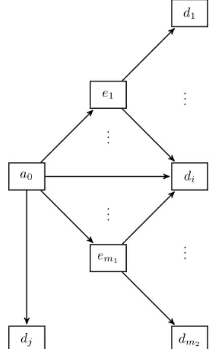
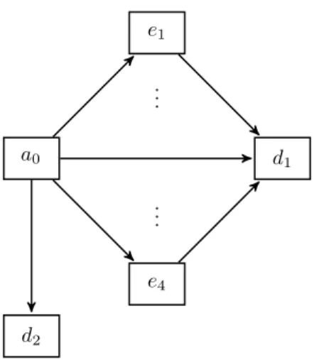
corresponds to the healthy state. Hence, an individual can take two types of lifetime paths depending on whether an intermediate event occurs or not. Figure 1 depicts an example of such an acyclical multi-state structurewith two levels of state considered in the LTC insurance contract.
e1 a0 em1 di d1 dm2 dj .. . .. . .. . .. .
Figure 1: Example of an acyclic multi-state model with intermediary and terminal states. We denote by pUtqtě0 the sojourn time spent in the current state
Ut“ max tτ P r0, ts : Xu “ Xt, u P rt ´ τ, tsu .
In such a context, it is natural to assume that the process pXt, Utqtě0 satisfies the Markov
assump-tion. The process pXtqtě0is then called a semi-Markov process and is characterized by the transition
probabilities, for all 0 ď u ď s ď t, v ě 0 and h, j P S
phjps, t, u, vq “ P pXt“ j, Utď v |pXs, Usq “ ph, uq q . (2.1)
We also define the transition intensities for all 0 ď u ď t and h, j P S, µhjpt, uq “ lim δtÑ0 phjpt, t ` δt, u, 8q δt for h ‰ j and µhhpt, uq “ ´ ÿ j‰h µhjpt, uq , (2.2)
which we suppose exist and are continuous. Note in particular that any acyclic multi-state model as in Figure 1 is a semi-Markov model, if X is endogenously generated. Finally, we introduce ¯
phhps, t, uq as the probability to not stay in state h within rs, ts with duration u in time s and use
the letter ∆ to indicate that the sojourn time is included into a time interval such as phjps, t, ∆u, ∆vq “ P pXt“ j, v ´ 1 ă Utď v | Xs“ h, u ´ 1 ă Us ď uq ,
and
¯
Under this semi-Markov framework , we can derive premiums and reserves expressions related to a LTC insurance policy. For that, we recall the general formula of the expected present value of benefits, net of premiums, paid within a period rt, 8r for a policyholder initially in state h P ta0, e1, . . . , em1u with duration u Vhpt, uq “ ż8 t δ pt, τ qÿ jPS żτ ´t`u 0 phjpt, τ, u, dvq ¨ ˝dBjpτ, vq ` ÿ l‰j µjlpτ, vq bjlpτ, vq ˛ ‚dτ , (2.3) where δ pt, τq “ e´ştτrsds, r
tdenotes the continuous compounded risk free interest rate, dBjpt, Utq “
bjpt, Utq dtis a continuous, net of premiums, annuity rate payments accumulated in state j during
the sojourn time Ut to the policyholder at time t. bjlpt, Utq is the single payment related to the
transition from state j to state l. The payments and the interest rate functions are assumed to be continuous and deterministic. Of course, when a insured reaches a state td1, . . . , dm2u, prospective
reserves are nil after the payment of the last benefits. Depending upon contractual conditions, the net benefits can easily include deferred periods and a stopping time.
Equation (2.3) can be differentiated with respect to t and u as a generalized Thiele’s differential equation (Hoem, 1972; Denuit and Robert, 2007). A common used method to derive prospective reserves with the Thiele equation consists in calculating the transition probabilities, given that the transition rates are specified, with the so-called Kolmogorov’s backward or Kolmogorov’s forward differential equations (see e.g. Buchardt et al.,2014).
In our particular case where the multi-state structure does not admit any loop (or any re-turn to a previous state) and only two jumps, computing procedures are simplified. In particu-lar, phhpt, τ, u, dvq, h P ta0, e1, . . . , em1u are zero for v ‰ τ ` u ´ t, otherwise phhpt, τ, u, dvq “
1 ´ ¯phhpt, τ, uq. Since the states d1. . . , dm2 are terminal states, a payment may occur only at the
transition time. Thus, we get Va0pt, uq “ ż8 t δ pt, τ q p1 ´ ¯pa0a0pt, τ, uqq dBa0pτ, τ ´ t ` uq dτ ` ż8 t δ pt, τ q p1 ´ ¯pa0a0pt, τ, uqq ÿ l‰a0 µa0lpτ, τ ´ t ` uq ba0lpτ, τ ´ t ` uqdτ ` ż8 t δ pt, τ q em1 ÿ j“e1 żτ ´t 0 pa0jpt, τ, u, dvq ¨ ˝dBjpτ, vq ` ÿ l‰j µjlpτ, vq bjlpτ, vq ˛ ‚dτ , (2.4) and, for e P te1, . . . , em1u Vept, uq “ ż8 t δ pt, τ q p1 ´ ¯peept, τ, uqq dBepτ, τ ´ t ` uq dτ ` ż8 t δ pt, τ q p1 ´ ¯peept, τ, uqq dm2 ÿ l“d1 µelpτ, τ ´ t ` uq belpτ, τ ´ t ` uqdτ . (2.5)
In many practical situations, a discrete time approach is chosen to derive the prospective reserves, by assuming that transitions only happen at integer times (only one transition per period) and payments are null at non-integer times. For simplicity and without a significant loss of generality, we suppose the payments and transitional probabilities from the state a0 do not depend on the
in discrete time (with a time-scale of 1) with payments in advance and a sojourn time in state a0 equal to 0 Va0pt, 0q “ 8 ÿ τ “t δ pt, τ q p1 ´ ¯pa0a0pt, τ, 0qq pBa0pτ q ´ Ba0pτ ´ 1qq ` 8 ÿ τ “t δ pt, τ ` 1q p1 ´ ¯pa0a0pt, τ, 0qq ÿ l‰a0 pa0lpτ, τ ` 1, 0, 8q ba0lpτ ` 1q ` 8 ÿ τ “t`1 δ pt, τ q em1 ÿ j“e1 τ ´t ÿ v“1 pa0jpt, τ, 0, ∆vq pBjpτ, vq ´ Bjpτ ´ 1, v ´ 1qq ` 8 ÿ τ “t`1 δ pt, τ ` 1q em1 ÿ j“e1 τ ´t ÿ v“1 ÿ l‰j qa0jlpt, τ, 0, ∆vq bjlpτ, vq , (2.6) where pa0jpt, τ, 0, ∆vq “ P pXτ “ j, v ´ 1 ă Uτ ď v | Xt“ a0q ,
is the transition probability from state a0 to state j between time t and time τ and with a sojourn
time into ∆v “ sv ´ 1, vs, and
qa0jlpt, τ, 0, ∆vq “ P pXτ “ j, Xτ `1 “ l, v ´ 1 ă Uτ ď v | Xt“ a0q,
is the transition probability from state a0 to state l between time t and time τ and with a sojourn
time in an intermediary state j between v ´ 1 and v 1. Similarly, Equation (2.5) becomes for
e P te1, . . . , em1u Vept, uq “ 8 ÿ τ “t δ pt, τ q p1 ´ ¯peept, τ, ∆uqq pBepτ, τ ´ t ` uq ´ Bepτ ´ 1, τ ´ 1 ´ t ` uqq ` 8 ÿ τ “t δ pt, τ ` 1q p1 ´ ¯peept, τ, ∆uqq dm2 ÿ l“d1 pelpτ, τ ` 1, ∆τ ´t`u, 8q belpτ ` 1, τ ` 1 ´ t ` uq. (2.7) With the above discretized prospective reserves, we are interested in estimating probabilities of paying (or receiving) cash-flows:
i. p¯a0a0ps, t, 0q, 0 ď s ď t,
ii. pa0jps, t, 0, 8q, for a state j ‰ a0 and 0 ď s ď t,
iii. pa0eps, t, 0, ∆vq, for a non-terminal state due to cause e, 0 ď s ď t and a sojourn time into
∆v “ sv ´ 1, vs, v ě 0,
iv. qa0edps, t, 0, ∆vq, for a non-terminal state due to cause e, a terminal cause d, 0 ď s ď t and a
sojourn time in state e within ∆v “ sv ´ 1, vs, v ě 0,
v. p¯eeps, t, ∆uq, with a non-terminal event e and 0 ď u ď s ď t,
vi. pedps, t, ∆u, 8q, for a non-terminal event e, a terminal event d and 0 ď u ď s ď t.
1For the sake of simplicity, we use the same time interval to discretize the process along the time and the duration
2.2 Discussion on the estimation approach
For the semi-Markov framework introduced above, the transition probabilities could be easily carried out by solving Kolmogorov differential equations in continuous time based on the estimates of transition intensities. The latter are usually fitted by means of a Poisson regression model or a parametric model (e.g. Weibull duration laws). In this paper, we have chosen to estimate directly these probabilities, i.e. without using the transition intensities, and without any Markov assumption. Several motivations are discussed below.
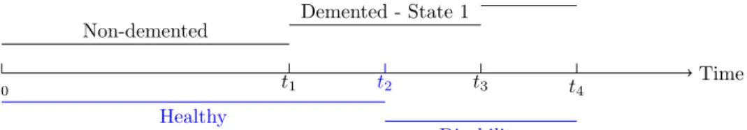
About the semi-Markov assumption As the definition of the state space S is in line with the contract clauses, the use of the semi-Markov model X might introduce bias in practical situations. In the LTC insurance context where a insured is exposed to progressive illnesses, such as Alzheimer’s disease, it is reasonable to assume that his health is influenced by several intermediary states (see e.g. Salazar et al., 2007). In particular, the sojourn time in each intermediary state may be a good candidate for explaining the evolution of the health state. However, these states could remain unobserved from the insurer’s point of view as individual data collected by insurance companies are incomplete and ignore usually the medical information. This situation is illustrated in Figure2
with the introduction of latent states influencing the current health state of the insured.
t0 Non-demented t1 Demented - State 1 t4 Healthy t2 Disability t3 Demented - State 2 Time
Figure 2: Example of follow-up of one insured. The blue lines represent the time spend in each observed state, as defined by the contract. The black lines is for the sojourn time in some
intermediary states related to a cognitive disease, e.g. dementia.
In this example, the insured is seen healthy by the insurer at time t1 and the claim is reported
at time t2, whereas the insured is actually demented for a duration time of t2´ t1. In addition,
the insurer ignores the transition to a more severe dementia state at time t3, which may affect the
occurrence of the death at time t4. In such a situation, the duration time in the disability state is
probably not enough to capture the dynamic of the process. Hence, a semi-Markov multi-state model based on an extended state space would be more relevant than a model based on contractual states. However, this extended state space is unattainable since the transition times into the intermediary states are unobserved. Our non-Markov approach is one way to solve this problem, as shown in Section4.2.
An alternative procedure for model checking The robustness of usual approaches depends on the quality of the transition intensities defined in two dimensions. Both for a parametric model and a Poisson regression model, this requires to compute crude intensity rates for analyzing the goodness-of-fits. These rates are based on a piecewise constant hypothesis on a durationˆage rectangle or on a durationˆentry age parallelogram. With individual data, the both versions are available. Estimating the crude intensity rates requires to define carefully the timescales used for aggregating along two dimensions the number of transitions and the contributions to the exposure at risk. In most cases, yearly or monthly rates are considered, but as an expert opinion. Our approach avoid to choose an arbitrary timescale, which is appealing for model checking. In addition, our estimators
allow to focus directly on the transition probabilities of interest and not on the transition intensities which can be seen as intermediary outcomes. Another argument is that our approach allows us to derive asymptotic properties for the estimates, which is not possible when estimating the transition intensities and then resolving the Kolmogorov differential equations.
3
Non-parametric estimation of transition probabilities
This section outlines in 3.1 our notations and explains the link between transition probabilities of interest and a bivariate competing risks structure for estimation purposes. We do this in a heuristic fashion for right-censoring data and give more details regarding the underlying framework, the asymptotic properties of the estimators and the related proofs in the supplementary material. In particular, this material discusses the case where discrete covariates are added. Section 3.2
investigates alternative estimators to the first approach avoiding systematic biases and improves efficiency. Proofs are also available in the supplementary material. As LTC insurance data are also subject to left-truncation, we ultimately explain in Section3.3how to adapt our estimators to comply with it.
3.1 Estimation with Aalen-Johansen integrals
In case the process is Markovian, transition probabilities of interest do not depend on the sojourn time in a disability state and can be estimated non-parametrically with the so-called Aalen-Johansen estimator (Aalen and Johansen, 1978; Andersen et al., 1993). However, this methodology fails when the Markov assumption is wrong, especially when these probabilities depend on both time and duration (semi-Markov models). In what follows, we develop a non-parametric approach to estimate directly these transition probabilities, instead of calculating transition intensities.
The proposed estimation approach for acyclic multi-state models is based on two competing risks processes which are nested. In a first step, the individual lifetime history can be affected by competing exit-causes from the healthy state, i.e. to the non-terminal (a0 Ñ e) and to the terminal
(a0 Ñ d) states. In a second step, the residual lifetime is exposed to m2-causes of exit, may they
be direct (a Ñ d) or indirect through one of the m1 intermediary states (a Ñ e Ñ d).
Let pS, V1qand pT, V q be two competing risk models, where S is the sojourn time in the healthy
state a0, V1 indicates the exit cause of the state a0, T is the overall survival time and V “ pV1, V2q
with V2 indicating the reached absorbing state. As noted by Meira-Machado et al. (2006) with
an acyclic illness-death model, S “ T and V1 is identical to V2 when a direct transition occurs
initially. Otherwise, we have S ă T and V1 codes necessarily an intermediary state. Note also that
V2 depends on the value taken by V1, in accordance with the multi-state structure.
The data used for estimation are subject to censoring and the two lifetime variables pS, T q are not directly observed. We consider a right censoring variable C, which is assumed to be independent to the vector pS, T, V q. This assumption is widely used for simplicity in practice and is generally verified by insurance data as observations are censored by administrative events or simply due to the end of the observation period. It is important to note that the censoring variable is unique. Thus, the following variables are available
#
Y “ min pS, Cq and γ “ 1tSďCu,
Z “ min pT, Cq and δ “ 1tT ďCu.
The observation of the i-th individual of a sample of length n ě 1 is characterized by pYi, γi, γiV1,i, Zi, δi, δiV2,iq 1 ď i ď n ,
which are assumed to be i.i.d. replications of the variable pY, γ, γV1, Z, δ, δV2q. If δ “ 1, then
obviously γ “ 1. Thus, the transition probabilities of interest can be expressed in terms of the joint distributions pS, V1q and pS, T, V q as follows
¯ pa0a0ps, t, 0q “ P ps ă S ď tq P pS ą sq , (3.1) pa0jps, t, 0, 8q “ P ps ă S ď t, V1 “ jq P pS ą sq , (3.2) pa0eps, t, 0, ∆vq “ P ps ă S ď t ă T , t ´ S P ∆v, V1 “ eq P pS ą sq , (3.3) qa0edps, t, 0, ∆vq “ P ps ă S ď t ă T ď t ` 1, t ´ S P ∆v, V “ pe, dqq P pS ą sq , (3.4) ¯ peeps, t, ∆uq “ P pS ď s ă T ď t, s ´ S P ∆u, V1 “ eq P pS ď s ă T , s ´ S P ∆u, V1“ eq , (3.5) pedps, t, ∆u, 8q “ P pS ď s ă T ď t, s ´ S P ∆u, V “ pe, dqq P pS ď s ă T , s ´ S P ∆u, V1 “ eq . (3.6)
Even if the Markov assumption is not verified, the probability (3.1) can be simply estimated using the Kaplan-Meier estimator of the distribution function of S, noted H and assumed to be continuous p Hnpsq “ n ÿ i“1 Win1tYi:nďsu, (3.7)
where Y1:n ď Y2:n ď . . . ď Yn:n is the ordered Y -values, γri:ns the concomitant of the i-th order
statistic (i.e. the value of pγjq1ďjďn paired with Yi:n) and
Win “ γri:ns n ´ i ` 1 i´1 ź j“1 ˆ n ´ j n ´ j ` 1 ˙γrj:ns ,
the Kaplan-Meier weight for the the i-th ordered observation. An estimator of the numerator in Equation (3.2) is obtained considering the Aalen-Johansen estimator for competing risks data of the cumulative function Hpeq
psq “ P pS ď s, V1 “ eq, i.e. p Hpeq n psq “ n ÿ i“1
Winpeq1tYi:nďsu, (3.8)
where Wpeq
in “ Win1tV1,ri:ns“eu.
Other probabilities include more complex terms which depend on pS, T, V q. By defining the bivariate cumulative incidence function (assumed to be continuous)
Fpe,dq
ps, tq “ P pS ď s, T ď t, V “ pe, dqq , s ď t,
these complex terms can be expressed as integrals of the form ş ϕ dFpe,dq, where ϕ is a simple
transformation of S and T . This bivariate cumulative incidence function is defined and estimated nonparametrically by Cheng et al. (2007) under independent right-censoring. However, their rep-resentation is devoted to general bivariate competing risks data and we aim to provide estima-tors which exploit the information that S is necessarily observed when T is not censored. For
this purpose, it is convenient to introduce Z1:n ď Z2:n ď . . . ď Zn:n the ordered Z-values and ´ Yri:ns, δri:ns, J pe,dq ri:ns ¯
the concomitant of the i-th order statistic with Jpe,dq
i “1tVi“pe,dqu.
Based on the idea of Meira-Machado et al. (2006), we consider S as a covariate and estimate Fpe,dqusing the so-called Aalen-Johansen estimator (Aalen and Johansen,1978) adapted to a single
competing risks model. This estimator can be written as p Fpe,dq n py, zq “ n ÿ i“1 Ă Winpe,dq1tY
ri:nsďy,Zi:nďzu
“ n ÿ i“1 Ă WinJri:nspe,dq1tY
ri:nsďy,Zi:nďzu,
(3.9)
where ĂWindenotes the Kaplan-Meier weight of the i-th ordered observation, related to the estimated
survival function of T . The Aalen-Johansen weights for states pe, dq, defined as Ă Winpe,dq “ δri:nsJ pe,dq ri:ns n ´ i ` 1 i´1 ź j“1 ˆ n ´ j n ´ j ` 1 ˙δrj:ns , 1 ď i ď n,
are very close to the Kaplan-Meier weights related to the estimated survival function of T . They can be interpreted as the mass associated to one observation. We also denote Jpeq
i “1tV1,i“eu and
Ă
Winpeq“řdi“1m2WĂinpe,diq2.
Note that the Inverse Probability of Censoring Weighting (IPCW) representation can be easily derived from this expression by writing3
Ă Winpe,dq“ δri:nsJ pe,dq ri:ns n´1 ´ pGnpYi:nq ¯ ,
where pGn represents the Kaplan-Meier estimator of the distribution function of C. The IPCW
theory is largely used for survival models with dependent censoring and was recently applied to state occupation, exit and waiting times probabilities for acyclic multi-state models (Mostajabi and Datta,2013) and to transition probabilities for the illness-death model (Meira-Machado et al.,
2014). The extension of our estimators with these regression techniques would be clearly feasible here, but is out of the scope of this paper.
Based on the representation as a sum of (3.9), we are now interested in obtaining estimators for probabilities (3.3-3.6). Since the joint distribution of pT, V q has the aspect of a competing risks model, we propose the following estimators
p
pa0eps, t, 0, ∆vq “
řn
i“1ĂWinpeq1
tsăYri:nsďtăZi:n, t´Yri:nsP∆vu
1 ´ pHnpsq , (3.10) p qa0edps, t, 0, ∆vq “ řn i“1WĂinpe,dq1
tsăYri:nsďtăZi:nďt`1, t´Yri:nsP∆vu
1 ´ pHnpsq , (3.11) p ¯ peeps, t, ∆uq “ řn i“1ĂWinpeq1
tYri:nsďsăZi:nďt, s´Yri:nsP∆uu
řn
i“1ĂWinpeq1
tYri:nsďsăZi:n, s´Yri:nsP∆uu
, (3.12)
2
Of course tV1“ eu “ tV1“ e, V2P td1, . . . , dm2uu “ tV1“ e, V2P C pequ, where C peq is the set of states to which
a direct transition from e is possible.
3
p
pedps, t, ∆u, 8q “
řn i“1WĂ
pe,dq
in 1tYri:nsďsăZi:nďt, s´Yri:nsP∆uu
řn i“1ĂW
peq
in 1tYri:nsďsăZi:n, s´Yri:nsP∆uu
. (3.13)
As Y is considered as an uncensored covariate when T is not censored, these estimators are consistent w.p.1, if the support of Z is included in that of C, and they verify consistency and weak convergence properties. To obtain these results with independant right-censoring, we derive general asymptotic properties for Aalen-Johansen integrals estimators with competing risks data by refining the estimators exhibited by Suzukawa (2002) with the addition of covariates.
The asymptotic variance functions of these estimated transition probabilities are tricky to infer. To get around this difficulty, bootstrap or jackknife techniques can be used. In section5, we con-struct non-parametric bootstrap pointwise confidence bands for our estimators. This is done with a simple bootstrap resampling procedure (Efron,1979). Although it seems that jackknife techniques performs well (Azarang et al.,2015), bootstrap approaches are often preferred for practical applica-tions as their computation cost is lower, especially when the amount of data is significant. Note also that Beyersmann et al. (2013) provide wild bootstrap approach for the Aalen-Johansen estimator for competing risks data but, as it is remarked in their paper, this approach is quite close to that followed by Efron. To the best of our knowledge, no further tentative has been proposed to ob-tain more consistent bootstrap methodologies for cumulative intensity function or other transition probabilities.
Finally, remark that we could write probabilities (3.2) for j P td1, . . . , dm2u as
P ps ă S, T ď t, V1“ V2 “ jq
P pS ą sq .
In this case, these probabilities would be estimated using Aalen-Johansen integrals estimators, which are consistent at time t in the support of Z. Thus, the Aalen-Johansen weights would be involved instead of the Kaplan-Meier weights related to S. Considering the estimator (3.8) is equivalent to apply right-truncation on the observations which experience non-terminal events. However, we prefer this approach as it preserves the relation ¯pa0a0ps, t, 0q “
ř
j‰a0pa0jps, t, 0, 8q. This seems
more relevant for actuarial applications.
3.2 Alternative estimators
Although they verify asymptotic properties, the main drawback of the previous estimators is that they are systematically biased if the support of Z is not contained within that of the right-censoring distribution. This situation is rather restrictive and some alternative estimators have been recently proposed. de Uña-Álvarez and Meira-Machado (2015) introduce new estimators of transitional probabilities, P pXt“ j | Xs “ hq of an illness-death model, which cope with this issue. One of
their estimators is a conditional Pepe-type estimator (Pepe, 1991), i.e. the difference between two Kaplan-Meier estimates. Titman (2015) gives estimators for transitional probabilities between states or sets of states which may be used with a non-progressive multi-state model for particular transitions.
Our methodology to find alternative estimators adapts the approach developed by de Uña-Álvarez and Meira-Machado (2015) to complex transition probabilities (3.3-3.6) in an acyclic multi-state model. Following these authors, two alternative estimators are exhibited. By remarking for Equations (3.4) and (3.5) that
qa0edps, t, 0, ∆vq “ P pXt“ e, Xt`1“ d, v ´ 1 ă Utď v | Xs“ a0q
“ P pXt`1“ d | Xs“ a0, Xt“ e, v ´ 1 ă Utď vq P pXt“ e, v ´ 1 ă Utď v | Xs“ a0q
if t ´ s ą v by construction, and ¯peeps, t, ∆uq “ řmi“12 pedips, t, ∆u, 8q, we limit our analysis and
especially focus on estimating quantities (3.3) and (3.6).
The first solution consists in rewriting pa0eps, t, 0, ∆vq and pedpt, t ` 1, ∆v, 8q
p p˚ a0eps, t, 0, ∆vq “ řn i“1W peq
in 1tsăYi:nďt, t´Yi:nP∆vu´
řn
i“1WĂinpeq1
tsăYri:ns,Zi:nďt, t´Yri:nsP∆vu
1 ´ pHnpsq
, (3.14) which is consistent to pa0eps, t, 0, ∆vqand asymptotically normal, when max pt, t ´ v ` 1q is included
in the support of Y (see the left term of the numerator), and
p p˚ edps, t, ∆u, 8q “ řn i“1WĂ pe,dq
in 1tYri:nsďsăZi:nďt, s´Yri:nsP∆uu
řn
i“1W
peq
in 1tYi:nďs, s´Yi:nP∆uu´
řn i“1WĂ
peq
in 1tYri:nsďs,Zi:nďs, s´Yri:nsP∆uu
, (3.15)
which is consistent when t is included in the support of Y or when max ps, s ´ u ` 1q and t are respectively included in those of Y and Z4.
To increase efficiency of the estimators introduced by Meira-Machado et al. (2006), Allignol et al. (2014) construct new estimators for P pXt“ j | Xs“ hq by restricting the initial sample of
length n to the subpopulation at risk in state h at time s. Titman (2015) and de Uña-Álvarez and Meira-Machado (2015) follow a similar restriction. In our case, we consider first the subset ti : Yią su with cardinal snand estimate pa0eps, t, 0, ∆vq as
q
pa0eps, t, 0, ∆vq “ sn
ÿ
i“1
sWipeqsn1tsYi:snďt, t´sYi:snP∆vu
´ sn ÿ i“1 sWĂ peq
isn1tZi:snďt, t´Yri:snsP∆vu,
(3.16)
wheresY is the lifetime in the initial state for individuals who were still in this state at time s. We
introduce by analogysWipeqsn,sWĂ
peq
isn and sZ.
Second, we select individuals in the subset ti : Yiă s ď Zi, s ´ YiP ∆uu of cardinals,un. With
this selection and unambiguous notations, pedps, t, ∆u, 8qcan be estimated with
q pedps, t, ∆u, 8q “ s,un ÿ i“1 s,uĂW pe,dq
is,un1ts,uZi:s,unďtu. (3.17)
This corresponds to the Aalen-Johansen estimators for the cumulative incidence function of a com-peting risks model based on a particular subsample. Note that if there is only one terminal state which can be reached from e, Equation (3.17) corresponds to the Kaplan-Meier estimator of the distribution function of T conditionally on tY ă s ď Z, s ´ Y P ∆uu.
Similarly to the initial estimators considered in Section 3.1, bootstrap resampling techniques can be used to estimate the variance of these alternative estimators.
3.3 Estimation under right-censoring and left-truncation
Insurance datasets are often subject to left-truncation (e.g. the subscription date of the contract) and censoring together. Up to now, the proposed estimators are defined only under right-censoring. We discuss in this Section how to address this issue.
4
Due to the nested structure of the model, only one truncation variable L should be considered. Hence, Y and Z are observed if Y ě L. For LTC insurance data, which is studied in Section 5, left-truncation always occurs when the individual is still in the healthy state. This situation seems to make sense for health insurance applications, as the insurer accepts only non-dependent policy-holders at the subscription date. For this reason, we exclude here more complicated situations that may arise in a more general framework if the left-truncation events occur after S (see e.g. Peng and Fine,2006, for an illness-death model).
In this manner, we refine our proposed estimators for left-truncated and right-censored data following the representation defined by Sánchez-Sellero et al. (2005). To be specific, we assume that pC, Lqis independent of pS, T, V q and C is independent of L. As we have n i.i.d. observations
pYi, γi, γiV1,i, Zi, δi, δiV2,i, Liq , i “ 1, . . . , n,
only if Li ď Yi, we redefine respectively the Kaplan-Meier and the Aalen-Johansen weights such as
Win:“ γi nCnpYiq ź tj:YjăYiu ˆ 1 ´ 1 nCnpZjq ˙γj , and Ă Winpe,dq :“ δiJ pe,dq i n rCnpZiq ź tj:ZjăZiu ˜ 1 ´ 1 n rCnpZiq ¸δj , where Cnpxq “ n´1 řn
i“11tLiďxďYiu and rCnpxq “ n
´1řn
i“11tLiďxďZiu. Then, these weights can
be replaced in Equations (3.7-3.15) to obtain new estimators which are almost surely consistent and asymptotically normal if, in addition, the largest lower bound for the support of L is lower than that of S and P pL ď Sq ą 0. Estimators (3.16) and (3.17) can be adjusted in a similar way, i.e. by considering the subset ti : Yi ą su and ti : Yi ă s ď Zi, s ´ YiP ∆uu, and then the weights
pertaining to these subsamples. In this manner, we need to verify than the number of individuals at risk is not nil with a positive probability. Additional information regarding the asymptotic results are given in the supplementary material.
4
Simulation results for transition probabilities
In this section, we deploy a simulation approach to assess the performance of our proposed estima-tors. As noted above, we focus on probabilities (3.3) and (3.6). Two sets of simulations are done, comparing our estimators between them and with a semi-Markov model.
The computations are carried out with the software R (R Core Team, 2017). As our model is based on competing risks models, the R-package mstate designed by De Wreede et al. (2011) and the book of Beyersmann et al. (2011) give useful initial toolkits for the development of our code. Note that the model provided by Meira-Machado et al. (2006) is also implemented in R (Meira-Machado and Roca-Pardinas, 2011). We also use the package SemiMarkov for fitting an homogeneous semi-Markov model (Król and Saint-Pierre,2015). Our script is available upon request made to the first author.
4.1 Comparison of the proposed estimators
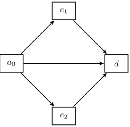
The aim of this section is to compare the performance of the non-parametric estimators introduced above. For that, we introduce the multi-state structure depicted in Figure 3. For the sake of simplicity and without loss of generality, we consider only one terminal event and two non-terminal
events. Let Ta0e1, Ta0e2 and Ta0d be the latent failure times in healthy state a0 corresponding to
the non-terminal states te1, e2uand to the absorbing state d. We also set Te1dand Te2dthe residual
lifetime from each non-terminal state due to cause d.
e1
a0
e2
d
Figure 3: Multi-state structure for the simulation study.
To simulate a non-Markov process, we specify a dependence assumption between each latent failure times and consider the simulation approach set up by Rotolo et al. (2013).
First, we set a Clayton copula Cθ0 with dependent parameter θ0 to combine the failure times
Ta0e, e P te1, e2u, and Ta0dfrom the starting state a0
P pTa0e1 ą te1, Ta0e2 ą te2, Ta0dą tdq “ Cθ0pP pTa0e1 ą te1q , P pTa0e2 ą te2q , P pTa0dą tdqq “ ¨ ˝1 ` P pTa0dą tdq´θ0 ` ÿ ePte1,e2u ” P pTa0eą teq ´θ0 ´ 1 ı ˛ ‚ ´1{θ0 . As a second step, we define another Clayton copula Cθe for each non-terminal event e1, e2 to put
together its latent times Ta0e and its children’s Ted. This gives for e P te1, e2u
P pTa0eą te, Ted ą tdq “ CθepP pTa0eą teq , P pTedą tdqq “ ´ 1 ` P pTa0eą teq ´θe ` P pTed ą tdq´θe ¯´1{θe .
With this setting, we assume the dependent parameters θ0 and θe, e P te1, e2u, have the same
value θ “ 0.5 for each copula model. The latent failure times Ta0e, Ted, e P te1, e2u, and T0d are
generated with Weibull distributions Wei pλ, ρq, where λ and ρ being respectively the scale and shape parameters. Parameters are selected in order to have features similar to that of a sample of LTC claimants. Table1 presents the selected parameters.
To assess the performance of our estimators, we compare the results under two censoring sce-narios: C follows an independent Uniform distribution U r30, 45s (Scenario 1), and an independent Weibull distribution Wei p80, 1q (Scenario 2), i.e. an Exponential distribution. With this specifica-tion, the proportion of censoring for Scenario 1 is 14% (24% for Scenario 2) for individuals in state a0, 33% (30% for Scenario 2) for individuals reaching the state e1 and 38% (28% for Scenario 2)
for those experiencing the state e2. For Scenario 1, we choose the window r30, 45s as many
transi-tions to states e1 and e2 occur during this period. In this respect, the aim is to reveal the lack of
performance of estimators introduced in Section3.1. For each scenario, we consider three samples with size n “ 100, n “ 200 and n “ 400. For e P te1, e2u, we compute pa0eps, s ` 4, 0, ∆vq and
Table 1: Simulation parameters used for the failure latent times.
Parameter Ta0e1 Ta0e2 Ta0d Te1d Te2d
Scale λ 35 35 50 2 5 Shape ρ 8 8 3 0.3 3 Note: This table displays the simulation parameters used with Weibull distributions Wei pλ, ρq.
the quantiles 20%, 40% and 60% of T ; and time intervals ∆u and ∆v both correspond to s0, 2s and
s2, 4s5.
For both censoring scenarios, Tables2and3show the mean bias, variance and the mean square error that we compute for each of the three estimators of pa0e1ps, s ` 4, 0, ∆vqand pe1dps, s ` 4, ∆u, 8q.
Calculations are done with K “ 1, 000 replicated datasets. Similar results are found for pa0e2ps, s ` 4, 0, ∆vq
and pe2dps, s ` 4, ∆u, 8q. They are detailed in the supplementary material. The simulations clearly
indicate that the alternative estimators are more efficient than the first class of naive estimators introduced in Section 3.1, as they generally contain a significant bias even when the sample size increases. The specification used for C has an impact on the performance of estimators (3.10) and (3.13). This is emphasized by the results obtained with Scenario 2. Indeed, the bias of the estimated probability (3.10) for sample of size n “ 400 remains at a low level and that of (3.10) is smaller than the alternative estimators in most of cases. These last results seem no longer ver-ified asymptotically as the alternative estimators are still better for pa0e1ps, s ` 4, 0, ∆vq and are
comparable for pe1dps, s ` 4, ∆u, 8qwith a sample of size n “ 1, 500 (additional simulation results
not shown). On the other hand, the performances for alternative estimators are also slightly better in terms of mean square errors, while they are quite comparable regarding the variance indicator, except for some particular cases.
Both alternative estimators give very satisfactory results. The only real change is for small sam-ples where both the variance and the mean square error indicators are better forpp
˚
e1dps, s ` 4, ∆u, 8q,
with an exception for ps, t, ∆uq “ p28.78, 32.78, s0, 2sq.
Additionally, we have also studied the performance of our estimators where C follows an inde-pendent Uniform distribution U r0, 90s. The results are quite similar than those under Scenario 2, but with worst performance since censoring events are more frequent.
4.2 Comparison with a semi-Markov model
In insurance, the manner of observing the data is dependent on the claims management system which are designed on the terms of the contract. The states of the resulting multi-states model are based on the payment of the cash-flows. A bias can be induced when estimating this model if the risk of dying after the entry in disability which depends upon the duration time which can be unknown. The insurer observes instead the duration time in a contractual state as the health status of an insured comes to its knowledge when the claim is reported. The aim of this section consists in evaluating the bias which can appear if the estimated probabilities are based on the transition intensities of a semi-Markov model with a distorted duration time.
For that, we consider an irreversible illness-death model tX ptq , t ě 0u where X ptq P ta0, e, du
5
Here, we scan the time on the basis of 2 time units. As estimation is done with relatively small-samples, we consider these time points to ensure that the transition probabilities are not too small and that the estimates are sufficient accuracy.
Table 2: Performance analysis for estimated transition probabilities from state a0 to state e1.
p
pa0e1ps, t, 0, ∆vq pp ˚
a0e1ps, t, 0, ∆vq qpa0e1ps, t, 0, ∆vq
ps, t, ∆vq n Censoring pa0e1ps, t, 0, ∆vq BIAS VAR MSE BIAS VAR MSE BIAS VAR MSE
(28.78,32.78,]0,2]) 100 Scenario 1 0.045 12.77 1.20 1.36 -0.15 0.94 0.94 -0.10 0.94 0.94 100 Scenario 2 0.045 1.42 1.09 1.10 -0.39 1.03 1.03 -0.40 1.03 1.03 200 Scenario 1 0.045 14.19 0.50 0.70 0.36 0.42 0.42 0.36 0.42 0.42 200 Scenario 2 0.045 1.60 0.62 0.62 0.30 0.52 0.52 0.32 0.52 0.52 400 Scenario 1 0.045 11.95 0.34 0.49 -0.18 0.21 0.21 -0.15 0.21 0.21 400 Scenario 2 0.045 0.94 0.32 0.32 0.30 0.28 0.28 0.30 0.28 0.28 (28.78,32.78,]2,4]) 100 Scenario 1 0.023 9.12 0.55 0.64 -0.35 0.43 0.43 -0.37 0.43 0.43 100 Scenario 2 0.023 0.50 0.66 0.66 -1.38 0.59 0.59 -1.32 0.60 0.60 200 Scenario 1 0.023 9.61 0.24 0.33 -0.16 0.20 0.20 -0.16 0.20 0.20 200 Scenario 2 0.023 0.72 0.34 0.34 -0.53 0.27 0.27 -0.52 0.27 0.27 400 Scenario 1 0.023 8.50 0.20 0.27 -0.32 0.11 0.11 -0.31 0.11 0.11 400 Scenario 2 0.023 0.21 0.17 0.17 -0.22 0.14 0.14 -0.22 0.14 0.14 (32.35,36.35,]0,2]) 100 Scenario 1 0.069 32.96 3.12 4.20 0.35 3.02 3.02 0.25 3.02 3.02 100 Scenario 2 0.069 5.06 3.28 3.30 0.96 2.82 2.82 1.05 2.84 2.84 200 Scenario 1 0.069 30.34 1.88 2.80 -0.87 1.73 1.73 -0.80 1.70 1.70 200 Scenario 2 0.069 1.97 1.67 1.67 -0.12 1.39 1.38 -0.16 1.39 1.39 400 Scenario 1 0.069 29.42 1.12 1.98 0.25 0.83 0.83 0.31 0.83 0.83 400 Scenario 2 0.069 2.11 0.75 0.76 0.36 0.63 0.63 0.34 0.63 0.63 (32.35,36.35,]2,4]) 100 Scenario 1 0.052 25.80 3.18 3.84 0.34 2.02 2.02 0.92 2.02 2.02 100 Scenario 2 0.052 5.85 2.35 2.38 2.12 2.00 2.00 2.39 2.04 2.05 200 Scenario 1 0.052 27.35 1.55 2.30 0.51 1.11 1.11 0.45 1.10 1.10 200 Scenario 2 0.052 3.95 1.22 1.23 2.27 0.99 1.00 2.30 1.00 1.00 400 Scenario 1 0.052 26.33 1.12 1.82 2.32 0.57 0.57 2.37 0.56 0.57 400 Scenario 2 0.052 2.43 0.73 0.74 0.64 0.56 0.56 0.59 0.56 0.56 (35.49,39.49,]0,2]) 100 Scenario 1 0.087 64.76 7.09 11.27 0.86 15.33 15.32 6.09 13.97 13.99 100 Scenario 2 0.087 10.40 10.61 10.71 -0.54 9.42 9.41 -0.26 9.53 9.52 200 Scenario 1 0.087 57.30 6.17 9.45 -0.60 7.35 7.35 -0.62 7.28 7.27 200 Scenario 2 0.087 9.56 5.22 5.31 -0.50 3.99 3.99 -0.44 4.02 4.01 400 Scenario 1 0.087 57.32 3.20 6.48 -4.64 3.53 3.54 -4.34 3.51 3.53 400 Scenario 2 0.087 2.20 2.92 2.92 -4.04 2.21 2.22 -4.01 2.21 2.22 (35.49,39.49,]2,4]) 100 Scenario 1 0.099 76.76 9.20 15.08 -4.36 13.28 13.29 4.63 11.87 11.88 100 Scenario 2 0.099 8.29 12.53 12.59 -3.91 10.81 10.81 -2.83 10.91 10.91 200 Scenario 1 0.099 72.94 5.10 10.42 2.44 6.27 6.27 3.25 6.03 6.04 200 Scenario 2 0.099 6.32 6.38 6.42 -1.24 4.99 4.99 -0.97 5.04 5.04 400 Scenario 1 0.099 70.02 3.64 8.54 0.29 3.41 3.41 0.66 3.27 3.27 400 Scenario 2 0.099 4.14 2.86 2.88 -1.58 2.18 2.18 -1.59 2.17 2.17
Note: This table contains the estimates bias (BIAS) ˆ103, variance (VAR) ˆ103 and mean square error (MSE) ˆ103with our non-parametric estimators. We compare the results at time s “ τ.20, s “ τ.40 and s “ τ.60 for samples with size n “ 100, n “ 200 and n “ 400. The sojourn time is comprised in s0, 2s and in s2, 4s. The results are obtained with K “ 1, 000 Monte Carlo simulations.
Table 3: Performance analysis for estimated transition probabilities from state e1 to state d.
p
pe1dps, t, 0, ∆vq pp ˚
e1dps, t, 0, ∆uq pqe1dps, t, 0, ∆vq
ps, t, ∆vq n Censoring pe1dps, t, 0, ∆vq BIAS VAR MSE BIAS VAR MSE BIAS VAR MSE
(28.78,32.78,]0,2]) 100 Scenario 1 0.579 -209.92 121.94 165.88 106.33 168.70 179.83 -66.33 150.88 155.12 100 Scenario 2 0.579 -36.38 176.12 177.27 143.10 187.82 208.11 -94.53 165.94 174.71 200 Scenario 1 0.579 -198.86 96.80 136.25 24.18 93.46 93.95 0.33 94.55 94.45 200 Scenario 2 0.579 -9.92 125.44 125.41 67.14 127.04 131.43 -5.49 123.26 123.16 400 Scenario 1 0.579 -149.22 68.11 90.31 35.82 45.10 46.34 36.15 44.95 46.22 400 Scenario 2 0.579 -8.58 65.47 65.48 30.64 57.59 58.47 23.30 57.96 58.44 (28.78,32.78,]2,4]) 100 Scenario 1 0.369 -333.46 182.90 293.91 161.89 141.49 167.56 -312.03 196.56 293.73 100 Scenario 2 0.369 -91.89 224.27 232.49 189.52 134.07 169.85 -380.66 177.29 322.01 200 Scenario 1 0.369 -316.26 181.70 281.53 73.22 153.19 158.39 -173.71 196.46 226.44 200 Scenario 2 0.369 -63.47 196.97 200.80 111.68 151.11 163.44 -214.52 205.20 251.01 400 Scenario 1 0.369 -275.91 162.73 238.69 10.44 111.91 111.91 -55.82 130.70 133.68 400 Scenario 2 0.369 -57.78 147.36 150.55 30.06 124.29 125.07 -85.83 151.49 158.70 (32.35,36.35,]0,2]) 100 Scenario 1 0.526 -286.53 116.72 198.70 87.25 152.65 160.11 -34.65 160.61 161.65 100 Scenario 2 0.526 -57.05 162.67 165.76 77.71 162.69 168.56 -70.62 161.03 165.86 200 Scenario 1 0.526 -281.02 93.33 172.21 28.23 88.58 89.29 11.06 90.29 90.32 200 Scenario 2 0.526 -40.23 100.70 102.22 16.61 94.40 94.58 -12.59 94.58 94.64 400 Scenario 1 0.526 -243.19 66.71 125.78 7.78 41.74 41.76 3.52 42.66 42.63 400 Scenario 2 0.526 -9.12 50.61 50.64 10.65 43.77 43.84 9.64 44.49 44.54 (32.35,36.35,]2,4]) 100 Scenario 1 0.408 -338.95 173.34 288.06 178.86 143.72 175.56 -173.96 215.28 245.33 100 Scenario 2 0.408 -9.06 201.81 201.69 183.22 140.34 173.77 -198.59 208.77 248.00 200 Scenario 1 0.408 -317.80 162.41 263.25 99.46 125.36 135.12 -10.29 162.14 162.08 200 Scenario 2 0.408 -1.19 153.55 153.40 106.41 126.48 137.67 -49.70 167.73 170.03 400 Scenario 1 0.408 -288.69 135.59 218.80 38.62 84.50 85.91 39.10 84.34 85.78 400 Scenario 2 0.408 9.60 95.86 95.85 47.11 81.41 83.55 22.87 88.07 88.50 (35.49,39.49,]0,2]) 100 Scenario 1 0.447 -424.35 99.90 279.87 99.08 161.31 170.97 -122.18 187.57 202.31 100 Scenario 2 0.447 -62.68 175.49 179.24 74.19 157.93 163.27 -109.99 178.18 190.10 200 Scenario 1 0.447 -373.63 112.03 251.51 46.41 118.32 120.36 -2.80 127.82 127.70 200 Scenario 2 0.447 -59.75 115.43 118.89 -6.48 104.89 104.83 -36.01 109.61 110.79 400 Scenario 1 0.447 -365.66 85.79 219.42 -8.23 65.57 65.57 -11.07 64.72 64.78 400 Scenario 2 0.447 -37.44 56.02 57.37 -8.59 47.23 47.26 -11.93 47.63 47.72 (35.49,39.49,]2,4]) 100 Scenario 1 0.349 -452.29 144.20 348.62 156.81 125.40 149.86 -214.00 218.60 264.18 100 Scenario 2 0.349 -62.07 188.42 192.08 108.88 137.45 149.17 -211.32 206.18 250.63 200 Scenario 1 0.349 -470.81 128.23 349.76 77.92 122.39 128.34 -57.78 173.26 176.42 200 Scenario 2 0.349 -31.91 133.58 134.46 50.38 108.82 111.25 -60.33 144.29 147.79 400 Scenario 1 0.349 -435.69 124.08 313.78 16.98 95.03 95.23 14.25 94.41 94.52 400 Scenario 2 0.349 -27.23 79.83 80.49 10.05 63.18 63.22 -1.70 67.73 67.66
Note: This table contains the estimates bias (BIAS) ˆ103, variance (VAR) ˆ103and mean square error (MSE) ˆ103with our non-parametric estimators. We compare the results at time s “ τ.20, s “ τ.40and s “ τ.60for samples with size n “ 100, n “ 200 and n “ 400. The sojourn time is comprised in s0, 2s and in s2, 4s. The results are obtained with K “ 1, 000 Monte Carlo simulations.
corresponds to the health status of an individual. State a0 is the healthy state, state e1 represents
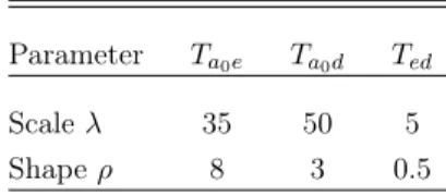
an illness or a group of illnesses which may cause the entry into a disability state, and state d represents the death state. When an insured is in state e, he has the possibility to report his claim (as defined by the insurance contract) after a certain time-lag. We assume that X is an homogeneous semi-Markov process where the failure times Ta0e, Ta0dand Ted are independent and follow Weibull
laws with parameters λ and ρ as defined in Table4. The set-up for the right censoring process C, the number of simulations and the sample size is exactly as in Section4.1.
Table 4: Simulation parameters used for the semi-Markov specification.
Parameter Ta0e Ta0d Ted
Scale λ 35 50 5 Shape ρ 8 3 0.5 Note: This table displays the simulation parameters used with Weibull distributions Wei pλ, ρq.
When an individual enters in state e, his health status is diagnosed and reported to the insurer after a random lag-time. It is unobserved until Tee1 where e1 corresponds to the disability state
triggering the payment of benefits in accordance with the contract. This latent time is simulated using a independent uniform distribution U rTa0e, Teds. From the insurer’s point of view, the
quan-tities of interest are the transition probability from a0 to e1 and not to e. With no loss of generality,
we consider the probabilities pa0e1ps, s ` 2q “ pa0e1ps, s ` 2, 0, r0, t ´ ssq “ P pXs`2 “ e
1
| Xs“ a0q
for s ě 0. Without right censoring, these quantities can be easily estimated not parametrically. Conversely, our estimators provide direct estimates of these quantities.
In this framework, let us consider now a second homogeneous semi-Markov model tX1
ptq , t ě 0u where X1ptq P ta
0, e1, dufor estimating the probabilities of interest on observable variables. The
du-ration laws for each transition are assumed to be Weibull Wei pν, σq where pν, σq are two parameters to estimate. Since the data are initially simulated using Weibull distributions and this law is quite flexible, one would expect a good quality in terms of goodness of fit. In particular, this approach fits well without the introduction of a latent period before the claim notification. Thus, we compute the transition probabilities by estimating first the transition intensities of the semi-Markov model and then by evaluating the following integral using numerical integration with a trapezoid rule and 1,000 samples P`Xs`2 “ e1| Xs“ a0 ˘ “ żs`2 s ¯ pa0a0ps, τ, 0q µa0e1pτ q ¯pe1e1pτ, t, 0q dτ .
The results of this comparison is presented in Table 5. Our estimators ppa0e1ps, s ` 2q and
q
pa0e1ps, s ` 2qoutperform the Markov estimators in terms of bias. Not surprisingly, the
semi-Markov estimators do show a smaller variance in many cases since the model is parametric. The superiority ofppa0e1ps, s ` 2qcompared to semi-Markov estimators is less clear as this estimator can
be seriously biased as noted in Section4.1.
5
Application to LTC insurance data
This Section describes our LTC insurance dataset and discusses the results obtained with our non-parametric estimators for transition probabilities. Here, we compare these estimators and measure
Table 5: Comparison with the estimated transition probabilities from state a0
to state e with a homogeneous semi-Markov model.
p
pa0e1ps, s ` 2q ppa0e1ps, s ` 2q qpa0e1ps, s ` 2q Semi-Markov model ps, tq n Censoring pa0e1ps, s ` 2q BIAS VAR MSE BIAS VAR MSE BIAS VAR MSE BIAS VAR MSE
(31.30,33.30) 100 Scenario 1 0.059 7.06 1.80 1.85 1.03 1.07 1.07 0.99 1.07 1.07 -19.55 0.42 0.80 (31.30,33.30) 100 Scenario 2 0.059 -1.42 1.57 1.57 -1.76 1.46 1.47 -1.79 1.46 1.46 -3.57 0.30 0.31 (31.30,33.30) 200 Scenario 1 0.059 6.70 0.88 0.93 0.22 0.53 0.53 0.21 0.53 0.53 -20.99 0.27 0.71 (31.30,33.30) 200 Scenario 2 0.059 0.72 0.78 0.78 0.70 0.70 0.70 0.72 0.70 0.70 -0.38 0.14 0.14 (31.30,33.30) 400 Scenario 1 0.059 6.25 0.51 0.55 0.12 0.27 0.27 0.13 0.27 0.27 -19.09 0.19 0.56 (31.30,33.30) 400 Scenario 2 0.059 -0.54 0.35 0.35 -0.44 0.33 0.33 -0.44 0.33 0.33 1.30 0.06 0.06 (35.16,37.16) 100 Scenario 1 0.112 25.79 6.20 6.86 -0.52 4.94 4.93 -0.48 4.88 4.87 -24.20 2.10 2.69 (35.16,37.16) 100 Scenario 2 0.112 -0.74 4.60 4.59 -0.92 4.23 4.23 -0.84 4.25 4.25 17.29 1.35 1.65 (35.16,37.16) 200 Scenario 1 0.112 20.85 4.19 4.62 -1.36 2.22 2.22 -1.27 2.21 2.21 -28.41 1.46 2.26 (35.16,37.16) 200 Scenario 2 0.112 0.34 2.31 2.30 0.02 2.13 2.12 0.07 2.12 2.12 27.32 0.56 1.30 (35.16,37.16) 400 Scenario 1 0.112 21.82 2.35 2.82 -1.16 1.13 1.13 -1.09 1.11 1.11 -23.18 1.24 1.78 (35.16,37.16) 400 Scenario 2 0.112 -0.77 1.16 1.16 -0.93 1.02 1.02 -0.96 1.02 1.02 32.38 0.22 1.27 (38.90,40.90) 100 Scenario 1 0.156 71.84 25.78 30.92 -4.21 24.34 24.33 ˚ ˚ ˚ -13.23 10.48 10.65 (38.90,40.90) 100 Scenario 2 0.156 -0.14 13.16 13.15 -2.15 11.70 11.70 -1.74 11.76 11.75 24.63 3.95 4.56 (38.90,40.90) 200 Scenario 1 0.156 68.03 16.13 20.74 2.59 10.36 10.36 ˚ ˚ ˚ -30.04 8.37 9.27 (38.90,40.90) 200 Scenario 2 0.156 -2.54 6.42 6.42 -3.79 6.06 6.07 -3.62 6.03 6.04 43.63 1.55 3.46 (38.90,40.90) 400 Scenario 1 0.156 62.88 9.42 13.37 -6.48 5.23 5.27 ˚ ˚ ˚ -20.33 8.34 8.74 (38.90,40.90) 400 Scenario 2 0.156 -4.90 3.30 3.32 -4.97 2.93 2.95 -4.99 2.92 2.94 53.11 0.56 3.38
Note: This table contains the estimates bias (BIAS) ˆ103, variance (VAR) ˆ103and mean square error (MSE) ˆ103with our non-parametric estimators. We compare the results at time s “ τ.20, s “ τ.40and s “ τ.60for samples with size n “ 100, n “ 200 and n “ 400. The results are obtained with K “ 1, 000 Monte
Carlo simulations. ˚ indicates that there is a lack of data for a particular time interval andqpa0e1ps, s ` 2q can not be estimated.
their uncertainty with a non-parametric bootstrap procedure.
5.1 Data description
The dataset that we analyze here is drawn from the database of a French LTC insurer. The corresponding policy offers fixed benefits for elderly people and covers the insured’s residual lifetime. The disability states only include the most severe degrees of disability and the contract does not allow to recover from a disability state. The insured pays his premium as long as he is in the healthy state. The guarantee is terminated or reduced after a fixed period of time when the policyholder stops paying the premium. Benefits may also be paid in case of death before entry in dependency or when the contract is reduced.
This dataset is almost the same as that used to estimate the probabilities of entry into depen-dency in Guibert and Planchet (2014). It is also studied by Tomas and Planchet (2013) with an adaptive non-parametric approach for smoothing the survival law of LTC claimants, but without distinguishing the effect of each disease causing the entry into dependency. In this last study, the authors compute the monthly death rates for the population of LTC heavy claimants and exhibit significant differences for duration times, indicating that the lifetime after entry into dependency clearly depends upon the age and the time elapsed since the entry. In addition, we have fitted a Cox semi-Markov model as a preliminary test to assess the Markov assumption, which returns the duration time as a significant factor. This means that the Markov assumption is not satisfied. Com-paring to these previous studies, we have improved the data by adding the individual cause-specific living path after entry into dependency.
The data are longitudinal with independent right-censoring and left-truncation. Most of the time, censoring occurs at the end of the observation period, but other administrative causes can
exist. For example, a policyholder may be censored if he refuses to continue paying his premiums and loses his rights. Left-truncation is induced by the entry date of a policyholder into the insurance portfolio. As the terms of the contract provide a lifetime coverage period, there is apparently no link between the truncation and the censoring times. For these reasons, the independence assumption for left-truncation and right censoring is considered to be satisfied.
The period of observation stretches from the beginning of 1998 to the end of 2010, and the range of ages is 65-90. Note that the definition of the disability states is relatively uniform over the studied period. We observe around 210,000 contracts and 68% of insured are censored before entering into dependency. The data are split into 4 groups of pathologies: neurological pathologies e1 (censoring rates=40%) including strokes, various pathologies e2 (censoring rates=36%), terminal
cancers e3 (censoring rates=6%) and dementia e4 (censoring rates=45%) including Alzheimer’s
disease. About 12,800 entries in dependency are observed. Considering death d1 and reduction
d2 as the other exit causes from the initial state, the multi-state structure of our dataset is shown
in Figure 4. The state d1 can be reached from all the disability states. We do not consider any
covariate in this application.
e1 a0 e4 d1 d2 .. . .. .
Figure 4: Multi-state structure of LTC data.
5.2 Estimation results for transition probabilities
Now, we perform the estimation of transition probabilities with each method presented in Section3, i.e. for e P te1, . . . , e4u: • Method 1: ppa0eps, t, 0, ∆vqand pped1ps, t, ∆u, 8q, • Method 2: pp ˚ a0eps, t, 0, ∆vqand pp ˚ ed1ps, t, ∆u, 8q, • Method 3: pq ˚ a0eps, t, 0, ∆vqand pq ˚ ed1ps, t, ∆u, 8q.
For brevity’s sake, we do not show the other transition probabilities of interest described in Section2, as studying (3.3) and (3.6) is sufficient to illustrate the methodological issue raised in this paper.
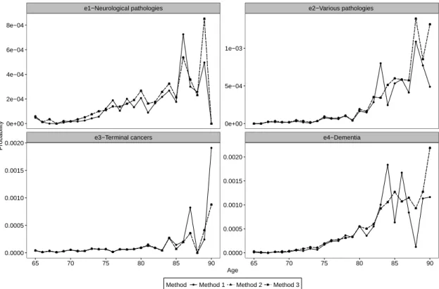
Figure 5 displays the estimates of the annual probabilities pa0eps, s ` 1, 0, ∆vq of becoming
dependent for an insured between the ages of s and s ` 1, and staying one month (∆v “ ‰0,121
‰ ) in a disability state6. Figure6 shows similarly the entry probabilities with a sojourn time between
five and six months, along the same range of ages. For each disease, transition probabilities globally
6
grow over time, with an acceleration after age 80. We note that the alternative estimators (Method 2 and Method 3) are virtually identical and are more robust than those calculated with Method 1. In most cases, the estimates related to Method 1 are smaller than its competitors, expect for some pics after the age of 80, suggesting than this method generates a negative bias here.
● ● ● ● ● ● ● ● ● ● ● ● ● ● ● ● ● ● ● ● ● ● ● ● ● ● ● ● ● ● ● ● ● ● ● ● ● ● ● ● ● ● ● ● ● ● ● ● ● ● ● ● ● ● ● ● ● ● ● ● ● ● ● ● ● ● ● ● ● ● ● ● ● ● ● ● ● ● ● ● ● ● ● ● ● ● ● ● ● ● ● ● ● ● ● ● ● ● ● ● ● ● ● ●
e1−Neurological pathologies e2−Various pathologies
e3−Terminal cancers e4−Dementia
0e+00 2e−04 4e−04 6e−04 8e−04 0e+00 5e−04 1e−03 0.0000 0.0005 0.0010 0.0015 0.0020 0.0000 0.0005 0.0010 0.0015 0.0020 65 70 75 80 85 90 65 70 75 80 85 90 Age Probability
Method ● Method 1 Method 2 Method 3
Figure 5: Annually estimated transition probabilities from the healthy state a0 to the dependency
states e1, . . . , e4 with Method 1, Method 2 and Method 3. The range of ages is 65-90 and the
sojourn time of one month.
Then, we analyze the estimated death probabilities from each disability state ped1ps, s ` 1{12, ∆u, 8q,
e “ e1, . . . , e4, on a monthly basis for each method. Monthly rates are computed since practitioners
are familiar with these quantities. As data are sparse for some time points, point estimates of transition probabilities may be erratic. For this reason, we choose to report a simple integrated version of these probabilities as follows
ped1ptsu, tsu ` 1{12, ∆u, 8q “
1{λ´1
ÿ
k“0
λped1ps ` kλ, s ` 1{12 ` kλ, ∆u, 8q,
for fixed values of s and ∆u, and with a monthly time step λ “ 1{12. This provides an average of
the monthly death probabilities for individuals entering in dependency with the same (integer) age. Note that a suitable choice for the weights and the calculation time points could be found, but we do not develop this point further to keep the comparison of methods as simple as possible. Figure7
and Figure 8 present these integrated transition probabilities for duration u varying between one month and six months, and with ages of occurrence equal to 75 and 80 respectively. We limit our analysis to these windows as censoring becomes important beyond a twelve months duration period for causes e1, e2 and e4, and observations are scarce for terminal cancers exceeding a period
of six months. We find that the residual lifetime (after an individual enters into dependency) is very different from one type of disease to another. In particular, the model shows extreme death
● ● ● ● ● ● ● ● ● ● ● ● ● ● ● ● ● ● ● ● ● ● ● ● ● ● ● ● ● ● ● ● ● ● ● ● ● ● ● ● ● ● ● ● ● ● ● ● ● ● ● ● ● ● ● ● ● ● ● ● ● ● ● ● ● ● ● ● ● ● ● ● ● ● ● ● ● ● ● ● ● ● ● ● ● ● ● ● ● ● ● ● ● ● ● ● ● ● ● ● ● ● ● ●
e1−Neurological pathologies e2−Various pathologies
e3−Terminal cancers e4−Dementia
0.0000 0.0004 0.0008 0.0012 0.000 0.001 0.002 0.003 0.00000 0.00025 0.00050 0.00075 0.00100 0.000 0.001 0.002 65 70 75 80 85 90 65 70 75 80 85 90 Age Probability
Method ● Method 1 Method 2 Method 3
Figure 6: Annually estimated transition probabilities from the healthy state a0 to the dependency
states e1, . . . , e4 with Method 1, Method 2 and Method 3. The range of ages is 65-90 and the
sojourn time between five and six months.
probabilities for terminal cancers for the first six months. The comparison between estimation methods provides interesting results. For causes e1, e2 and e4, both alternative estimators are quite
similar, with an exception for e2 at age 75 and for u “ 2. For terminal cancers, results given
by Method 3 seem to be underestimated, when the age of occurrence is 75. Conversely, results with Method 1 and Method 2 are close. Certainly, this is explained by a low censoring rate and a relatively small number of policyholders at this age. Additionally, estimates are close to each other at age 80, when increasing the exposure. This finding is comparable to results described in Section4
with Scenario 2.
We now report some point estimates for pa0eps, s, `1, 0, ∆vqin Table6and ped1ptsu, tsu ` 1{12, ∆u, 8q
in Table 7along with 95% confidence intervals at age s “ 75 and s “ 80. For that, the asymptotic variance is obtained with 500 bootstrap samples and the confidence intervals are deduced using the normal approximation. For both probabilities, the sojourn time in disability states are ∆v “ 1{12
and ∆v “ 1{2, and ∆u “ 1{12 and ∆u “ 1{2. We compare the results obtained with Method 1,
Method 2 and Method 3. In Table 6, results obtained with alternative estimators (Method 2 and Method 3) are virtually the same and are more robust than those of Method 1 in most cases, ex-cept for cause e2 at age 75. Estimates of ped1ptsu, tsu ` 1{12, ∆u, 8q are highly uncertain as the
amount of available data is insufficient. While remaining wary and critical due to this lack of relia-bility, we observe however that the difference between the two alternative estimators remains small, except for cause e3 for a duration of six months where data quality is probably poor. Ignoring
results for cause e3, note again that the 95% confidence intervals are generally larger for estimator
p