Acoustics in moving media

ACOUSTICS IN MOVING MEDIA

by

PETER GOTTLIEB

B.S., California Institute of Technology

(1956)

SUBMITTED IN PARTIAL FULFILLMENT OF

THE REQUIREMENTS FOR THE DEGREE OF

DOCTOR OF PHILOSOPHY

at the

MASSACHUSETTS INSTITUTE OF TECHNOLOGY

June 0959

Signature of Author

Department of Physics, 18 May 1959

Certified by

Thesi4 Supervisor Accepted by

Chairman,

Departmen"Kmittee on Graduate Students

0' - - , ." , I . 1 11 = I

AUG 10 1959

ACOUSTICS IN MOVING MEDIA

Peter Gottlieb

Submitted to the Department of Physics on 18 May 1959 in partial

ful-fillment of the requirements for the degree of Doctor of Philosophy.

ABSTRACT

This thesis is concerned with two types of problems

in-volving moving fluids and sound.

The first problem is to determine

the qualitative conditions necessary for instability due to infinitesimal

acoustic disturbances.

The particular technique used here is to

as-sume that the disturbances are fixed in space while the fluid flows

past them.

This viewpoint is applied to the questions of turbulence

onset and resonator excitation.

The second problem is to examine some of the

quantita-tive properties of an interface between two media in relaquantita-tive motion.

In particular, the sound field due to a source near such an interface

is calculated.

It is shown that the sound field can be approximated

in a closed form by a saddle point integration, and this will be a valid

approximation for distances from the source which are large as

com-pared to the wave length of the emitted sound.

This situation is

gen-eralized to the study of the characteristics of a channel formed by

two parallel velocity discontinuity interfaces.

Then, it is further

generalized to include the possibility of a plate or membrane along

the interface separating the two media in relative motion.

The

sta-bility of the interface is discussed as each of the various cases arises.

Thesis Supervisor:

Uno Ingard

7

ACKNOWLEDGMENTS

The author wishes to thank Professor Uno Ingard for the

suggestions and conversations which led to the formulation of this work

and for his comments and encouragement during the course of the

cal-culations.

Also, it is a pleasure to have this opportunity to thank

Professor Philip M. Morse and Professor Herman Feshbach for

read-ing the manuscript and suggestread-ing a number of improvements.

Finally, the author wishes to express his appreciation to

both the Office of Naval Research and the Owens-Corning Fiberglas

Corporation whose support has made this work possible.

TABLE OF CONTENTS

Page

Abstract ...

Acknowledgments ... List of Figures... . .. . . Introduction ...

CHAPTER 1-Wave Equation and Instabilities ...

I.

Derivation of Wave Equation in Moving Media ....

II.

Instability due to Inhomogeneous Terms ...

III. Solution of Wave Equation for Channels ... IV. Resonator Excitation...

CHAPTER 2-General Discussion of a Tangential Velocity Dis-continuity ...

I. Boundary Conditions for the Reflection and Refraction of Sound ...

II. Helmholz Instability ...

III. Transmission through Many Layers ... CHAPTER 3- Line Source ...

I. Formal Integral Solutions ...

II.

III.

IV.

V.

CHAPTER

14 14 18 18 23 23 25 37 40 43 50

50

51

Evaluation of Integral for Transmitted Wave ...

Evaluation of Integral for Reflected Waves ...

Modification Necessary for the Supersonic Case .

Some Additional Terms for the Near Field ...

4- Point Source...

I. Formal Integral Solutions ...

II. Evaluation of Integrals for Transmitted Wave....

ii

iii

vi

viii

1

1

3

6

9

-"- _1290sompow- 1, .1, 0 -- - - __ __ t 0!114, - -==a

Page

CHAPTER 5-Line Source in a Velocity Discontinuity Channel..

60

I.

Formal Integral Solutions... ...

60

II.

Discussion of Characteristic Equation... ...

63

III.

Evaluation of Integrals ...

...

69

IV.

Cylindrical Channel...

70

CHAPTER 6-Flow Discontinuity with Plate or Membrane

Separation ...

75

I.

Formal Integral Solutions

...

75

II.

Discussion of Characteristic Equation

...

78

III.

Evaluation of Transmitted Field...

84

Summary and Conclusion ...

91

Bibliography...

93

Biography...

95

LIST OF FIGURES

Figure

Page

1.

Flow Past a Closed Pipe

Resonator...

10

2.

Experimental and Theoretical Curves of Neutral Stability

for a Closed Pipe Resonator

...

12

3.

A Velocity Discontinuity with Incident, Reflected, and

Transmitted Sound Waves...

15

4.

Flow with Constant Gradient Broken into Layers of

Constant Velocity...

19

5.

Sound Source near a Velocity Discontinuity ...

24

6.

The Path of Integration in the k Plane ...

27

7.

Branch Points of the Integrand for

, or . ...

28

8.

A Plot of Eq. (3.7) for Constant r with M

=

3 ...

31

9.

The Same as Fig. 8 withM

1 =

1.? ...

32

10.

A Plot of Eq. (3.9) for Constant R with M

=

3 ...

34

11.

A Plot of Eq. (3.9) for Constant R with M2

=

.7

...

35

12.

A Plot of Eq. (3.9) for Constant R with M

2 =

1.2 ...

36

13.

A Plot of Eq. (3.1 2) for Constant R with M

=

5...

..*..

39

14.

Saddle Path for M > 1

with Branch Cut at Mach Angle.

42

15.

Saddle Path for 42 and Cut for 4 ...

44

16.

The Cut and Saddle Path for Medium 2 with M,

< 1

and

M2

>'1''..''..'...'

...

45

17.

The Range of Values of

X0

and the Locus of Branch

Points for Y, = 0... 54

Figure

Page

18.

Saddle Path, Branch Points, and Branch Cut for the

p Integration...

56

19.

Channel Formed by two Velocity Discontinuities ...

..

61

20.

Lowest Mode Characteristic Given by Eq. (5.9a) ...

..

64

21.

Lowest Mode Characteristics Given by Eq. (5.9b) ...

65

22.

Illustration of the Geometrical Conditions Necessary for

a Propagating

Mode...

66

23.

Cut-off Frequencies for the Lowest Few Modes of the

Two-Dimensional Channel ...

68

24.

Cylindrically Symetric Velocity Discontinuity Channel or

Jet...

71

25.

Poles, Branch Points, and the Saddle Path for the

Integration of Eq. (6.2) or Eq. (6.3)...

83

INTRODUCTION

The main problem to be discussed here is the determination

of the far field sound due to point and line sources in moving media near

various types of velocity discontinuities.

The main motivation for this

research is the study of jet noise.

The sound sources are inside the jet,

and it is most practical to make the measurements outside the jet. Thus,

it is necessary to know the effect of the jet boundary on the directionality

of the source.

If this boundary is idealized to a sharp velocity

discontin-uity, then the far field can be calculated.

A comparison of the

experi-mental and theoretical results is found in the conclusion at the end of this

thesis.

This problem of valocity discontinuities raises the question of

stability, which, properly, should (and will) be taken up first. As an

in-troduction to the valocity discontinuity instability, it is interesting to

ex-amine a few well-known examples of instability from a unified physical

point of view.

The particular examples of turbulence onset and resonator

excitation are discussed in Chapter 1,

and the remainder of the thesis is

devoted to the velocity discontinuities mentioned above.

The turbulence problem has been treated in detail by a

num-ber of authors,

but K. Schuster(

2

) has recently suggested a different

particular, this concept leads to a natural explanation of some recent

data(3) on resonator excitation by steady flow.

A discussion of the

va-lidity and possible extension of this concept is presented in the conclusion.

WAVE EQUATION AND INSTABILITIES

I.

Derivation of Wave Equation in Moving Media

The wave equation for sound in a nonuniform moving medium

has been derived in many places, so it would hardly seem necessary to

give another derivation here.

However, there are two reasons for

reviv-ing old memories at this time.

In the first place, the wave equation is

the basis for all of the work presented in this thesis.

The other reason

is that it is interesting to see how some of the terms which cause

instabil-ity arise.

We start with the Navier

-

Stokes equation for a compressible

fluid, neglecting viscosity (for the time being) and heat conduction, and

considering the sound to be isentropic.

(ai/at)

+

(iii

- 1

)di

P/P

(where u is the total velocity vector).

In addition, we must use the

con-tinuity equation

(ap/at)

+ V

(p-u)

=

0.

The usual procedure is to eliminate the linear terms in

u.

This gives

The pressure can be expressed in terms of the density (or vice versa) to

any desired degree of accuracy, but it is still difficult to disentangle the

nonlinear term on the right-hand side of Eq. (1.1).

One procedure is to

divide the total velocity into the steady flow V and the fluctuating, or

sound, velocity V.

Then, the wave equation is linearized in the sound

variables.

One example of frequently encountered steady velocity

distri-bution is a two-dimensional flow with the velocity vector along the x-axis

and the magnitude of the velocity depending only upon y.

This is the case

for flow in channels and many similar situations.

Since the steady flow

is incompressible, p and p are constant except for sound fluctuations.

2

Thus, to first order in acoustic variables, p

=

c p,

and the left-hand

side of Eq. (1.1) becomes a scalar wave equation.

If V

<<

c, the

right-hand side of Eq. (1.1) can be treated as a perturbation, and the scalar

wave solutions can be substituted in it to get

POV-0

2

v x/8x

2

)

+

p

0

V(

2

v

/8xay)

+ p

0

(aV/ay)

(8vy/ax)

(l.la)

for the perturbing terms.

All of the terms in V

2

have been omitted since

they are of higher order in this approximation.

We return to them later

when considering higher-order approximations and homogeneous flow

dis-tributions.

The question of stability of steady flows can be considered as

the question of growth of small disturbances.

With this concept in mind,

we can consider the terms of (1.la) as driving terms for the scalar wave

damp-~~~~~~'1 -~

ing.

But a phenomenological damping term can always be introduced.

Then, the sound wave will grow exponentially (and the flow will be

un-stable) whenever the driving terms are larger than the damping term.

In addition, it is necessary for the driving terms to be in phase with the

damping term.

II.

Instability due to Inhomogeneous Terms

To clarify this reasoning with an example, we consider

or-dinary parabolic flow in a two-dimensional channel.

In keeping with the

above restriction of flow in the x-direction varying in the y-direction,

the width of the channel is taken from y = - (d/2) to y =

(d/2).

Then,

the steady flow can be written as

V = V0

(1

-

4y

/d2

).

Considering the fundamental mode of the channel as a wave guide, the

sound variables can be written as

p = Asink y i(t - kxx)

In y

k 2+

kx +k0

k

(

2=

/c2

2

vx

=

[ Ak sin kyyei(ot - kxx)]

/0

=

0

+

a

v = - [Ak cos k y ei(t - kxx)] ip0O k = Tr/d

y

y

y

y

p = (A/ c2) sink y yei(wt - kxx)

(1.2)

driving (perturbation) terms.

Equation (1.1) can be written as [using

the terms of (1.1a) for the right-hand side and using the damping term

R(ap/at)]

(02p/at2) + R(Op/Ot) - c 2 2

p

0

V(2v /ax2

+ P0

V

2v/axay) +

y

2

(If the viscosity had been included in Eq. (1.1), we would have R

= -

V

as is explained later. ) With the substitution of all of the appropriate

pre-viously defined quantities, this becomes

[- (2wa /c ) + _{(iwR/c 2)] sin kyy = (k xV 0}

_/c2

₁

_-

_(4Y2/d2)]

_sin

_kyy

-(8k k y/d2) cos k y . (1.3)

x

y

y

[ That we are not concerned that the -terms of (1.3) do not have the same

y dependence is shown later. ]

It is now apparent why the perturbation

terms on the right-hand side of (1.3) must have the same phase as the

damping term in order to produce instability.

This will cause a to be

imaginary, and, if the perturbation terms are larger than the damping

term, a will be negative imaginary which gives an exponential increasing

in time.

Of course, this derivation has been sloppy, and all of the terms

in Eq. (1.3) do not have the same dependence on y, so the equation

im-plies that the perturbation excites higher modes.

At this point, the most

convenient procedure is to make the approximation that both sides have

the same y dependence.

Once y is eliminated, we can take the usual

lumped parameter form for R

=

w/Q.

Then, we can obtain a crude

ap-proximation from Eq. (1.3):

- 2wa

C/c

2 _ _ 2

/c

2

Q)

+

(V

k W/c

(1.4)

The approximation used thus far may seem outrageous, but it is shown later that there is a sufficiently rigorous, but intuitively obscure, method for obtaining a remarkably similar result. At the present point, it must be noted that k must be imaginary to produce instability. This means

that the mode is below cut off for the guide. If we make the substitutions

E = Wd/wc; M = Vo/c; and y = kinematic viscosity with Q = 3/2rE and r = lTy/cd for damping due to viscosity, then, for the onset of in-stability, a = 0 in Eq. (1.4), which gives

M/r = 2E 2/3f-7 2 = R

/2i

(1.5)

(where R? is the critical Reynolds number with a sound wave, of frequen-

_k

cy given by E, below cut off). If the channel is considered as a resonator (standing wave across the width), R can be averaged over that pert of the frequency spectrum which has E -< 1 (or frequency below cut off) to obtain the critical Reynolds number for the flow

Rk=

R t4 (,e) de = (41T/3) NF_ O

(Q

0 = 3/2r) (1.6)

In keeping with the crudeness of this derivation, the frequency distribution has been approximated by

4(E) = QO for 1- (2/Q 0)<E <1

The above result agrees reasonably well with experiment.

The method is similar to that used by K. Schuster(2)

and the

compari-son with experimental results is given in his paper.

After Eq. (1.4),

the present treatment is identical with that of Schuster, but the

deriva-tion of Eq. (1.4) is rather novel in its direct approach showing the

par-ticular terms in the wave equation which are responsible for the

amplifi-cation and instability.

III.

Solution of Wave Equation for Channels

The derivation of Eq. (1.4) by Schuster is more rigorous than

is mine, but it is possible to give a much more rigorous treatment than

Schuster did by solving the wave equation for parabolic steady flow.

For

this treatment, the y dependence of p is left unspecified, and the density

fluctuation is taken to be of the form

p =

Fy) ei(wt - kxx)

p

=

F(y) ei(tkx

(1.7)

Now, the two components of the Navier

-

Stokes equation can be written as

(avx/at) + V(avx/8x) + v (aV/ay) = -

(c

2

/p)

ax)

y

(Ov /at)

+

V(av /ax)

= -

(c

2

/p

0

)

(ap/8y)

,

(1.8a)

y

y

and the continuity equation can be written as

~Im~

Since v

and vy must have the same form as p ['given in Eq.

(1.7)],

they can be eliminated from Eq. (1.8a) and Eq. (1.8b) to give

(8 2F/y2) + (2k (2V/ay) (8F/ay))/(w - k V)] + [(o - k V)2 (1/c2

2

k ] F = 0.

In order to solve this equation, we must make the approximation o >> k V.

x

Then, using the explicit V(y),

FN - (6k V0/od2) yF + [2 /c2)

Eq. (1. 9a) becomes

2 (2ck

V

/c

2

)

+ (8wok V0y2

c

2d 2)]F = 0

(where the prime denotes differentiation with respect to y). If the first derivative term is removed by the substitution

F = (y) e(4kxV0

/od

2)y2

then Eq. (1.9b) becomes

4i' +[(W2/c) - k 2 (2wk V /c2 x xO0 + (8k V0/od 2_{) + (8k V} 0Z2/d2) (( 2/c 2

)

(1.10) (8kVx V 0/c 2d2)) = 0

This can be put in a standard form by the substitution

= K 1 _y

which gives,

(d2 /d 2) + K = - (32k V0/d2)

[

2/c2) + (8k V /W2d2) in place of Eq. (1.10) K

/1/412

- k2

_x

- (2ok V₀/c2) + (8k V0

/od

2

-

2 /4)]4 = 0. (I.IOa)

(1.9a)

(1.9b) + - k

- _____---.--- -. - - -~

This equation is the same as the Schroedinger equation for the harmonic oscillator, and the solutions 4 are called parabolic cylinder functions or Weber - Hermite functions. The eigen values which satisfy the boundary conditions

(80/ a)= 0 at = +_ (rd/2)

have been approximated by F. C. Auluck 4 ) for the lowest few orders in the parameter k V/W. If W = W0 + a + iw/Q, then the eigen value equa-tion is

- (2wa

/c2)

_(ic /Qc2) + (k V

/W) [

(W 2/c )(4/3 + 4/T) - 8/d2] This is seen to be similar to Eq. (1.4), except that the amplifying term will only have the proper sign if

E > 2/(1 + Tr2/3)

Since only values of E close to 1 were used in the calculation of critical Reynolds number, the instability calculation is still valid, and the intuitive approach leading to Eq. (1.4) is seen to give fairly accurate results.

It should be noted that the treatment of Sections II and III differs radically from the conventional stability analysis, as has been mentioned in the Introduction. Usually, the stability of the propagating modes of the channel is examined. The present discussion considered only the nonprop-agating mode stability.

)

IV. Resonator Excitation

The instability of nonpropagating disturbances leads to the instability of systems like resonators which create stationary disturbances while a fluid flows past them. Such a situation for a closed pipe resonator is shown in Fig. 1. The fluid has a constant velocity in the x direction as shown, and, for resonance, there is a standing wave, with variation along the y-axis, in the resonator. Since the velocity is constant in the moving fluid, the wave equation (including viscosity) can be written quite simply as

(82p/t2) _

(p/Ot)

- c2 (8 p/y2) = c2 ( /

)

- 2V(8p/8xot)

-V2

(a

2

_p/ax

₂ 2

_(/8)

_(1.12)

As shown in Fig. 1, the moving fluid moves a short distance into the mouth of the pipe; beyond that, there is no x variation in the pipe for the funda-mental mode, so all terms on the right-hand side of Eq. (1.12) are zero. Furthermore, the LLeft-hand side of Eq. (1.12) can be written in lumped parameter form as a resonator equation, and set equal to sero for the low-est order solution,

(8

2p/8t

)

+

(o

0

/Q)

(ap/at)

+

W

=

0

(1.13)

(where w0 = ctr/2d for the pipe fundamental). The value of Q is found

from the viscous and radiation damping, but left unspecified for the moment. The solutions satisfying E2. (1.13) are of the form

pI =

(p0 A

1

/c)sin(rry/2d)

(sinw0t +

-coso

0t) . (1.14)

x

2-Figure

1.

FLOW PAST A CLOSED PIPE RESONATOR

10

F

V

We next consider the terms on the right-hand side of Eq. (1.12) in the moving fluid (in particular, that part of the fluid which extends

slightly into the resonator, as shown in Fig. 1). These terms can cause instability if they have the same time phase as the damping term on the left of Eq. (1.12). We find their phase just inside the resonator mouth by using the p1 time dependence from Eq. (1.14). The first term on the

right-hand side of (1.12) is not of interest, since it is not multiplied by the velocity, and so does not contribute to the excitation. The next term

2

2

2

V(82p/8x8t) has the required time phase. The term V (82p/ax ) has the reactive time phase for the large term of p1. (This merely produces the

well-known frequency shift.) The small term of p1 gives the damping

phase for this term. The last term is a viscosity term which has the re-active time phase for the large term of p1, and the damping time

depen-dence for the small term. If the viscous effects are small, this term can be neglected. The terms of interest are now the second and the small part of the third term on the right-hand side of Eq. (1.12). To put these terms in a lumped parameter form such as Eq. (1.13) would require a knowledge of the exact wave field over the interaction volume. Therefore, it is most convenient to leave the parameters of these terms unspecified, except for sign. A look at Fig. 1 reveals that the interaction volume will be greatest on the x > 0 side of the pipe (where the moving fluid comes the furthest into the pipe). At this side, (p/ax) e' - (p/1), since the field is expected to be a maximum at the center and fall off for large x.

Thus, Eq. (1.12) becomes (considering only terms with damping time phase)

Q

EXPERIMENTAL--THEORETICAL

V

Figure 2. EXPERIMENTAL AND THEORETICAL CURVES OF NEUTRAL

STABILITY FOR A CLOSED PIPE RESONATOR

(The minimum is at

i

=1.)

21w

0

12

(where g and h are unspecified positive parameters).

Just as in the previous example, it is the disturbance which is exponentially damped in space which causes the unstable, exponentially increasing disturbance in time. In Fig. 2, Q is plotted as a function of V, with g and h adjusted to make the minimum of the theoretical and ex-perimental curves coincide. The experimental data are due to L. W. Dean.(3)

GENERAL DISCUSSION OF A TANGENTIAL VELOCITY DISCONTINUITY

I. Boundary Conditions for the Reflection and Refraction of Sound

The remainder of this thesis is devoted to fluids with constant velocity in each of two regions, but with a different velocity in each region. In addition, the boundary between the two regions will be taken parallel to the flow direction, which is taken to be the same in the two regions. The problem of reflection and refraction of a plane sound wave from such an

in-(5)

(6)

terface has been considered recently in papers by Miles and by Ribner, but it is of interest to repeat the derivation here in a slightly different manner.

The geometry is pictured in Fig. 3. Medium 1 is at rest, and medium 2 is identical with medium 1 in all properties (for the sake of sim-plicity) but has velocity V in the positive y direction as shown. In medium

1, the solution of the wave equation for the acoustic velocity potential can be written quite simply. For the wave incident at the angle as shown,

0=

e

t - iky -

yx

_ eiCt - (iW/c)(y cos 1 + x sinO)

(2.1)

(withy 1 = Jk-

(

2/c2) , k = (w/cw)cosO .

By the same reasoning, the reflected wave can be written as

xI TRANSMITTED

V

2

Ga INCIDENT WAVE

REFLECTED

WAVE

A VELOCITY DISCONTINUITY WITH INCIDENT, REFLECTED, AND TRANSMITTED SOUND WAVES

15

WAVE

y

Figure 3.

---A must be determined fuom the boundary conditions at x = 0.

Thus far, the coordinate system has been considered at rest relative to medium 1. If the coordinate system is transformed to mo-tion with velocity V, then, the potential in medium 2 can be written just as simply as Eq. (2.1). Then, the transmitted wave with frequency W2 can be written as

2 = Be1o2t - (iW2

/

c)y2 cos 02 - (iw2/ c) x2 sin 02 (2.3)

(with 0., x2, y2 being coordinates at rest with respect to medium 2,

x2 ~x y2 = y - Vt). Since all values of y and t must give the same phase for "1 and 02 at the boundary x = 0,

W = 2 (1 + M Cos 02) (coefficient of t)

Wcos0 = W2 cos 02 (coefficient of y) (2.4)

(where M = V/c). These equations were first given by Rayleigh(7) to determine the angle of refraction as a function of incidence angle. Using the relations of Eq. (2.4), it is evident that

k

₂ may be written as

2= Bi -ytY2x (2.5)

22

[Y 2 =k 2 - ( 2 /c2) W 2 = o-kV]

This is the form most convenient for the application of the boundary con-ditions.

p=

P

(0/at),

but in a moving medium

p =

p(ao4/8t)

+ pV(aO/ay),

from the linearized Bernouli equation.

Thus, the continuity of pressure

boundary condition is

w(O+ 01) = w20

(2.6)

If we call the boundary displacement ! in the coordinate system at rest,

then the velocity of the boundary in a coordinate system fixed to medium

2 is (ar/8t)

+

V (8/8y).

Now, 11 must have the same exponent as 00

0 , 02 for x

=

0, and the x component of velocity in medium 2 is

given by 8t2/ax, so the definition of r gives

i(w - kV)r _{-j 2}

iWr1

=Y

y(40

₁ -0

We can eliminate il from these equations to obtain the second boundary

equation

(-Y

/

w) 0 1

2/Z

2 (2.7)

Now, Eqs. (2.6) and (2.7) may be solved simultaneously to give

2

2

2

2

A = (y₁& ₂ - 'Y2'

)/(y

Y_{1 2} + y₂w

)

and

=(2

w )/(Y_{1 2} 2 2 (2.8)

II.

Helmholz Instability

If the denominator in Eq. (2.8) becomes zero, we have the well-known Helmholz instability. This denominator can be factored to

(k2 - yly ₂)( ₁ + y2), so that the Helmholz instability is given by

2

k = y 2'

The roots of this equation are

(kc)/

=[(M/2)

+ i 1 + M2 -

1

-

(M/4) ]

/

[

1

+ M - 1]

(2.9)

These will be complex for M < 2N12, which means that the interface is unstable. This instability has been discussed by a number of writers, and the most recent and most thorough discussion was given by J. Miles. He showed that the complex frequency given by Eq. (2.9), with the ima-ginary part both positive and negative, causes an initial disturbance of the interface to grow exponentially, in time. This leads one to question the meaning of the reflection and transmission coefficients calculated above. However, we can get physically sensible results by ignoring the poles entirely. This is shown in the next section. The effect upon the Helmholz instability, of a plate or membrane separating medium 1 and medium 2, is discussed in Section II of Chapter 6.

III. Transmission through Many Layers

It is interesting to use Eq. (2.8) in an experimentally known situation, and to check the results by an analytic calculation. One

possi-Vn

V

₂

VI

9

9

MULTIPLE REFLECTIONS

INCIDENT

WAVE

REFLECTED

WAVE

Figure

4.

FLOW WITH CONSTANT GRADIENT BROKEN INTO LAYERS

OF CONSTANT VELOCITY

19

bility is shown in Fig. 4. For x > 0, the fluid has a velocity in the positive y direction given by M = bx (with b constant). If we have nearly normal incidence (cos 0 < 1), and, if M < 1 for the region under consideration, we can take a plane wave solution of the form

p = e iot - (iW cos 0/ c)F(x), _(2.10)

and cos 0 will be approximately constant. The wave equation becomes (neglecting terms of order M2 cos2 0)

(d2F/dx2) + 2b cos 0 (dF/dx) + (w2 /c

)

(sin 2 - 2bx cos 0) F = 0. (2.11)

The exact solution of Eq.

F (x) =

NUl1/2 Z1/ 2 U3/2 ) e- bx cos 6 1/3 3

[ where N is a normalizing factor,

(2.11) is well-known as

is an appropriate Bessel or Hankel function of 113 order, and where

U = (sin20 - 2bx cos

0)/[

(2bc cos

0)/w

]2/3]

Now, if the approximation cos 0 << 1 is made again, form of the Hankel function may be used to obtain

the asymptotic

H1

/3

2 [ (2/3)u3f2]

If the pressure is given at x = 0 and a specified value of 0, then the normalizing factors are determined, and Eq. (2.10) becomes

p(x, O)/p(0, 0) -

[1

- (Mcos 0/2)] et - (ioycos

/c)

- (iwx/c) (2.12)

Now, Eq. (2.8) can be applied to this same problem. First, the continuous flow distribution must be broken into layers of constant velocity, as shown in Fig. 4. Then the sound field in layer n is found by taking the product of all of the transmission coefficients for the inter-faces between the layers preceding n. With the use of B from Eq. (2.8), the pressure transmission coefficient at an interface can be written, to first approximation in M co s 0, as

pl/po 1 - (MicosO/2) (2.13)

Now, we cannot match solutions at the interfaces in Fig. 4 in the manner used for the interface of Fig. 3 to derive Eq. (2.8). This is because there must be waves travelling in both x directions for each layer. In other words, the amplitude in the second layer is not found simply from the product of the transmission coefficients of the first and second layers, but must also be found from the transmission coefficients after each of the multiple reflections shown in Fig. 4. However, since M cos 0 << 1 throughout the region under consideration, it is seen that the reflection coefficient at the n- layer is of the order of magnitude M ncos 0. Since any fraction of the wave which is reflected once must be reflected a second time before it can contribute to the transmitted fraction, the con-tribution, to the transmitted wave, due to multiple reflections will be of

2

order of magnitude (M cos 0) . Since the present approximation is only to the order Mcos 0, these multiple reflections can be neglected entirely, and the amplitude can be calculated from the product of transmission co-efficients, as was suggested to begin with. To the same approximation as

Eq. (2.13), the transmission coefficient from the (n - 1) to the n layer can be written as

(Pn n -

I)

-~

1

- [ (Mn - M 1

)

cos 0/2],

and the product of the transmission coefficients up to the n--h layer can be approximated by

(pn ) ~ 1 - (Mncoso/2) . (2. 14)

This is seen to agree with the amplitude factor in Eq. (2.12), so the two different methods give the same result.

In physical situations, viscosity makes a flow like that shown in Fig. 4 stable, for low enough Reynolds numbers. Thus, the results of Section I have physical meaning, in spite of the Helmholz instability. In most of the following, we neglect this instability entirely.

LINE SOURCE

I. Formal Integral Solutions

The geometrical situation for a line source located near a velocity discontinuity is shown in Fig. 5. The coordinate system is fixed with respect to the source and the two media have Mach numbers M1 =

(V,/c), M2 = (V2/c) with respect to this fixed system. The plane wave expansion of a line source in a medium with velocity V1 relative to a

coordinate system fixed in that source is

i.t +OO

0 e [eiky-yx+hi

/y]dk

(3.1)

[where y₁ = Vk 2l - M1

)

- (W

/c

)

+ (2kM

c/c)

].

The total field will be made up of

40

plus the reflected wave in medium 1. In medium 2, the field will be simply the transmitted wave. The reflected wave can be written as

=ieLt A(k) e-iky+ ylx dk. (3.2)

And the transmitted wave is

4 MEDIUM 2 V2 y h 'SOURCE MEDIUM 1

SOUND SOURCE NEAR A VELOCITY DISCONTINUITY

24

V

₁

Figure 5.

[(with y= k21 M2 ) - (W 2/c

)

+ (2kM2o/c)

].

If we make the simplification of notation

= -

kMIc

W2 = W - kM2c

then, the continuity of pressure boundary condition becomes

( ₁ e Ylh/y) + ,,A = 2B,

and the continuity of the velocity normal to the interface gives

- (eY 1

/wj)

+ (yA/a) = -

(y

2B/ 2

).

Solving the boundary equations for A and B gives

2 2 2 2 -ylh

A = (,y 2 -yj 2 ) Yi(1 w2 + Y2w] e

B = [2w W2A 1 2 + y2 2IeY1h

This result is seen to be similar to Eq. (2.8), and the derivation leading to it is also similar to the derivation of Eq. (2.8).

II. Evaluation of Integral for Transmitted Wave

The next step is to evaluate the integrals of (3.21 and (3.3). The integral for 02 can be written as

+00

T0

g(k) ef(k) dk

-00

Since this integral is incapable of an exact analytic evaluation, the natural thing is to try the asymptotic approximation for the far field. For the saddle point method,

f(k) =

f(k

₀

)

+ (k - k0) ft(k0

)

+ [ (k - k0

)

2

/2]

fU(k).

And we solve for k0 given by ft(k0 ) = 0. If we substitute x = r sin 0, y =

rcosO,

k= [w/c(l - Mf)] [- M2 + (cos 0/41 - Msin20)]

(3.5)

(where the positive square root is always understood). It is noted that k0 has a branch point at 0 = -r/2, and the proper branch is chosen as the positive sign to satisfy the subsonic radiation conditions for y

>>

c/w. We can then calculate

f0(k = -i(c/w)[(l - M 2 sin 20)3/sin20] r

0

2

The path of integration must be chosen so that the phase of (k - k0) is

i. The two possible paths are shown in Fig. 6. The appropriate path goes in the positive real k direction, since the integral is over real values of k from -oo to +o. We must be careful about crossing branch points of the integrand. (Poles are neglected entirely in this analysis, as was suggested in Section II, Chapter 2. ) If we assume an infinitesimal amount of damping, the branch points are as shown in Fig. 7. When the saddle point is to the left of -(W c), we will have to cross the -(I/c)branch point in order to distort the real axis path into the saddle path. Thus, the

Im(k)

______________/4

Re (k)

THE PHASE REQUIREMENT /

FOR THE SADDLE PATH IS

SATISFIED BY THE 2

DIRECTIONS ALONG THIS

BROKEN LINE.

Figure 6. THE PATH OF INTEGRATION IN THE k PLANE (The path of integration is originally along the real axis,

but in the neighborhood of the saddle point it is distorted so that it crosses the real axis at the saddle point, making an angle of 45 with the real axis.)

EXTENSION OF RANGE

FOR MEDIUM 2 SADDLE

POINT FOR

M2>

1

RANGE OF MEDIUM 1

SADDLE POINT

Im(k)

RANGE OF MEDIUM 2

SADDLE POINT

Re(k)

EXTENSION OF RANGE

OF MEDIUM 1 SADDLE

POINT FOR

M

>l

S-x

/(V

-c )

KW/(V2+c)

Figure 7. BRANCH POINTS OF 'THE INTEGRAND FOR OR (FOR ( INSIDE THE MACH ANGLE)

I

L&xl) ( V2

sound field will have an extra term coming from an integration over a

cut surrounding the -(wl/c) branch point.

(This is explained in detail

in Section V of this chapter.)

This will be found to correspond to the

Vrefraction arrivalm (also explained in Section V), and will have a

straight wave fron: with a fall off of r-3/2 so that it makes no

contribu-tion to the far field.

The integral of Eq. (3.4) can now be approximated

by the integration over the saddle point to give

f (k )+ ist

2= s[(2rr/f"(k

0

)] g (k

0

) e~ f

+(3.6)

h, 2 2 with g(k) = [2 1

(2 e

2 2 =

isin0/N - M sin 0

I

2

-

22

2

2

2

cy2/o

=

[(-

M

1)/(1- M2 ) 2 [M 2 - (2M 2cos

O/

1 - 2 sin 2) +

2

2

2

(cos

0/[

- 2 sin

0])

3

-

1

- (2MM ₂

/[

-

2

+

[

2Mcos

/

2

2

2

~

1/2

(-M

2

)

1

- Msin2

/

Note: In most of the remaining work, we use the terminology

A

= (1 -

M

2 2

)1

It should be noted that y

is real for k

0

to the left of -(w,/c) in Fig. 7.

This means that all waves in this region are reduced by a factor e~Ylh

The physical reason for this is that for the Bleast time! path

k

0

>

is rather complicated, but two

cases

permit straightforward

interpreta-tion.

First, consider M

=

0.

2

=

[Zeit+(ir/4)

- hcosZ -(1-M cos)2 - (i/c)ycosO - (ifc)x sin

(I -

Micos

)

(isinO

+

cosO

- (1 -

M

cosO)2

/(

- McosO)

\ro/r

.

(3.7)

This equation is plotted in Figs. 8 and 9 for constant r. The factor

multi-plying h in the exponential is real for cos

0

> 1/(l

+

Mi)] which gives

the Ozone of silences at cos

0 =

(l/(l ± M

1

)] and 02 has a maximum.

However, the saddle point integration is a poor approximation in the

neigh-borhood of this point, since it is here that yj(k

0

)

=

0 (branch point).

This expression is valid for all values of Mi.

Equation (3.7) is the

lead-1/2

ing term of the far field approximation, so the r~

dependence is as

ex-pected.

The next order terms have an r3/2 dependence.

In all of these

cases, we have assumed r >> h, c/o.

The other straightforward situation is for M

=

0.

In this

case,

=

[Z'A3

-

MAsin0) e

it -(ir/4)-

hNf

(A cos-M)

/(-M

-[2iy/(l-M

2

_{MA sinco)}

_)/

[y/(

-M

)A

cos 0 - M) -ixA

sin 0

(1 -M2)

Asin0+

I - MA Cos 0)/

(1- M)2

2

1

-

M-A cos 0)/(1

-

M

2

)

NFrJ

c

)

(3.8)

330 n4 3*W 33W \ I 34100 30 x ! aA

/X

1IV Z\ Z

coka

the

e ~

~

pp

ag -fth

~

~

n

731

20' 3501 I 01 . .... . . . .. ... 320 310*' 100 700 'of0 240* 120* 6>4*0 10*

330*

00

30~ 10' 2

~0~

301000 30 SO: 4;' 240' 1230'

w

omitted. ) This rather forbidding expression can be simplified by appli-cation of a transformation to retarded coordinates. This is done by tak-ing a coordinate system fixed in medium 2 so that medium 1 is movtak-ing with velocity -M 2 in the new coordinate system, and fixing the x-axis at the point where the source was when the sound was emitted which is received at time t. Denoting the coordinates in this system by 0R and R, we find, by means of well-known transformations, that

r = R4l + M

₂

+ 2M cos

₂

_R

R

sinO = _{(sin R)/1I + M? + 2M 2cosR}

cosO = (cos

R

+ M2)/il + M + 2M Cos .

R

2

csR

With these substitutions, Eq. (3.8) becomes

L

2 =

[2^,r

eiw[ t - (R/c)] -h/c'

!cos

2

_{OR - (1+}

_{M cos R)}

_/(l

_{+ M cos} 0

R)

- (iTr/4

w R/ c) (l + M cosR3/2 (sin 0R + 4(1+ M cos OR)2 -cos2 0

(1+McosR)2) . (3.9)

Equation (3.9) is plotted in Figs. 10 - 12. Eqs. (3.8) and (3.9) are only valid for M < 1 thus far, but the slight modification shown in Section IV does not affect the amplitude factor. Again, we see that there is a ozone of silence" for Eq. (3.7).

30" 20, Q4 A0 10*0 95* N \ \-VV - -n L $ 1W 34202W* Sid 40 310* 30* 100 1801 270 2600 100 110* 120 2300 130* 2200 1400 0

300 20* 100 174 0 3400 3501 20;'3

~

a

/320, 310 / 500 A"A \> 00 IrA 17pw 250* 1200 23o 2350 -11100 2103~~ 20019040017 5 . ...

33 4*330*0 20* 0 I L

\

EDIlM 2

x 1/ \N --- \- T ON OF 'URCE MOTION k, 7 -'7

F UATIO

ei

P;e

a

7X

N(3.), FOR COX STANt R 41TH

bou.ndary of

thie ",,

of

ak is Inside the

zonge

of

36

30 a 30 310 O0* 300* 280' 260, 100 2 50 0 1100 240 1200 230, 1300 2200 140*

*

3 10* 34y 330A

d-III. Evaluation of Integral for Reflected Waves

The procedure for calculating the reflected wave is quite similar. First, the saddle point for the integral of Eq. (3.2) is found to be

k= [(o/c(l - M )](-M + [(cos 0)/(1 - M sin 0)]

)

. (3.10) This is the same as Eq. (3.5) with MI replacing M2. fn(k0) is the

same as calculated previously with MI again replacing M2. The same is true for y and y.; we simply interchange all 1 and 2 subscripts, with the extra replacement of sin 0 by -sin 0 (since sin 0 is negative for the reflected wave). Again, the general expression for the asymptotic expansion of the integral is quite complex, so the same simplifications will be made as for the transmitted field. For M= 0, the solution is quite simple.

-

[42~I/(rw/c)1/2

(

-

MCos 0)

- cos 2

0

+ sin0(1 - M2 cos0)2

]/

[A1

- M2cos) - cosZ0 - sin 0(1 - M2cos) 2

)

- (ieo/c)[ycos0+

(x

-h)sin

0] - (iTr/4)

(3.11)

The factor multiplying the exponential becomes complex for cos 0 > l/(l + M2). This is the angle for total reflection, and beyond this angle, the absolute value of the amplitude factor becomes equal to

27, which is the source strength as can be seen from Eq. (3.14). Thus, the only reduction in amplitude for these totally reflected rays is the cylin-drical spreading r-1/2 .as would be expected. In this region, there is also a refraction arrival wave; the mathematical reason for this is again the distortion of a saddle path around a branch point. The case M2 = 0

is more complicated. Then, 01 can be written as

-4 A=1/2 A sin 0 + [(1 - MA cos

O)/(l

- M2

)]

1 -

[A

cos

O

- M) (1 - M)(i/ C) Cos - M)/ M)]

)

+ (x - h)A sin 0- (in/4

1

e___I/__

₂₂₎

(rw/c)1/2 AsinO + [(1 - MAcosO)/(l - M 2 2 _

1 -

[(A

_- cos M)/

( - M2 2]

.

(3.12)

This is plotted in Fig. 13. This result is simpler in the retarded coordi-nate system at rest with respect to medium 1. Using the same transfor-mations as previously,

= 21r [ sin 6R + + Mcose R) - cos ZR/(I + McosO R)2

iw[t - (R/c)] + ((iwh sin 0R)/[ c(l+ Mcos 0R) - (i-r/4)

F(

+ Mcos )R1/2 R 1/c)l/2 [(1 + Mcos OR)2 2 2

1[

CS R

c

Al+Mor

R)

-Rw Cos 0

R M(l

+

Mcos O

sin R) . (3.13)

30~~~ 20

~101,503403Q

330 3400 3500

01)

0 0 7-\ \ - 3?/ 310" 3100 2600 X-- > 1100

/(s

-

M

2

)

1/4r1/2 _{1/(0 + Mcoso R)1/2Rl/2}

which is just the expression for a point source in a moving medium (or moving source) in each of the coordinate systems, as would be expected from simple ray analysis.

cos 0R

t1

+M

?-M/( +

M)]

I

The total field in medium 1

The angle for total reflection is given by

or

cos

0 <

t

_{1/(l + M)] + M}/}

is the sum of the source term and the

re-flected wave

4.

The asymptotic form for 00 is

- [y/(l - M

)]

(A cos 0 - M1

)

- (h+ x)A1 sin

0

(M / c)/P

Equation (3. 1) can also be evaluated exactly to give

ieWt+ _{iM Wy/[ c(1 -Mi)]}

_HM(2)

_{[/cJ Y-}

_MP)/

I _ M 2

1

provided M < 1.

IV. Modification Necessary for the Supersonic Case

(3.13a)

[y

2

/(1

-

M-)]

+ (x+h) (3.14)

For the supersonic case M

>

1, the exact source function is

11/2 , i t - (i

/c)

-(i-/4)

or

= iot - (iM Wy)/[ c(M - )] 0 [/(ciM 2 L/(M - 1)]- (x+h)

(3.14a)

M 2

for 0 < arcsinl/Mi, and

00 = 0

for 0 > ar _{csin l/M}

1

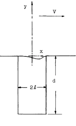
This solution can be obtained asymptotically, by an extension of the previous saddle point technique, from Eq. (3.1). It is first neces-sary to note, from Eqs. (3.5) or (3.10), that supersonic speeds imply an additional branch point in k0 as a function of 0 at the Mach angle. The proper branch is determined from the physical requirement that the field be zero outside the Mach cone. Inside the Mach cone, we can obtain out-going waves at infinity when the radical of Eq. (3.5) or of Eq. (3.10) has either positive or negative sign. This implies that there are two saddle points on the same Riemann surface. These saddle points tend to + and - oo as 0 approaches the Mach angle (sin 0 = I/ M). Thus, the branch point in k0 is at k + oo, and an appropriate cut is a large semicircle in the lower half of the k plane, as shown in Fig. 14. This cut excludes the values of k0 corresponding to 0 outside the Mach cone.

Thus, the supersonic evaluation of Eq. (3.1) gives two terms, corresponding to the two saddle points shown in Fig. 14. It is easily seen that the new saddle point has ft(k0) the opposite sign from the old saddle

00 M-A4osG // / [ACH ANGLE CUT \AT SADDLE PATH

ckp_ M+Acos

\

Ct) 2 _ M -1 I / / /

-,-.-

-Figure 14. SADDLE PATH FOR M>l WITH BRANCH CUT AT MACH ANGLE

ck

-0

This means that the supersonic evaluation of Eq. (3.1) is the sum of Eq. (3.13a) and a term identical with Eq. (3.13a) except for the sign of A 1 changed wherever it appears and a phase factor of +in/4 instead of - iir/4.

This analysis indicates that there is an extra term added to Eqs. (3.8), (3.9), (3.12), (3.13) for supersonic flow in the medium which the particular equation applies to. Equations (3.9) and (3.13) are written

in retarded coordinates, so the second term is identical in form with the term already given. But, since there are two retarded source points for the supersonic case, the second term refers to a coordinate system with the origin at the new second retarded source point. For Eqs. (3.8) and (3.12), the second term is obtained by taking the negative square root for A. (In addition, the phase must be shifted as is described above.) Both terms become equal (except for phase) at the Mach angle which is a branch point for the expressions in the instantaneous coordinate system. Beyond this point, the saddle point k0 obviously becomes complex, and

the causality condition requires that there be no sound field. This will be the case for the cut shown in Fig. 14.

V. Some Additional Terms for the Near Field

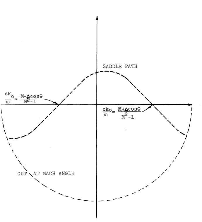
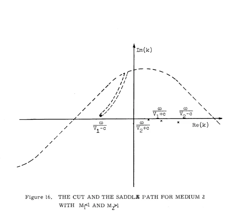
It was mentioned earlier that it is sometimes necessary to cross a branch point while moving the real k-axis to the saddle path in-dicated in Figs. 6 or 14. Examples of the proper distortion of the sad-dle path are given in Figs. 15 and 16. These examples are taken for the evaluation of 02, but the situation for

0,

is similar. It is evident from these figures that the effect of the distortion around the branch

CUT FOR Rey('y

M

-A cosG

22

2 _

..

M

₂

-1

- - - ol

)=0

/ I, /

//

'V

Im(k)

N

Re(k)

I

r-m

Figure 15. SADDLE PATH FOR 0

2 AND CUT FOR 0'

44

ck

-1i

/

//

U) V -c

Figure 16. THE CUT AND THE SADDLE PATH FOR MEDIUM 2 WITH Mi<l AND Mg>

45

Im(k)

/ / 1) v I+C _V 2 -c x w ~ v

2+c

/ x 7

Re(k)

point can be accounted for by the addition of the integral around the branch cut.

As a simple example, we set M= 0 and solve the integral

for q2. The necessity for the extra integral arises when ko is to the

left of the branch point for y = 0. Such a situation is shown in Fig. 15. It is convenient to integrate along both sides of the cut Reyl = 0. To do the integration for 02, it is convenient to make the change of variable

k2 = 2/C2 -u2 (which means ,= iu)

and approximate the integrand for small values of u. This assumes that the major contribution to the integral comes from the vicinity of the branch point u = 0. To this approximation,

k =

-(w/c)

+ (u 2c/2w) and

= (i/ c) q M2(2 + M + [icu2 1 - M - M 2+

With these substitutions, the integral becomes

S = 2 e(it+ (iy/c) - (icx/ c) N/ M(2 TM) -[(ic/2w) y+ [x( - M2-) 2c

Nf(23M1u AZ

7U[T/]]

[-iuh/[ iu 2 / 2)]

eiuh 2 2 udu

major contribution to the integral comes from u

<<

w/c, the integrand can be further simplified by neglecting u whereever it occurs in the de-nominator. Then, the integral may be evaluated in a straightforward manner to yield

= 8Nri 1h(l + M) eit+(y/c) [ x4M(2+YM)/c] + h2/2c([x(l-M 2 - M)/

N/ M(2+ M)] + y)

[wM(2+M)/C] ([x(1-M 2 -M)/'JM(2+M)] +y) 3/2 . (3.15)

It is evident that 02 becomes infinilefor

tan 0

= - 41M₂

(2

+

M

₂

)/(I

-

M

-

M

₂

)

*

This corresponds to the branch point k = w/c, being the same point as the saddle point k0. For larger angles, the saddle point will be to the

left of the branch point as depicted in Fig. 15, and 0 is added to the saddle point integration 02 to obtain the more complete solution. For smaller angles, the branch point is to the left of the saddle point, and

k

gives no contribution. This wave 0 is just in the zone of silence" as was predicted earlier. At the angle of the boundary of the Rzone of silence,'t given by (3.15a), q2 becomes a poor approximation just as the saddle point integration becomes a poor first-order approximation. This is to be expected, since the two integrations overlap as this criti-cal angle is approached.

k

₂ is a wave that travels most of the distance