HAL Id: hal-01954133
https://hal.univ-cotedazur.fr/hal-01954133
Submitted on 13 Dec 2018HAL is a multi-disciplinary open access archive for the deposit and dissemination of sci-entific research documents, whether they are pub-lished or not. The documents may come from teaching and research institutions in France or abroad, or from public or private research centers.
L’archive ouverte pluridisciplinaire HAL, est destinée au dépôt et à la diffusion de documents scientifiques de niveau recherche, publiés ou non, émanant des établissements d’enseignement et de recherche français ou étrangers, des laboratoires publics ou privés.
accuracy study
Richard Pasquetti, Francesca Rapetti
To cite this version:
Richard Pasquetti, Francesca Rapetti. Cubature points based triangular spectral elements: An accuracy study. Journal of Mathematical Study, Global Science Press, 2018, 51 (1), pp.15-25. �10.4208/jms.v51n1.18.02�. �hal-01954133�
Cubature points based triangular spectral elements:
An accuracy study
Richard Pasquetti∗, Francesca Rapetti
Universit´e Cˆote d’Azur, CNRS, Inria, Lab. J. A. Dieudonn´e, F-06108 Nice, France.
Abstract. We investigate the cubature points based triangular spectral element method and provide accuracy results for elliptic problems in non polygonal domains using various isoparametric mappings. The capabilities of the method are here again clearly confirmed.
Key Words: Spectral element method, simplicial meshes, cubature points, Fekete points, isopara-metric mappings.
AMS Subject Classifications: 65
Chinese Library Classifications: O175.27
1
Introduction
Extending the capabilities of the quadrangle based spectral element method to the trian-gle based one, say from the QSEM to the TSEM, has received a considerable attention in the last twenty years. The relevant choice of interpolation points for the triangle has thus motivated a lot of works, see e.g. the Review paper [15] and references herein. Sev-eral sets of points have indeed been proposed, some of them showing the advantage of simplicity in their generation, thus allowing an easy extension to the tetrahedron, e.g.the so-called warp & blend points [21], whereas some other ones are more satisfactory from the theoretical point of view, e.g.the celebrated Fekete points of the triangle, but much more difficult to compute [20].
With respect to the QSEM, based on the use of the tensorial product of Gauss-Lobatto-Legendre (GLL) nodes, such interpolation points are however not quadrature points, so that the so called spectral accuracy gets lost if not using for the quadratures a separate set of points, as e.g.done for the Fekete-Gauss approach [14]. Using two separate sets of points shows however some drawbacks, because the mass matrix is then no longer diagonal. Thus, when solving an evolution problem with an explicit time scheme, one has at each time step to solve a mass matrix algebraic system. Also, a diagonal mass
∗Corresponding author. Email address: [email protected] (R. Pasquetti)
matrix can be useful to set up high order differentiation operators [12]. This is why it is of interest to design a TSEM that makes use of a single set of points showing both nice quadrature and interpolation properties. This was the goal of the cubature points based TSEM, as developed in the last few years [2, 5, 9, 13].
Another difficulty with SEMs, and more generally with high order FEMs, is to main-tain the accuracy when the computational domain is no longer polygonal. Several strate-gies have been proposed to handle curved elements, from transfinite mappings [6] to PDEs based transformations, e.g.the harmonic extension.
The present work follows two anterior studies:
• In [16], using the Fekete-Gauss TSEM we compared different strategies for curved triangular spectral elements, i.e. when isoparametric mappings are required to cor-rectly approximate with curved spectral elements the presence of a curved bound-ary.
• In [17], for computational domains of polygonal shape we compared the cubature TSEM, as proposed in [9], and the Fekete-Gauss one. In terms of accuracy for ellip-tic problems, it turned out that these two TSEMs compare well. With non Dirichlet or non homogeneous Neumann conditions, i.e. as soon as boundary integrals are involved, some care is however needed if using the cubature TSEM.
Here the goal is to extend the results obtained in [16] to the case where the cubature TSEM is used. As in [16, 17] we only focus on elliptic problems, but keep in mind for future works the inherent difficulties associated to constrained operators, see e.g. [1].
2
Cubature points based
TSEM
For the sake of completeness, let us recall that [17]:
• If two different sets of points are used for interpolation and quadrature, then the space PN(Tˆ)of polynomials of maximal (total) degree N, defined on the reference triangle ˆT= {(r,s):r∈ (−1,1),s∈ (−1,−r)}, is usually used as approximation space. The cardinality of this space equals n=(N+1)(N+2)/2, that can be associated to n interpolation points if using Lagrange polynomials as basis functions. If 3 of these nodes coincide with the vertices of the element, then 3N of these n points should belong to the edges of ˆT and the remaining(N−1)(N−2)/2 are the inner nodes. Usually, the edge nodes proposed in the literature coincide with the GLL points. Since one does not know an explicit formulation of the Lagrange basis functions, say ϕi(r,s), 1≤i≤n, to compute their values or those of their derivatives at given point one generally makes use the orthogonal Kornwinder-Dubiner (KD) basis [4], for which explicit formula exist. Gauss points for the triangle and the correspond-ing quadrature formula may be found in the literature, up to degree M≈20 if a symmetric distribution of the points is desired. In practice, one may choose M=2N,
so that both the stiffness and mass matrix are exactly computed, since their entries are polynomials of degree 2N and 2N−2, respectively. For details on the imple-mentation of the Fekete-Gauss approach, see e.g. [14].
• If using a single set of points, as before 3N of the interpolations points must belong to the triangle boundary with 3 of them at the vertices. As demonstrated in [7, 22], such a strong constraint forbids the possibility of finding a set of cubature points providing a sufficiently accurate cubature formula, if looking for basis functions that span the space PN. To overcome this difficulty, as first developed in [2], the idea is then to enrich the space PNby polynomial bubble functions of degree N′>N. This indeed allows to include new cubature points inside the triangle while keep-ing the element boundary nodes number equal to 3N. In the reference triangle ˆT, this may be achieved by introducing the polynomial space PN∪b×PN′−3, where b is the (unique) bubble function of P3(Tˆ), namely b(r,s) = (r+1)(s+1)(r+s). The cardinality of this space then equals n′=3N+(N′−1)(N′−2)/2. Now, to compute the Lagrange polynomials at a given points one should use an extended KD ba-sis, composed of the usual KD basis of PN completed by those KD polynomials of
P
N′−3which once multiplied by the bubble function b are of degree strictly greater than N. Of course, N′ should be chosen as small as possible to avoid a useless in-crease of the inner nodes number: In [2] and posterior works, N′is chosen such that it exists a cubature rule exact for polynomials of degree N+N′−2. The determina-tion of N′, together with the cubature points and weights gives rise to a difficult optimization problem, see [9] for details. It turns out that N′−N increases mono-tonically with N: N′=N+1, for 1<N<5, N′=N+2 for N=5 and N′=N+3 for
5<N<10. It should be noticed that with the cubature TSEM, neither the mass
ma-trix nor the stiffness mama-trix are exactly computed, since their entries are of degree 2N′ and 2N′−2, respectively.
Our in house Fekete-Gauss and cubature codes make use of the condensation technique, i.e. one first computes the unknowns associated to the edges of the elements and then reconstructs the numerical solution inside locally. Thus, the algebraic systems that result from the two TSEM approximations are exactly of same size, and so the computational times compare well. They are simply solved by using a standard conjugate gradient method, with Jacobi preconditioner in a matrix free implementation [8].
A difficulty however arises when the boundary conditions are not of Dirichlet or ho-mogeneous Neumann type, i.e. when the weak formulation involves boundary integrals. In case of the Fekete-Gauss TSEM, such boundary integrals can be easily computed since the edge Fekete nodes coincide with the GLL points. On the contrary, the edge cubature points are not of Gauss type. In [17],
• it is pointed out that for the Robin condition ∂nu+αu=g, g being a given function and α a coefficient possibly zero, using a quadrature rule based on the boundary cubature points is not satisfactory,
• it is suggested to approximate these integrals by using on each element edge of the boundary a Gauss quadrature rule, e.g.the one based on the GLL points.
Since the restrictions of the Lagrange polynomials ϕi at the element edges of the bound-ary are polynomials of degree N, one can span this polynomial space with the Legendre polynomials, say Li(r)with r∈ [−1,1], for the reference edge, and 0≤i≤N. Then, one can set up the Vandermonde matrices of size(N+1)×(N+1)based on the cubature and GLL points, say VCuband VGLL. One has e.g.(VCub)ij=Lj(ri), with ri∈ [−1,1]for the edge cubature points. Then, the matrix VGLLVCub−1 allows to compute at the GLL points quan-tities known at the cubature points. Especially, each column of this matrix provides the values of the edge Lagrange polynomials at the GLL points.
Another difficulty arises with curved spectral elements. Indeed, for straight triangu-lar elements, the edge Jacobian determinant is constant on each edge and proportional to its length. On the contrary, when considering curved triangular elements, some care is needed for a relevant computation of the edge Jacobian determinants at the GLL points from those at the cubature points. Thus, once the entries of the Jacobian matrix have been computed at the edge cubature points, one can
• compute the edge Jacobian determinant and then use the polynomial interpolation to get the Jacobian at the GLL points,
• use the polynomial interpolation to get the Jacobian matrix entries at the GLL points and then compute the Jacobian determinant.
Because the edge Jacobian determinant is generally a polynomial of degree greater than N, the results of these two approaches slightly differ. There is indeed no interpolation error for the Jacobian matrix entries but there is such an error for the Jacobian matrix determinant. This is why in our cubature points based solver, it is the second approach which is implemented, even if a little more expensive than the first one.
3
Isoparametric mappings
For the cubature TSEM, hereafter we make use of the isoparametric mappings that we discussed in [16]:
• The bending procedure that we introduced in [8];
• The transfinite interpolation discussed for the triangles in [18]; • The harmonic extension;
Moreover, local mappings are used, i.e. we simply distort the elements at the boundary. As in [16], we assume to have at hand a parametric description of the boundary of Ω, i.e. , Γ is defined by a vector function, say xΓ(t) = (xΓ(t),yΓ(t)), where t∈ [tmin,tmax]. Let
A1A2A3be a triangular element at the boundary, with A1the inner node and A2and A3
on the boundary. Then, for all the four approaches it is assumed that the boundary nodes, i.e. the interpolation points of Γ, are at the intersection of the lines joining the inner vertex A1and the interpolation points of the straight line A2A3, i.e. the edge of the element, say
˜
T, provided by the piecewise linear P1mapping. This requires one to solve, in general
using a simple numerical procedure, N−1 (number of nodes of an edge without the end points) generally non-linear equations. Then, it remains to define n′pinner interpolation points, with n′p=n′−3N= (N′−1)(N′−2)/2, for the cubature TSEM.
For the paper to be self contained, let us briefly describe the previously mentioned isoparametric mappings [16]:
• The bending procedure: Assume that ˜F is the interpolation point obtained with the affine P1mapping. Let ˜G and G be the points at the intersections of A1F with˜
the line A2A3 and the boundary Γ, respectively. Then, the bending procedure [8]
consists of stating that F is homothetic to ˜F by the homothety of center A1 and of
ratio A1G/A1G, so that:˜
A1F=A1G
A1G˜
A1˜F and d≡˜FF= (A1G
A1G˜
−1)A1˜F
where d stands for displacement. One notices that for this bending procedure, only the point G of Γ influences the location of the interpolation point F. In order to define the inner interpolation points, one has numerically to solve n′pequations. • The transfinite interpolation: For the triangle, the method makes use of the
barycen-tric coordinates, say (λ1,λ2,λ3). Recall that λi=0 stands for the edge opposite to the vertex i, λi=Constant to a line parallel to this edge and that vertex i belongs to λi=1. General transfinite interpolation formula are given in [18] (different approaches are however possible, see e.g. [3]). For the triangle, if the displacement d vanishes at the two edges A1A2 and A1A3, again assuming that
⌢
A2A3 is the curved edge, one
has:
d(λ1,λ2,λ3) =λ2d(0,1−λ3,λ3)+λ3d(0,λ2,1−λ2).
This means that two points of the boundary Γ influence the location of an inner interpolation point F. They are those at the intersections of Γ with the lines parallel to A1A2and A1A3and passing by the point ˜F. One notices that the method requires
solving 2n′pequations.
• Harmonic extension: The goal is here to define the inner interpolation points by solving, for each curved element T, the weak form of the Laplace Dirichlet problem:
∆d=0 in ˜T, d| ∂ ˜T=g
with g given on A2A3and g=0 on the two other sides. To resolve this vector Laplace
problem, that in fact yields two uncoupled scalar problems, one has to set up the differentiation matrices, say D˜x and D˜y that allows one to compute derivatives in
˜
T. To this end, one makes use of the differentiation matrices Drand Dsand applies the chain rule. Since the mapping from ˆT to ˜T is affine, the Jacobian matrix and Jacobian determinant are constant. For the same reason, one may solve directly for the interpolation point coordinates. Finally, one should invert a matrix of size n′p×n′p, in order to compute the coordinates of the inner interpolation points. The approach is thus rather simple and in practice not costly. In [11], where global mappings are considered, it is however outlined that the harmonic extension may fail to define a mapping.
• Linear elasticity: Here the curved domain is viewed as the deformation of triangles, that is governed by the equation of linear elasticity. Introducing the Lame coeffi-cients λ and µ, the displacement field is governed by the Navier-Cauchy equation:
µ∆d+(λ+µ)∇(∇·d) =0 in ˜T, d|∂ ˜T=g.
There is now a coupling between the components of the displacement field. Using the ingredients previously described for the harmonic extension, the weak form of this elasticity problem yields a matrix system of size 2n′p. The solution of this system provides the displacements of the inner interpolation points. Again, one can also compute directly their coordinates. Because the forcing term is zero, the mapping is here parametrized by the ratio µ/(λ+µ) =1−2η, where η∈ (−1,0.5)is the so called Poisson ratio.
4
Accuracy study
First, one of the test-cases introduced in [16] has been revisited. Using the cubature TSEM we solve the Poisson equation, −∆u= f , with exact solution uex=cos(10x)cos(10y), so that f =200uex, and Dirichlet boundary conditions, in the computational domain and mesh (the so-called medium mesh of [16]) presented in Fig. 1 (left). For the elasticity isoparametric mapping, the Poisson ratio is taken equal to 0.2.
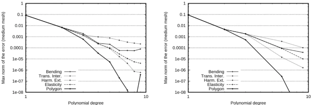
For the different isoparametric mappings, the max norm of the error, obtained from the errors at the cubature points, is shown in Fig. 2 (left). The curve labeled “polygon” is the one obtained for the domain defined by the P1mesh, i.e. no isoparametric mapping
is involved in this case. Such results compare well with those obtained with the Fekete-Gauss TSEM, recalled in Fig. 2 (right). Again, one observes that the best results are obtained with the harmonic extension or with the linear elasticity approach, i.e. with the isoparametric mappings based on PDEs rather than transfinite interpolations. As in [17], one observes that a loss of accuracy occurs for N=9. It is due to a slight lack of accuracy of the cubature rule [10].
Figure 1: Computational domains and corresponding P1meshes. 1e-08 1e-07 1e-06 1e-05 0.0001 0.001 0.01 0.1 1 1 10
Max norm of the error (medium mesh)
Polynomial degree Bending Trans. Inter. Harm. Ext. Elasticity Polygon 1e-08 1e-07 1e-06 1e-05 0.0001 0.001 0.01 0.1 1 1 10
Max norm of the error (medium mesh)
Polynomial degree Bending Trans. Inter. Harm. Ext. Elasticity Polygon
Figure 2: Max norm of the error vs the polynomial degree N for the Poisson-Dirichlet problem using the cubature
TSEM (at left) and the Fekete-Gauss TSEM (at right).
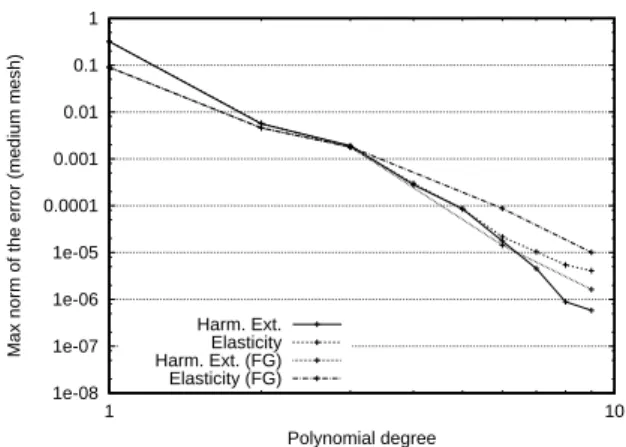
Rather than the Dirichlet condition, we now use the Robin condition ∂nu+u=g, with g derived from the exact solution uex=cos(10x)cos(10y). Results obtained with the Fekete-Gauss solver and with cubature points based solver are compared in Fig. 3, using the PDEs based isoparametric mappings (harmonic extension and linear elasticity). Clearly, the results obtained with the Fekete-Gauss and the cubature TSEM compare well. Thus, even if curved elements are involved, if the boundary data are correctly handled [16] then the cubature approach proposed in [9] is quite satisfactory (at least for N≤8).
To extend the present study we consider the computational domain and P1-mesh
1e-08 1e-07 1e-06 1e-05 0.0001 0.001 0.01 0.1 1 1 10
Max norm of the error (medium mesh)
Polynomial degree Harm. Ext.
Elasticity Harm. Ext. (FG) Elasticity (FG)
Figure 3: Max norm of the error vs the polynomial degree N for the Poisson-Robin problem using the cubature
TSEM and the Fekete-Gauss TSEM.
angle θ:
x = cosθ(1+0.3 cos(7θ))
y = sinθ(1+0.2 cos(7θ)).
The P1-mesh is generated from 50 boundary nodes, defined by θ∝2π/50, and the number
of elements equals 174.
Isoparametric mappings based on the harmonic extension and linear elasticity ap-proaches are used. Till now, the linear elasticity isoparametric mapping was character-ized by a Poisson ratio η=0.2. Then, it is of interest to carry out a sensitivity study to this parameter. For isotropic materials one has η∈ (−1,0.5), most materials are such that η∈ (0,0.5), and for typical engineering materials η∈ (0.2,0.5). Hereafter we make computations with the following Poisson ratio η= {0.1,0.2,0.4}.
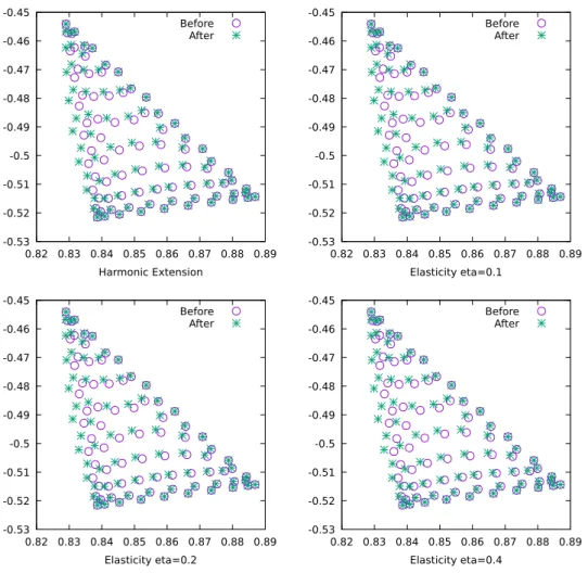
For one particular element of the mesh and a polynomial approximation degree N=6, Fig. 4 shows the distribution of the cubature nodes obtained from the P1-mapping and
from the isoparametric P6-mapping, when using the harmonic extension or the linear
elasticity mappings associated to the different Poisson ratio.
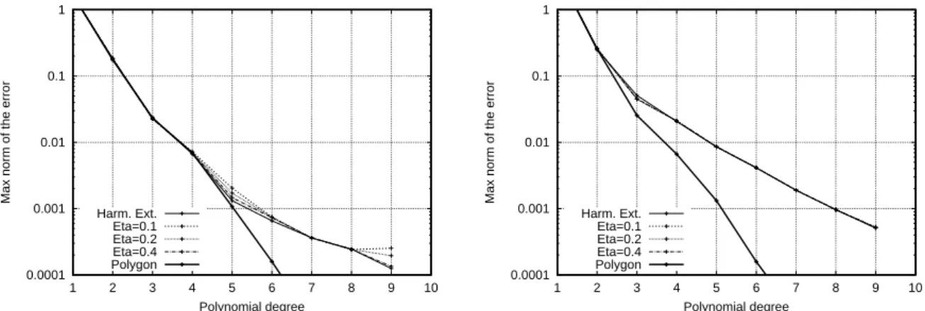
We make use of the cubature TSEM and the exact solution uex=cos(10x)cos(10y)to set up the source and boundary terms, f and g, of the following elliptic PDE−∆u+u=f . Accuracy tests are made using Dirichlet conditions, i.e. u=g at the boundary nodes, and also the Robin condition ∂nu+u=g. The results obtained for these Dirichlet and Robin problems are shown in Fig. 5, at left and at right, respectively.
One observes that:
• For the linear elasticity isoparametric mapping, the sensitivity to the Poisson ratio η is low. With the Robin condition, all curves coincide. With the Dirichlet condition, one can discern a slight improvement for the largest value η=0.4, the convergence
-0.53 -0.52 -0.51 -0.5 -0.49 -0.48 -0.47 -0.46 -0.45 0.82 0.83 0.84 0.85 0.86 0.87 0.88 0.89 Harmonic Extension Before After -0.53 -0.52 -0.51 -0.5 -0.49 -0.48 -0.47 -0.46 -0.45 0.82 0.83 0.84 0.85 0.86 0.87 0.88 0.89 Elasticity eta=0.1 Before After -0.53 -0.52 -0.51 -0.5 -0.49 -0.48 -0.47 -0.46 -0.45 0.82 0.83 0.84 0.85 0.86 0.87 0.88 0.89 Elasticity eta=0.2 Before After -0.53 -0.52 -0.51 -0.5 -0.49 -0.48 -0.47 -0.46 -0.45 0.82 0.83 0.84 0.85 0.86 0.87 0.88 0.89 Elasticity eta=0.4 Before After
Figure 4: Distribution of the cubature nodes before and after the isoparametric mapping: Harmonic extension (top left), elasticity with η=0.1 (top right), η=0.2 (bottom left) and η=0.4 (bottom right)
curve being then the closest to the harmonic extension one. Note that this is sur-prising, since if η→0.5 then µ→0.
• The decrease of the error for the Robin problem is exponential, whereas this is less obvious in the Dirichlet case. In fact, the convergence curves show two parts, be-low and beyond a critical value of the polynomial degree. Roughly speaking, for the smallest values of N the convergence rate is governed by the approximation of the solution in the bulk of the domain, whereas for the largest ones it is enforced by its approximation at the boundary. This is why, see Fig. 5, for small N the conver-gence curves coincide with those obtained when using as computational domain the polygon obtained from the 50 boundary nodes, but differ for N larger than threshold values, say, for the present P1 discretization of the star-shaped domain,
0.0001 0.001 0.01 0.1 1 1 2 3 4 5 6 7 8 9 10
Max norm of the error
Polynomial degree Harm. Ext. Eta=0.1 Eta=0.2 Eta=0.4 Polygon 0.0001 0.001 0.01 0.1 1 1 2 3 4 5 6 7 8 9 10
Max norm of the error
Polynomial degree Harm. Ext. Eta=0.1 Eta=0.2 Eta=0.4 Polygon
Figure 5: Max norm of the error vs the polynomial degree N, using the cubature TSEM for an elliptic problem in the star domain, with Dirichlet (at left) and Robin (at right) conditions.
N=5 and N=3 with Dirichlet and Robin conditions, respectively.
Acknowledgments
The P1FEM meshes have been generated with the free software “Triangle”. We are
grate-ful to Dr Youshan Liu, Chinese Academy of Sciences, Beijing, for transmitting us the cubature points and weights used in [9].
References
[1] E. Ahusborde, R. Gruber, M. Azaiez and M.L. Sawley, Physics-conforming constraints-oriented numerical method, Phys. Rev. E, 75 (2007), 056704.
[2] G. Cohen, P. Joly, J.E. Roberts and N. Tordjman, Higher order triangular finite elements with mass lumping for the wave equation, SIAM J. Numer. Anal., 38 (2001), 2047-2078.
[3] L. Demkowicz, J. Kurtz, D. Pardo, M. Paszynski, W. Rachowicz and A. Zdunek, Computing with hp-adaptative finite elements, vol. 1, Chapman & Hall / CRC, 2007.
[4] M. Dubiner, Spectral methods on triangles and other domains, J. Sci. Comput., 6 (1991), 345-390.
[5] F.X. Giraldo and M.A. Taylor, A diagonal mass matrix triangular spectral element method based on cubature points, J. of Engineering Mathematics, 56 (2006), 307-322.
[6] W.J. Gordon and C.A. Hall, Construction of curvilinear co-ordinate systems and applications to mesh generation, Int. J. Num. Methods in Eng., 7 (1973), 461-477.
[7] B.T. Helenbrook, On the existence of explicit hp-finite element methods using Gauss-Lobatto integration on the triangle, SIAM J. Numer. Anal., 47 (2009), 1304-1318.
[8] L. Lazar, R. Pasquetti and F. Rapetti, Fekete-Gauss spectral elements for incompressible Navier-Stokes flows: The two-dimensional case, Comm. in Comput. Phys., 13 (2013), 1309-1329.
[9] Y. Liu, J. Teng, T. Xu and J. Badal, Higher-order triangular spectral element method with optimized cubature points for seismic wavefield modeling, J. of Comput. Phys., 336 (2017), 458-480.
[10] Y. Liu, private communication (2017).
[11] A.E. Løvgren, Y. Maday and E.M. Ronquist, Global C1maps on general domains, Mathe-matical Models and Methods in Applied Sciences, 19 (5) (2009), 803-832.
[12] S. Minjeaud and R. Pasquetti, High order C0-continuous Galerkin schemes for high order PDEs, conservation of quadratic invariants and application to the Korteweg-De Vries model, J. of Sci. Comput., (2017), https://doi.org/10.1007/s10915-017-0455-2 .
[13] W.A. Mulder, New triangular mass-lumped finite elements of degree six for wave propaga-tion, Progress in Electromagnetic Research, 141 (2013), 671-692.
[14] R. Pasquetti and F. Rapetti, Spectral element methods on unstructured meshes: comparisons and recent advances, J. Sci. Comp., 27 (1-3) (2006), 377-387.
[15] R. Pasquetti and F. Rapetti, Spectral element methods on simplicial meshes, Lecture Notes in computational Science and Engineering : Spectral and High Order Methods for Partial Differential Equations - ICOSAHOM 2012, 95, Springer (2014), 37-55.
[16] R. Pasquetti, Comparison of some isoparametric mappings for curved triangular spectral elements, J. of Comput. Phys., 316 (2016), 573-577.
[17] R. Pasquetti and F. Rapetti, Cubature versus Fekete-Gauss nodes for spectral element meth-ods on simplicial meshes, J. of Comput. Phys., 347 (2017), 463-466.
[18] A. Perronnet, Triangle, tetrahedron, pentahedron transfinite interpolations. Application to the generation of C0 or G1-continuous algebraic meshes, Proc. Int. Conf. Numerical Grid Generation in Computational Field Simulations, Greenwich, England (1998), 467-476. [19] P.O. Persson and J. Peraire, Curved Mesh Generation and Mesh Refinement using
La-grangian Solid Mechanics, Proc. of the 47th AIAA Aerospace Sciences Meeting and Exhibit, January 2009. AIAA-2009-949.
[20] M.A. Taylor, B. Wingate and R.E. Vincent, An algorithm for computing Fekete points in the triangle, SIAM J. Numer. Anal., 38 (2000), 1707-1720.
[21] T. Warburton, An explicit construction for interpolation nodes on the simplex, J. Eng. Math., 56 (3) (2006), 247-262.
[22] Y. Xu, On Gauss-Lobatto integration on the triangle, SIAM J. Numer. Anal., 49 (2011), 541-548.