HAL Id: hal-01120734
https://hal.inria.fr/hal-01120734
Submitted on 26 Feb 2015
HAL is a multi-disciplinary open access
archive for the deposit and dissemination of
sci-entific research documents, whether they are
pub-lished or not. The documents may come from
teaching and research institutions in France or
abroad, or from public or private research centers.
L’archive ouverte pluridisciplinaire HAL, est
destinée au dépôt et à la diffusion de documents
scientifiques de niveau recherche, publiés ou non,
émanant des établissements d’enseignement et de
recherche français ou étrangers, des laboratoires
publics ou privés.
Hybrid Automatic Visual Servoing Scheme using
Defocus Information for 6-DoF Micropositioning
Le Cui, Eric Marchand, Sinan Haliyo, Stéphane Régnier
To cite this version:
Le Cui, Eric Marchand, Sinan Haliyo, Stéphane Régnier. Hybrid Automatic Visual Servoing Scheme
using Defocus Information for 6-DoF Micropositioning. IEEE Int. Conf. on Robotics and Automation,
ICRA’15, May 2015, Seattle, United States. �hal-01120734�
Hybrid Automatic Visual Servoing Scheme using Defocus Information
for 6-DoF Micropositioning
Le Cui
1, Eric Marchand
1, Sinan Haliyo
2and St´ephane R´egnier
2 Abstract— Direct photometric visual servoing uses only thepure image information as a visual feature, instead of using classic geometric features such as points or lines. It was demonstrated efficiently in 6 degrees of freedom (DoF) posi-tioning. However, in micro-scale, using only image intensity as a visual feature performs unsatisfactorily in cases where the photometric variation is low, such as motions along vision sensor’s focal axis under a high magnification. In order to improve the performance and accuracy in those cases, an approach using hybrid visual features is proposed in this paper. Image gradient is employed as a visual feature on z axis while image intensity is used on the other 5 DoFs to control the motion. A 6-DoF micro-positioning task is accomplished by this hybrid visual servoing scheme. The experimental results obtained on a parallel positioning micro-stage under a digital microscope show the robustness and efficiency of the proposed method.
I. INTRODUCTION
Automatic and reliable positioning, handling and assembly of the micro-structures have shown their potential in fabrica-tion of micro-structures and microelectromechanical systems (MEMS) over the past few decades. In the micro-scale, the prevailing spatial sensing technique is vision, through optical or electron microscopy. Visual servoing is hence an unavoidable tool to automate manipulation tasks [1], [2]. The accuracy in position and orientation of a sample in the camera reference frame is one important issue [3], [4]. Many approaches in this domain rely the observation of object features [5], [6]. The pose (i.e., position and orientation) of samples is computed by estimating the position and orientation of these features. Furthermore, available imaging techniques at the micro-scale by an optical or electronic microscope exhibit several limitations such as high signal-to-noise ratio, low refresh rate, contrast, etc., leading to the bottleneck of pose detection.
Recently, a novel visual servoing technique has been proposed to overcome these different issues. This approach uses the photometric information [7], [8] as a visual feature in the image based control law. In this case, only the image intensity is needed while visual tracking, including feature extraction and motion prediction is no longer necessary. This approach is demonstrated in micro-positioning on 3-DoF (translation along x and y axes, and rotation around z
1Le Cui and Eric Marchand are with Universit´e de Rennes 1,
La-gadic group, IRISA, Rennes, [email protected], [email protected]
2Sinan Haliyo and St´ephane R´egnier are with
Sor-bonne Universit´es, UPMC Univ Paris 06, UMR 7222,
ISIR, Paris, France [email protected],
axis) [9], and on 6-DoF with some limitations on translation along z axis [10].
Particularly in micro-nano scale, the motion along z axis is difficult to observe due to microscope projection model [11]. As a microscope provides a long focal length, a motion along z axis causes only a tiny variation on the observed image. Using only image intensity information as a visual feature, the accuracy of the translation on z axis is inferior to other DoFs. Accurate depth information is an important issue for correct positioning. Many approaches in depth detection have been proposed in computer vision. One idea is to employ stereo vision and reconstruct the tree-dimensional (3D) image from several two-dimensional (2D) images [12], in which the reliable extraction of features is necessary. Both extraction and feature matching could be computationally expensive. Considering focus information, depth from focus (DFF) [13] has been proposed. The basic of this method is to obtain different focus levels by adjusting the camera parameters (i.e., the distance between the lens and image plane, the focal length and the aperture radius). It involves obtaining many observations for the various camera param-eters and estimating the focus using a criterion function. Since many camera parameters and observations should be considered, it is not practical in positioning. Alternatively, the depth from defocus (DFD) based approaches have been also widely discussed [14], [15]. The main idea of these methods is objects at a particular distance from the lens will be focused in an optical system, whereas objects at other distances will be blurred. By measuring the amount of defocus of the object on the observed image, the depth of the object with respect to the lens can be recovered from the geometric optics. In these methods, the defocus parameters can by estimated from the image by an inverse filter in the Fourier domain [14], by modeling the depth and the image as separate Markov random fields [16], or by some spatial domain-based techniques [17], etc. Inspired from the DFD, considering that the image sharpness and focus vary significantly when using an optical path which provides a small depth of field, the image gradient information can be hence used for controlling z motion in a visual servoing scheme.
This study addresses a closed-loop control scheme for visual servoing using image intensity and image gradient for a micro-positioning task in 6-DoF. The proposed method is demonstrated experimentally on a 6-DoF parallel-kinematics positioning stage and a digital microscope. The manuscript is organized as follows: Section II briefly recalls the classic visual servoing and introduces the general approach. Section
III describes selected visual features, image intensity and gradient. The hybrid control laws constructed with these features are presented in Section III C. Experimental results obtained on a 6-DoF parallel micro-assembly workcell are shown in Section IV.
II. CLASSICAL VISUAL SERVOING
Two distinct robot-camera relation cases exist in classical visual servoing [18]: eye-in-hand case, in which the camera is installed in the end-effector, and alternatively, the eye-to-hand case, where the camera is fixed and look toward the end-effector. In micro/nano-robotics, the eye-to-hand case is generally considered since the sensor (microscope) is usually motionless.
In classical visual servoing, the objective is to minimize
the error e between the current visual feature s(q) and the
desired ones⇤:
e(q) = s(q) s⇤ (1)
The relation between the time derivative ˙s and the robot
joint velocity ˙q is given by:
˙
s = Jsq˙ (2)
whereJs represents the visual feature Jacobian.
With an exponential decrease of the error ˙e = e, with
(1) and (2), the control law can be expressed as: ˙
q = J+
se (3)
where is the proportional coefficient andJ+
s is the
pseudo-inverse ofJs.
Considering the eye-to-hand visual servoing context, the
Jacobian Js can be expressed as:
Js= LscVFFJn(q) (4)
whereLs represents the interaction matrix, which links the
relative camera instantaneous velocityv and the feature
mo-tion ˙s,cV
F is the motion transform matrix which transforms
velocity expressed in camera reference frame onto the robot
frame, FJ
n(q) is the robot Jacobian in the robot reference
frame.
To improve the robustness of algorithm, a Levenberg-Marquardt-like method is considered:
˙
q = (H + µ · diag(H)) 1J>se(q) (5)
where µ is a coefficient whose typical value ranges from 0.001 to 0.0001. diag(H) represents a diagonal matrix of
the matrixH = J>
sJs.
III. PURE IMAGE INFORMATION BASED VISUAL
FEATURES
In visual servoing, one or more feature information, such as geometric measurements (e.g. position and orientation of interesting points) or direct image information including image gradient [19],[20] and image entropy [21] can be extracted as visual features. In [9],[10], the photometric in-formation is shown to be efficient for 6-DoF visual servoing. However, the accuracy of translation along z axis is much
inferior to others due to the lack of observation on z axis in micro/nano imaging: At high magnifications, existing models assume an orthogonal projection hence the output image varies slowly over the object/camera distance. In this paper a hybrid approach with features extracted from the pure image information is proposed for 6-DoF visual servoing. The general idea is to use image gradient information for controlling the motion on z axis and to use image intensity information to control the other degrees of freedom. A. Image intensity as a visual feature
First considering the intensity of all the pixels I from the
pure image as the main visual features, the cost function is
defined as:
eI(q) = I(q) I⇤ (6)
For a pixelx = (x, y) on image plane, the time deviation of
x can be expressed by ˙
x = Lxv. (7)
wherev = (v, w) contains the relative camera instantaneous
linear velocity v and angular velocity w,Lxis the interaction
matrix:
Lx=
1
Z 0 xy (1 + x2) y
0 Z1 1 + y2 xy x . (8)
Let I(x, t) be the intensity of the pixel x at time t, then rI =
@I
@x 0
0 @I@y , (9)
the total deviation of the intensity I(x, t) can be written as ˙
I(x, t) = rI ˙x + ˙I, (10)
where ˙I = @I
@t represents the time variation of I. According
to [22] based on the temporal luminance constancy hypoth-esis, ˙I(x, t) = 0. In this case,
˙
I = rILxv = LIv. (11)
Considering the entire image, I = (I00, I01,· · · , IM N),
where M, N represent the image size: ˙I = 0 B @ LI00 ... LIM N 1 C A v = LIv (12)
where ˙I is the variation of the whole image intensity. LIis a
M N⇥ 5 matrix that theoretically allows a control law able
to compute the 5 DoFs.
B. Image gradient as a visual feature
As mentioned before, one difficulty in micro/nano vision at a high magnification is the lack of observation on z axis. Actually, for a sensor with small depth of field, it is evident that the image sharpness changes when z position changes. That leads the motion on z can be controlled according to the image sharpness. Hence, the image gradient is chosen as a visual feature to control the motion along z axis. An approach employing image gradient information in visual
servoing is proposed in this part. The general idea is to consider that the image gradient varies when object position on z axis changes, where the focal length of the sensor is always a constant. Practically, for a sensor with a small depth of field, the focal length of sensor can be adjusted in order to acquire a sharp image at the desired pose. In this case, the aim is to minimize the error of image gradient between the image at current pose and the image at desired pose to move the object to the target pose.
The linear image formation model, which is commonly used in the case of optical sensors [13] is employed here. Let Z be the current position on z axis, the defocus image I(x, y, Z) at the position Z can be expressed as the
convo-lution of a sharp imageI⇤(x, y, Z⇤) at the desired pose Z⇤
and a defocus kernel f(x, y):
I(x, y, Z) = I⇤(x, y, Z⇤)⇤ f(x, y) (13)
In previous studies, such as [23], the Gaussian kernel is widely used as an approximation of defocus model by many authors. Its probability density function (PDF) can be expressed by
f (x, y) = 1
2⇡ 2e
x2 +y2
2 2 . (14)
For a small displacement dZ on z axis, consider a propor-tional relation between d and dZ:
d = mdZ. (15)
where m is a constant coefficient.
For an imageI(x, y, Z) at Z on z axis, the square of the
norm of the image gradient at a point (x, y) on the image plane is
g(x, y, Z) =krI(x, y, Z)k2
=rI2
x(x, y, Z) +rIy2(x, y, Z)
(16) Considering the square of the norm of the image gradient for the whole image as the visual feature:
G(Z) = M X x=0 N X y=0 g(x, y, Z) = M X x=0 N X y=0 (rIx2(x, y, Z) +rIy2(x, y, Z)) (17)
One goal is then to minimize the error of the current image
gradient G(Z) and the desired image gradient G⇤(Z⇤). In
this case, the cost function is defined as:
eG(Z) = G(Z) G⇤(Z⇤) (18)
The relation between the relative camera instantaneous linear
velocity vz along z axis and the time variation of image
gradient G is
˙
G = LGvz (19)
where LG is the Jacobian (hence a scalar) which can be
expressed by: LG= @G @ @ @Z (20) From (15), it leads to LG= m @G @ . (21) where @G @ can be expressed by @G @ = M X x=0 N X y=0 2(rIx(x, y) @rIx(x, y) @ +rIy(x, y) @rIy(x, y) @ ) (22)
In (13), the convolution can also be written as:
I(x, y) =X
u
X
v
I⇤(x u, y v)f (u, v). (23)
From (14), compute the derivative @f (u, v) @ = 1 2⇡(u 2+ v2 2 2) 5e u2 +v22 2 . (24) According to (23) and (24): @rIx(x, y) @ = X u X v r(Ix⇤(x u, y v) · 2⇡1 (u2+ v2 2 2) 5e u2 +v22 2 ) (25) and @rIy(x, y) @ = X u X v r(I⇤ y(x u, y v) · 2⇡1 (u2+ v2 2 2) 5e u2 +v22 2 ) (26)
Considering (25) and (26) in (22), LG can be finally
com-puted.
C. Control law for hybrid visual servoing
For the hybrid visual servoing, both image intensity and image gradient are considered as visual features s =
(I(q), G(Z))>. Using image intensity as a visual feature,
the velocities (the linear and angular velocities on x, y axes, and the angular velocity around z axis) of the end-effector can be computed from (4), where the Jacobian is
JI = LIcVFFJn(q). (27)
Similarly, using image gradient as a visual feature, the linear velocity along z axis is:
˙
Z = zLG1eG(Z) (28)
where z is an exponential coefficient. During the visual
servoing process, the control laws for motion along z axis and the other 5 DoFs are computed respectively and simul-taneously.
Fig. 1. The micropositioning workcell
Y
X Z
O
Fig. 2. Parallel positioning stage
IV. EXPERIMENTALRESULTS
A. Experimental setup
Experiments are accomplished on a micropositioning workcell installed on an anti-vibration table shown in Fig. 1.
It contains a 6-DoF positioning-kinematics micro-stage 1 as
well as its modular control system and a digital microscope2
with an aperture-adjustable lens towards the top-plate of positioning stage. Experiments are realized on an optical magnification of 60⇥.
TABLE I
POSITIONING STAGE SPECIFICATIONS
Travel range Closed-loop resolution
X +/-6 mm 1 nm Y +/-6 mm 1 nm Z +/-3 mm 1 nm ✓X +/-10° 1 µrad ✓Y +/-10° 1 µrad ✓Z +/-20° 1 µrad
The SmarPod positioning stage is a parallel robot (hexa-pod) that provides three positioners supporting a top-plate. By the motion of its positioners, the top-plate can be moved in three directions and rotated around three axes. The hexa-pod and the reference frame are shown in Fig. 2. Table I describes its specifications.
The specimen is a microchip which measures 10 mm⇥5 mm, with 0.5 mm in thickness. The resolution of acquired
1SmarPod 70.42-S-HV made by SmarAct and its positioner SLC
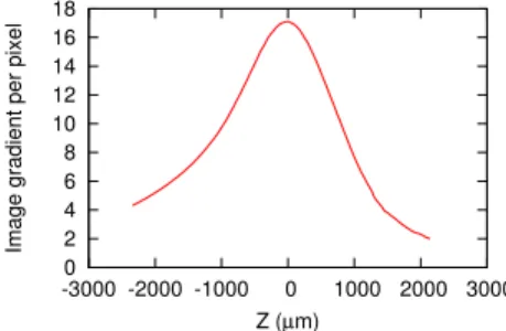
17.20-S-HV 2Basler acA1600-60gm 0 2 4 6 8 10 12 14 16 18 -3000 -2000 -1000 0 1000 2000 3000
Image gradient per pixel
Z (µm)
Fig. 3. Image gradient per pixel with respect to z position
image in our experiments from the digital microscope is
659⇥ 494 pixels.
B. Validation of the method
First, the positioning stage is moved from -2.3 mm to 2.1 mm along the z axis to evaluate the variation of image gradient with respect to z position. Images are acquired at each 40 µm step. By computing the image gradient per pixel for each image, the relation between the image gradient and z position is shown in Fig. 3. It can be seen from the figure that the depth of field is small enough for an accurate positioning and a single optimum is found in image gradient.
In positioning experiments, the stage is first set to an initial pose then moved to a predefined desired pose iteratively by comparing the image at the desired pose with the image at the current pose. The focus of microscope is adjusted so that the image is focused at the desired pose.
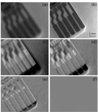
To validate the method, the initial pose of positioning stage is set to 500 µm in x and 1 mm in y axes, 2 mm in z axis; 0.1° around x axis, 2° around z axes away from the desired pose to test the performance of the proposed method. The initial image and desired image after image processing is shown in Fig. 5(a) and Fig. 5(b), respectively. Fig. 5(c) to Fig. 5(d) shows the evolution of image intensity error
eI(q) = I(q) I⇤until the end of visual servoing procedure.
The velocities converge fast to 0. As a consequence of optimization, the error image is almost null.
The experimental results are shown in Fig. 4. Since visual servoing is robust to calibration errors [24], the positioning task without explicit calibration performs also quite well. The image intensity error as well as image gradient error per pixel decrease to negligible values when the velocities converge. The object pose errors between the final pose and the desired pose reach 0.65 µm, 0.47 µm and 0.17 µm in translation along x, y, z axes; 0.027°, 0.036° and 0.003° in rotation around x, y, z axes, respectively. It can be mentioned that in Fig. 4(c), the image gradient error increases around the 70th iteration. It is mainly because the sample is too large that cannot be presented in the whole image. When the positioning stage is moving, details of the sample on the image vary, which causes the computation of image gradient to be slightly disturbed. In experiments, the proposed visual servoing scheme shows robustness to such situations.
-12 -10 -8 -6 -4 -2 0 2 4 0 50 100 150 200 250 300 -0.06 -0.05 -0.04 -0.03 -0.02 -0.01 0 0.01 0.02
Translation (mm/s) Rotation (rad/s)
iteration X Y Z θ x θ y θ z (a) -1000 -500 0 500 1000 1500 2000 0 50 100 150 200 250 300 -1 -0.5 0 0.5 1 1.5 2 Translation ( µ m) Rotation (deg) iteration X Y Z θx θy θz (b) 0 10 20 30 40 50 60 0 50 100 150 200 250 300 0 1 2 3 4 5 6 7 8
Image intensity error per pixel Image gradient error per pixel
iteration Image intensity error Image gradient error
(c) 0 100 200 300 400 -300 0 300 600 900 1200 82000 83000 84000 85000 Z / µm X / µm Y / µm Z / µm (d)
Fig. 4. 6-DoF positioning using hybrid visual servoing (a) Evolution of joint velocity (in mm/s and rad/s). (b) Evolution of object pose error (in µm/s and degree). (c) Evolution of image intensity error and image gradient error per pixel. (d) Object trajectory in camera frame
Fig. 5. Progress of 6-DoF positioning using hybrid visual servoing (a) Initial image, (b) desired image, (c) to (f) show image erroreI(q) at 1st,
16th, 82th and last iteration.
-0.5 0 0.5 1 0 100 200 300 400 500 600 700 -0.02 -0.01 0 0.01 0.02 0.03
Translation (mm/s) Rotation (rad/s)
iteration X Y Z θx θy θz
Fig. 6. Positioning using only image intensity based visual servoing: Evolution of joint velocity (in mm/s and rad/s)
-14 -12 -10 -8 -6 -4 -2 0 2 0 50 100 150 200 250 300 350-0.07 -0.06 -0.05 -0.04 -0.03 -0.02 -0.01 0 0.01
Translation (mm/s) Rotation (rad/s)
iteration X Y Z θx θy θz
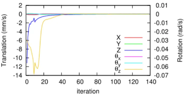
Fig. 7. Positioning using hybrid visual servoing: Evolution of joint velocity (in mm/s and rad/s)
C. Hybrid visual servoing vs visual servoing using image intensity
Experiments have been achieved to evaluate the proposed hybrid visual servoing by comparing to an approach using only image intensity [10] in the same conditions. The initial pose of the positioning stage is set to be 2 mm on z axis and 2°around z axis away from the desired pose. The positioning task based on the proposed hybrid visual servoing and image intensity based visual servoing are accomplished respectively. The evolution of joint velocity are illustrated in Fig. 6 and Fig. 7. The positioning error on translation along z axis with hybrid visual servoing is 0.26 µm, which is smaller than with the image intensity based visual servoing (1.66 µm), where also more iterations are needed to converge. On other DoFs, both these two methods perform equivalent, where the pose errors are less than 0.6 µm in translation along x and y axes, less than 0.01° in rotation around x, y and z axes. Furthermore, because of the limited travel range of the positioning stage on z axis, the initial pose on z cannot be extremely far away from the desired pose. Indeed, in that case, the image-intensity-only method fails to converge because little details can be extracted from the initial blur image. However, the hybrid visual servoing performs well since the motion on z axis can be conducted even the image is heavily blurred.
D. Robustness to light variation
As the proposed method uses photometric information, the sensibility to variable light conditions is indeed an important issue. Therefore, the robustness to light variation of the proposed method is tested. The initial pose of the stage is also set to be 2 mm on z axis and 2° around z axis. Fig. 8 shows the evolution of joint velocity. The luminance
-14 -12 -10 -8 -6 -4 -2 0 2 0 20 40 60 80 100 120 140 -0.07 -0.06 -0.05 -0.04 -0.03 -0.02 -0.01 0 0.01
Translation (mm/s) Rotation (rad/s)
iteration X Y Z θ x θ y θ z
Fig. 8. Positioning using hybrid visual servoing with lightning perturbation: Evolution of joint velocities (in mm/s and rad/s)
of the environment light is changed suddenly at the 8th iteration. Oscillations in velocities appear, caused by the lighting changes. However, the convergence and the accuracy are unaffected in spite of the changing light. The system keeps stable for a small perturbation occurring during the positioning task.
V. CONCLUSION
In this paper, a hybrid visual servoing scheme is pro-posed for an accurate and robust 6-DoF micropositioning. Differently from traditional visual tracking and object local-ization approach, only pure image photometric information is needed in this method. The image intensity information is employed to control the linear motion along x, y axes and the angular motion around x, y, z axes. To improve the precision of positioning on z axis, image gradient is introduced as a new visual feature according to the variation of image sharpness due to the motion along z axis. This method is validated by experiments on a 6-DoF parallel positioning stage and a digital microscope. Although the initial pose is far away from the desired pose (2 mm in translation and 2° in rotation), the results are accurate (pose errors are below 1 µm in translation, below 0.04° in rotation around x, y and 0.003° in rotation around z). Future work will be to modify the sensor projection model and to validate this approach with a scanning electron microscope.
ACKNOWLEDGMENT
The authors would like to thank Soukeyna Bouchebout, Mokrane Boudaoud and Jean Ochin Abrahamians for their help during the experiments at ISIR, Universit´e Pierre et Marie Curie. The positioning stage is supported by French Robotex platform. This work was realized in the context of the French ANR P2N Nanorobust project (ANR-11-NANO-0006).
REFERENCES
[1] C. Pawashe and M. Sitti, “Two-dimensional vision-based autonomous microparticle manipulation using a nanoprobe,” J. Micromechatronics, vol. 3, pp. 285–306, July 2006.
[2] S. Fatikow, C. Dahmen, T. Wortmann, and R. Tunnell, “Visual feedback methods for nanohandling automation,” I. J. Information Acquisition, vol. 6, no. 3, pp. 159–169, 2009.
[3] S. Devasia, E. Eleftheriou, and S. Moheimani, “A survey of control issues in nanopositioning,” Control Systems Technology, IEEE Trans-actions on, vol. 15, no. 5, pp. 802–823, 2007.
[4] N. Ouarti, B. Sauvet, S. Haliyo, and S. R´egnier, “Robposit, a robust pose estimator for operator controlled nanomanipulation,” Journal of Micro-Bio Robotics, vol. 8, no. 2, pp. 73–82, 2013.
[5] Y. Sun, M. Greminger, D. Potasek, and B. Nelson, “A visually servoed mems manipulator,” in Experimental Robotics VIII. Springer, 2003, pp. 255–264.
[6] N. Ogawa, H. Oku, K. Hashimoto, and M. Ishikawa, “Microrobotic visual control of motile cells using high-speed tracking system,” Robotics, IEEE Transactions on, vol. 21, no. 4, pp. 704–712, 2005. [7] C. Collewet, E. Marchand, and F. Chaumette, “Visual servoing set
free from image processing,” in IEEE Int. Conf. on Robotics and Automation, ICRA’08, Pasadena, CA, May 2008, pp. 81–86. [8] C. Collewet and E. Marchand, “Photometric visual servoing,” IEEE
Trans. on Robotics, vol. 27, no. 4, pp. 828–834, August 2011. [9] B. Tamadazte, N. Le-Fort Piat, and E. Marchand, “A direct
vi-sual servoing scheme for automatic nanopositioning,” Mechatronics, IEEE/ASME Transactions on, vol. 17, no. 4, pp. 728–736, 2012. [10] L. Cui, E. Marchand, S. Haliyo, and S. R´egnier, “6-dof automatic
micropositioning using photometric information,” in IEEE/ASME Int Conf. on Advanced Intelligent Mechatronics, AIM’14, 2014. [11] L. Cui and E. Marchand, “Calibration of scanning electron microscope
using a multi-images non-linear minimization process.” in IEEE Int. Conf. on Robotics and Automation, ICRA’14, 2014.
[12] J.-L. Pouchou, D. Boivin, P. Beauchłne, G. L. Besnerais, and F. Vi-gnon, “3d reconstruction of rough surfaces by sem stereo imaging,” Microchimica Acta, vol. 139, no. 1-4, pp. 135–144, 2002.
[13] S. K. Nayar and Y. Nakagawa, “Shape from focus,” Pattern analysis and machine intelligence, IEEE Transactions on, vol. 16, no. 8, pp. 824–831, 1994.
[14] A. P. Pentland, “A new sense for depth of field,” Pattern Analysis and Machine Intelligence, IEEE Transactions on, no. 4, pp. 523–531, 1987.
[15] P. Favaro, A. Mennucci, and S. Soatto, “Observing shape from defocused images,” Internat. J. Comput. Vision,, vol. 52, no. 1, pp. 25–43, 2003.
[16] S. Bhasin and S. Chaudhuri, “Depth from defocus in presence of partial self occlusion,” in Computer Vision, 2001. ICCV 2001. Pro-ceedings. Eighth IEEE International Conference on, vol. 1, 2001, pp. 488–493 vol.1.
[17] D. Ziou and F. Deschenes, “Depth from defocus estimation in spatial domain,” Computer Vision and Image Understanding, vol. 81, no. 2, pp. 143 – 165, 2001.
[18] F. Chaumette and S. Hutchinson, “Visual servo control, Part I: Basic approaches,” IEEE Robotics and Automation Magazine, vol. 13, no. 4, pp. 82–90, December 2006.
[19] E. Marchand and C. Collewet, “Using image gradient as a visual feature for visual servoing,” in IEEE/RSJ Int. Conf. on Intelligent Robots and Systems, IROS’10, Taipei, Taiwan, October 2010. [20] E. Marchand and N. Courty, “Controlling a camera in a virtual
environment: Visual servoing in computer animation,” The Visual Computer Journal, vol. 18, no. 1, pp. 1–19, Feb. 2002.
[21] A. Dame and E. Marchand, “Mutual information-based visual servo-ing,” IEEE Trans. on Robotics, vol. 27, no. 5, pp. 958–969, Oct. 2011. [22] B. Horn and B. Schunck, “Determining optical flow,” Artificial
Intel-ligence, vol. 17, no. 1-3, pp. 185–203, Aug. 1981.
[23] J. Ens and P. Lawrence, “An investigation of methods for determining depth from focus,” Pattern Analysis and Machine Intelligence, IEEE Transactions on, vol. 15, no. 2, pp. 97–108, 1993.
[24] B. Espiau, “Effect of camera calibration errors on visual servoing in robotics,” in Int. Symposium on experimental Robotics, ISER’93, Kyoto, 1993.