FLUVIAL THERMAL
REGIME PREDICTION
TWO-DIMENSIONAL DEPTH A VERAGED FLUVIAL THERMAL
REGIME PREDICTION
Mourad Heniche, Yves Secretan, Jean Morin, Jean-François Cantin & Michel Leclerc
Institut National de la Recherche Scientifique, lNRS-ETE Québec (Québec), Canada
GIK9A9
Rapport de recherche N° R-859
Équipe de réalisation
Institut National de la Recherche Scientifique - Eau, Terre et Environnement (INRS-ETE), 490 rue de la Couronne, Québec, QC, Canada GIK 9A9
Mourad Heniche Yves Secretan Michel Leclerc
Environnement Canada, Service Météorologique du Canada, Sainte-Foy, QC, Canada G 1 V 4H5
Jean Morin
Jean-François Cantin
Pour les fins de citation:
Heniche M., Secretan Y., Morin J., Cantin J.-F. & Leclerc M.
Two-Dimensional Depth Averaged Fluvial Thermal Regime Prediction. Rapport INRS-ETE R-859, 33 pages.
M.HENICHE, Y.SECRETAN, 1. MORIN, J.-F. CANTIN and M. LECLERC
Abstract
River temperature prediction is an important tool for environmental impact assessment as temperature is a key control factor in numerous water quality processes and for the aquatic life. When the spatial distribution becomes important it is no more possible to use ID models and one has resort to 2D horizontal models.
We present here a 2D finite e1ement model for the fluvial thermal prediction. The coupling with the hydraulics is explicit which, associated to a careful choice of the formulation for the components of the thermal budget, allows to derive a linear system, numerically very efficient. The spatial discretisation is on an unstructured grid with triangular linear elements, a scheme very well suited to natural water courses.
The most significant features of the model are presented together with a steady state test case on the St-Lawrence River between Montréal and Trois-Rivières to verify the ability of the modei to represent the spatial temperature variability.
Key Words: Water temperature; Heat transfer; Transport-Diffusion, Two-dimensional model; Finite element method; Ecohydraulics; St. Lawrence River.
Introduction
Climatic changes have been lately retaining the attention of many researchers, because of their worldwide impacts, One of them is the change in river thermal regime. Urban, land and industry usages, thermal power plants, reservoir releases, fluvial navigation and c1imatic changes are often cited among the causes of river thermal alterations. Thermal alteration may have many critical repercussions on the fluvial environment, such as loss or even disappearance of aquatic habitats, proliferation of floating algae, deleterious modifications of the chemical and physical water properties, loss of recreational and domestic uses. In northern regions, water temperature increase during the winter season may induce an alteration of the mechanical properties of ice cover, which may in turn cause earlier ice break-up and the formation ofice jams.
Water temperature is also a crucial environmental factor for aquatic life. Directly, it acts on fishes by modulating their metabolic, physiological and behavioural activities (Wootton, 1998). Indirectly, it modifies environmental characteristics of the habitat, gas dissolution, density and surface tension (Wetzel 2001). Water temperature is considered as a dominant factor for recruitment variability in fish, especially for those species spawning on the floodplain during early spring (Koonce et al. 1977; Fortin et al. 1982). For the St-Lawrence River, the size and shape of the floodplains and flats create lateral stratification of water temperature between the main channel and the shallow nearshore zones which cannot be represented by a ID model. A 2D temperature model will for example help manage water level for protecting fish spawning areas.
Modeling the temperature consist in establishing the heat budget over the water colurnn, induding all heat sources and sinks in the exchanges with the atmosphere and the riverbed. Meteorological conditions play an important role as solar and atmospheric radiations, evaporation, surface and riverbed convection and precipitation are the main factors controlling water temperature. When the flow inertia is important, it becomes essential to consider the effects of flow velo city and turbulence.
Many researchers developed ID horizontal models, assuming a constant temperature over the whole hydraulic cross section. These models are either uncoupled from hydrodynamics (Paily
et al., 1976; Brown and Bamwell, 1987), or fully coupled (Brocard and Harleman, 1976; Bowles et al., 1977). A wide variety of models can be found, among others CHARIMA (University of
Iowa, USA, 1990), CEQUEAU (INRS-Eau, Canada, 1986), DSTEMP (Utah Water Research Lab., USA, 1977), MIKEll (DHI, Denmark), MNSTREM (University of Minnesota, USA, 1994), QUAL2E and QUAL2E-UNCAS (EPA, USA, 1986) and SNTEMP and SSTEMP (US Geological Survey, USA, 2000). For lakes, where one has to take into account vertical stratification, ID vertical models were first used (Hondzo and Stefan, 1991, Stefan and Hondzo, 1998). In their part, Ahsan and Blumberg (1999) propose a 3D finite-difference model on orthogonal body-fitted grid. For estuaries, researchers often use 2D vertical models, while the first use of 2D horizontal model for ocean temperature simulation can be traced back to the work of Rosati and Miyakoda (1988). For rivers, 2D models appear to be less used. Hankin et al.
M.HENICHE, Y.SECRETAN, J. MORIN, J.-F. CANTIN and M. LECLERC
(2001) present an example of a finite volume model exploiting the hydraulics simulated with the finite element model TELEMAC-2D (EDF-LNHE, France, 2001).
As for the present work, the context is one of modeling the spatial temperature distribution of rivers like the St-Lawrence River with large flats, small channels, fluvial lakes, etc. The hypothesis for a 2D horizontal model are holding and there is no stratification. The response time of the hydraulic system is rather slow, even more as the St-Lawrence River is regulated. On the other side, temperature has a much shorter time step. It is therefore possible and advantageous to decouple the temperature simulations from the hydrodynamic simulations.
The main objective of this paper is to present a 2D horizontal finite element model to predict depth averaged water temperature in rivers, while the hydrodynamic is uncoupled. This model enhances a series of finite element models such as MODELEUR (DTM), HYDROSIM (hydrodynamics) and DISPERSIM (transport-diffusion, water quality), developed during the last decade and mainly used for eco-hydraulics studies (Secretan and Leclerc 1998, Heniche et al.
2000, Secretan et al. 2000).
This contribution is organized in five sections. The first one presents the conceptual model used to establish the thermal budget over the water colurnn. The second section introduces the 2D transport-diffusion mathematical model to predict water temperature, with the heat sources and sinks presented in the previous section. The third section focuses on the numerical implementation with an emphasis on data management. In the fourth and the fifth sections, the developed model is applied to a St. Lawrence River reach located between Montréal and Trois-Rivières (Québec, Canada) in order to asses the ability to simulate the observed lateral spatial temperature distribution. Throughout the paper, the physical variables used are expressed in SI units.
Thermal budget
It is now well established that in natural streams, water temperature is mainly controlled by climatological parameters such as solar radiation, air temperature, atmospheric pressure, humidity, precipitation and wind speed, among others that will be introduced along the
presentation. The standard way to add water temperature prediction capabilities to the basic transport-diffusion partial differential equation (PDE), is to establish the thermal budget over the water column. It consists in finding out and modeling the heat sources and sinks, which will then be introduced in the goveming PDE presented in the next section.
Rence, the total heat flux S that contributes to warm or cool the water column is expressed by the following relation:
(1)
where Sa and Sb are respectively atmospheric and riverbed thermal fluxes. Reat fluxes with the atmosphere Sa normally represent the most significant contribution to the total heat budget S. It is composed of different contributions: solar radiation Hs, long wave atmosphere's and water radiations Hl, evaporation He, surface convection He and precipitation Hp:
(2)
Reat flux due to solar radiation Hs always warms the water. It depends on the net incoming solar radiation Hsi. As the expression to model Hsi can be rather complicated (Sinokrot and Stefan, 1994), we chose instead to rely on meteorological stations located close to the reach for providing measured values at least for the net heat flux at the air water interface. Rence, it is necessary to consider reduction effects due to local terrain characteristics such as bank vegetation cover and wat€r turbidity, and to give the solar radiation flux Hs the following expression:
(3)
The shading factor SF varies from 0 (no vegetation) to 1 (complete cover) (Sinokrot and Stefan, 1993). Water albedo ris equal to 0 for clear water and varies between 0.06 and 0.12 for turbid waters (Mohseni and Stefan, 1999).
Long-wave radiation Hl pIays a mixed roIe, sometime as a heat source, otherwise as a heat sink depending of the respective water and air temperatures. Its expression is being given by:
M.HENICHE, Y.SECRETAN, J. MORIN, J.-F. CANTIN and M. LECLERC
(4)
where o=5.67051xl0-8W.m-2.K-4 is the Stefan-Boltzman constant, &w=0.97 is the water emissivity. Atmospheric emissivity Ba can be expressed as Ba =Bac(1+0.17C;). According to Swinbank (Brocard and Harleman, 1976), atmospheric emissivity for clear sky Bac may be approximated by Bac
=
0.937 xl 0-5 (273.15+
Ta)2. Cloudiness parameter Cc, varies between 0 and 1, corresponding respectively to clear and completely overcast sky. Variation of Ba is in the interval 0.75 to 1.0 for practical temperature range.Heat flux He resuIting from evaporation contributes to cool the water column. In the literature, one generally find that a Dalton law is used to model He. It combines a wind function f(Wz) to the difference in vapour pressure between saturated vapour pressure es and vapour pressure ea at air temperature Ta to give:
(5)
Numerous formulas exist to represent the wind function f(W). In this study, we have chosen the formula proposed by Marciano and Harbeck (Brocard and Harleman, 1976) because it does not only yield resuIts similar to other formulas proposed in the literature, but it only requires as input data the wind velocity
Wz
measured at 2 m (z=2) above water surface, f(W2)=
3.9 x 10⁻² W2 •Saturated vapour pressure es can be precisely estimated by the Magnus-Tetton formula (Sinokrot and Stefan, 1994) es (Pa) = 610.78 exp[(17.26939Ta )/(Ta
+
237.29)], whereas vapour pressure ea atair temperature is related to saturated vapour pressure via relative humidity RH in percents (%),
ea
=
(RH 1100) es .Heat flux He due to convection at the water surface is estimated by the Bowen law (Bowen 1926) expressed as:
where R denotes the Bowen coefficient, R=6.1x10⁻⁴Patm(T-TJ/(es-eJ and Patm the atmospheric pressure.
Heat flux Hp due to precipitation must take into account both rain and snow faU. A heat
transfer law is retained to express the heat exchange taking place at air-water interface due to rainfall. We write:
(7)
where Pr and cp denote respectively the rain precipitation, in mass rate per unit of area, and the specific heat of water. The expression for heat ex change due to snow precipitation inc1udes three physical phenomenon: heat ex change in solid phase until melting temperature is reached, energy to change phase from solid to liquid and heat exchange in liquid phase. This process is represented by:
(8)
where ps, cpù Li and Tm represent respectively the precipitation of snow, in mass per unit of area,
the specific heat of ice, the latent heat of ice melt and the snow melting-point temperature. Notice that the impact on hydrodynamics of the extra volume of water due to precipitation is not taken into account as it is considered to be negligible in comparison to the flow.
Heat exchanges with the riverbed Sb can become quite important, especiaUy when shallow
waters are considered, combined with small time steps such as hourly prediction (Brown, 1969; Jobson, 1977; Sinokrot and Stefan, 1994). In practice, the determination of Sb is quite difficult.
As the underground temperature can be considered constant, a thermal conduction law is employed to express the riverbed heat exchange:
(9)
where Kb and Tb are respectively riverbed interface heat exchange coefficient and riverbed temperature. Other techniques to estimate Sb are also available and the reader is referred to
M.HENICHE, Y.SECRETAN, J. MORIN, J.-F. CANTIN and M. LECLERC
Mathematical model
The 2D depth averaged transport-diffusive equation is retained to predict the transient temperature. Assuming steady state hydrodynamic conditions, the goveming partial differential equation in non conservation form is given by:
or
oT
or
0oT
oT
0oT
oT
h-+h(u-+v-)--h(D -+D -)--h(D -+D - ) +ot
ox
Dyox
xxox
xy Dy Dy yxox
.w Dy oS
Qh(T-T
) - - = 0 (10) pepwhere t and (x,y) are respective1y time and Cartesian coordinates; T, the depth-averaged temperature; h is the water depth; u and v are the components of the depth-averaged flow velo city vector U; Q is the groundwater and/or tributary thermal discharge per volume unit, injected if
Q
is positive, or abstracted if negative, and Ta it's corresponding temperature. In the last term of equation (10), S, p and cp stand for the heat budget as presented in the previous section, the water density and specific heat capacity ofwater, respectively.The determination of the turbulent diffusion coefficients D:xx, Dyy, Dxy=Dyx lS made
according to the following relationships (Bédard, 1997):
(11)
where
e
is the direction of the flow velo city; DL and DT correspond to the longitudinal and transversal diffusion. These are in tum expressed as a linear combination of vertical (Dv),horizontal (DH) and molecular (DM) dispersion coefficients:
The weighting coefficients
Pv, PH
andPL
are determined during the calibration procedure as to best-fit predictions with measures. The hydrodynamic 2D shallow water model provides values for Dv and DH because they depend upon the flow characteristics. Following Fisher et al. (1979), Dv can be estimated by a Taylor law, Dv=
K Dv u.H , where u. is the shear velocity; K Dv is aconstant which can vary between 0.135 and 0.17, 0.15 being the most commonly employed value. In the horizontal direction, DH takes the expression of the eddy viscosity from the
turbulence model, here a "mixing length" c1osure, D H
=
l~
2( éù)2+
2( av)2+
(éù+
av)2 where &cY
cY
&lm is the mixing length value used for the hydrodynamic simulation.
To solve equation (10) in time, boundary as well as initial conditions must be prescribed. On an inflow boundary, one has to specify the temperature as a function of time. On an outflow boundary, one has to prescribe a free exit condition. More details on boundary conditions schemes for transport-diffusion phenomenon in rivers can be found in Padilla et al. (1997). In addition, according to the drying-wetting capabilities of the hydrodynamic model, situations may occur where one has either wet or dry areas. For the dry areas, the depth is set to zero and the temperature is assumed zero.
Numericallmplementation
The transport-diffusion with thermal source/sink term (10) is solved with respect to water temperature. The Galerkin finite e1ement (FE) method is employed to achieve this goal. A 3-nodes triangular element is used to discretize the goveming partial differential equation with a linear approximation of the temperature (Pl approximation) (Secretan et al., 2000). The well-known wiggles that may appear in the solution of transport-diffusion equation are controlled through local mesh refinement andlor by tuning the diffusion coefficients. The time derivative is approximated by a stable first order Implicit Euler scheme, or a less stable but more accurate second order Crank-Nicholson scheme. In practice, the choice of a given scheme depends upon the physical particularities of the problem under study.
M.HENICHE, Y.SECRETAN, J. MORIN, J.-F. CANTIN and M. LECLERC
The resulting algebraic system, which arises from the FE discretisation, may be linear or non-linear in T depending on the expression of the thermal budget S because aIl other terms in (10) are linear in T. Obviously, a linear system in T is preferable to reduce the computational costs (Bowles et al., 1977) and to allow transient simulations in reasonable computer time.
Regrouping the expressions for the different heat source and sink terms, one can write the global thermal budget S as S
=
a(t)T + b(t) where a(t) and b(t) are transient coefficients thatdepend on meteorological data. To obtain a linear model in T, three conditions must be satisfied: physical properties of water such as density p and specifie heat cp must be kept constant; the wind function f(W) in (5) must be independent from T; finally the term in T 4 in the long-wave radiation equation (4) must be approximated through a linear regression (Mohseni and Stefan, 1999), 0"8w(273.15 + T)4 "'" 0"8wCAlT + BI) (14). Over the water temperature interval 0::; T(oC)::; 50 , the linear regression coefficients are as follows: AF1.06545x108°K3 and B[=5.37180x10⁹°K4 with a corresponding correlation of 0.9951. Note that an even better fit may be obtained by reducing the temperature interval.
Another important aspect related to the numerical implementation is the data structure. From section 2, it is manifest that the amount of data needed to feed the sub-models for the different heat sources and sinks is enormous. By judicious choices, we reduced the volume of data to a 'manageable size, while keeping the numerical tool as open as possible to implement new formulae for the sub-models.
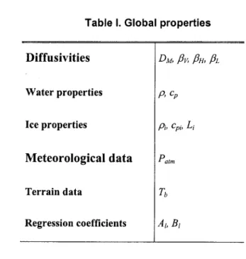
GeneraIly, one may distinguish between global and nodal properties. A global property is assumed to be constant in time and space over the entire computational domain. A nodal property is variable both in time and space, assuming a different value at each node for each time step. It is c1ear that nodal properties are much more memory consuming, especially for transient simulations. Thus, as much as possible, a maximum of physical data have been transferred to global properties.
Table 1 lists the 13 global properties that have been selected. The atmospheric pressure was introduced as a global property according to Sinokrot and Stefan (1994) who found that its
vari abi lit y has a weak influence on water temperature. As mentioned by Brown (1969), bed substrate is the most important factor in the heat transfer at water-riverbed interface. So, we retained riverbed temperature Tb as a global property and Kb as a nodal property that is less
tedious to determine through a field campaign.
Table II lists the 14 nodal properties selected, formed of 3 terrain variables, 5 hydrodynamic simulation results and 9 meteorological input data. The set of terrain data contains water-riverbed heat transfer coefficient Kb, shading factor SF and water albedo r. The
hydrodynamic data set contains the velocity components u and v, water depth h and the dispersion coefficients DH and Dv. The set of meteorological data and the corresponding
parameters contains solar radiation Hsi, air temperature Ta, air emissivity Ba, relative humidity RH, wind function f(1f'z), precipitation of rain pr if Ta ;::: O°C or snow ps if Ta < O°C. One may note that such an organization of input data enables to choose altemate expressions of Ba, f(1f'z),
and Kb depending on the user's preferences. For example, Paily et al. (1976) have found more
than 60 formulas for f(Wz) in the literature.
This model was implemented in DIS PERS lM, a FORTRAN finite element code dedicated to water quality modeling (Secretan et al., 2000). The linear system is solved with a LU
factorization method exploiting the sparse structure of the matrix. More than 30 test cases where elaborated and routinely run to assert the correctness of the code, more or less term by term. These tests are not reported here.
Study Reach : St.-Lawrence River
The objective of this application is principally to verify the ability of the model to predict the transverse variation of temperature. It is simple to establish a priori that the regions that will be thermically more active are the shallow regions with small velocities. Therefore, one of the legitimate question concems the accuracy of the numerical terrain model, the quality of the hydraulics and finally the response of the temperature model which depends on the other two models.
M.HENICHE, Y.SECRETAN, J. MORIN, J.-F. CANTIN and M. LECLERC
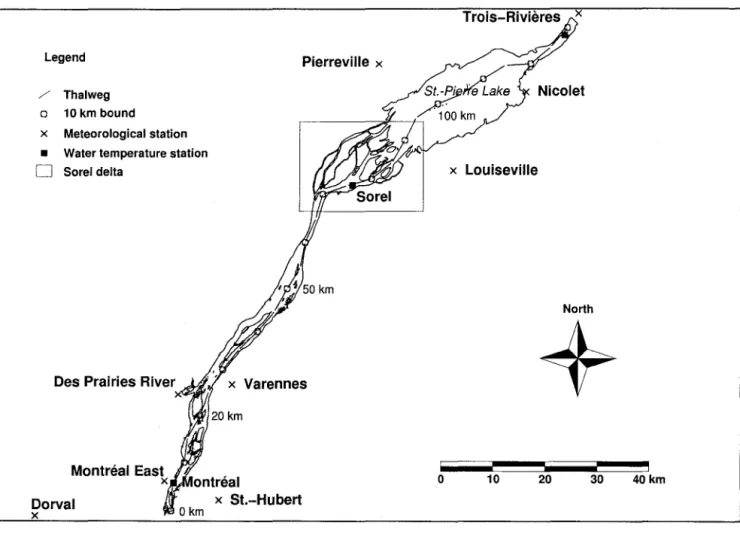
The study reach is presented on Fig. 1. The length of the computational domain stands around 130 km between Montréal and Trois-Rivières. Three important cities are located along this reach, Montréal upstream, Sorel in the middle and Trois-Rivières downstream, as well as half of Quebec's population and important industrial activities. The river is straight between Montréal and Sorel. Rowever, several islands contribute to make the reach fairly complex. In the Sorel region, a breaded network expands over 20 km and forms a large delta. Further downstream, Lake St. Pierre, a 50 km long fluvial enlargement of the river, closes the study reach. Even if this section is called lake, it has nothing to do with lacustrial behaviour, given its shallow depth and its huge discharge which stands around 9500 m3/s. Excluding Lake St.-Pierre, the average width is about 2.5 km. Several tributaries contribute to the flow, the most important being Des Prairies River on the upstream part. The Montréal urban community wastewater contributes a significant thermal release. The flow is strongly regulated with about 50 to 70% of the discharge flowing through the navigation channel that has 12 m as minimum depth and 250 m as minimum width. The flow regime is sub-critical and the average velo city varies roughly between 0.5 to 1.5 mis.
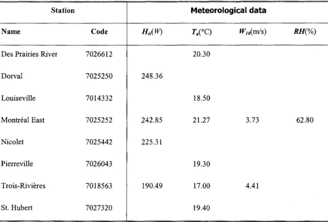
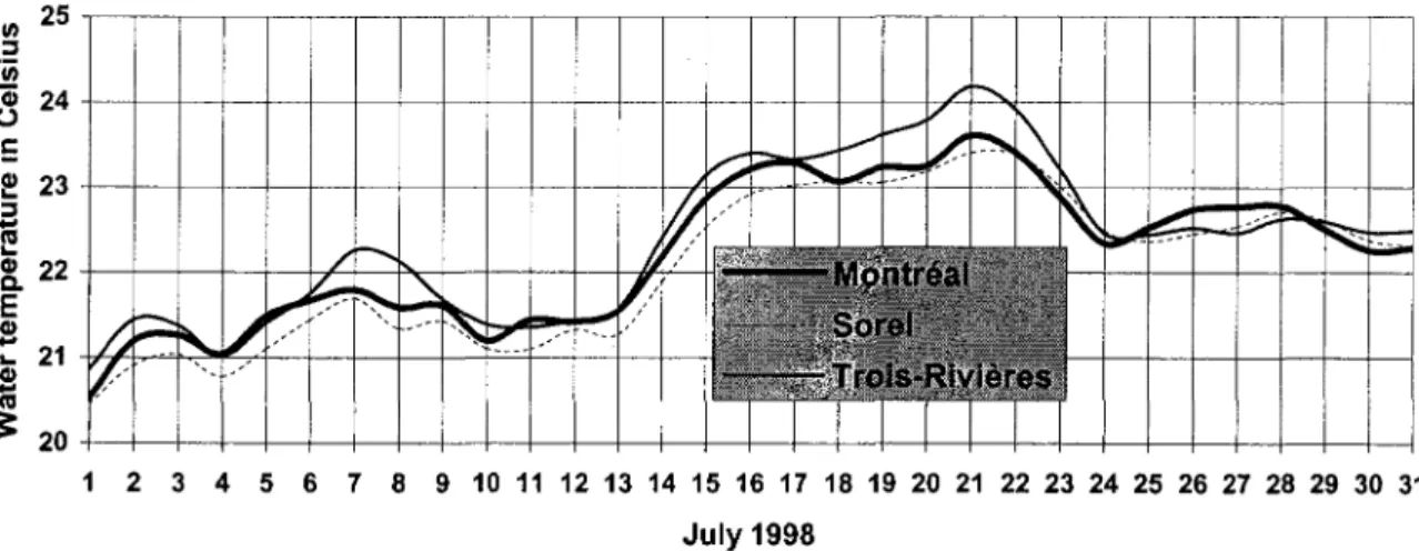
Triboulet et al. (1977) established that two to three days in average are required for water to travel across this reach. Renee, if over a typical period of one week, the observed daily water temperature remain fairly constant, one may assume steady state conditions. The present study is based on three hourly water temperature measurement stations managed by Fisheries and Oceans Canada. They are located at Montréal, Sorel and Trois-Rivières along the navigation channel (Fig. 1). Fig. 2 presents the daily averaged water temperature values for July 1998 where portions exhibit steady state conditions. July 27, 1998 was retained as the reference period because all the data required to run the model were available for that day. On the region of interest and for the period retained, 9 climatological stations provided hourly data and/or daily average data (Fig. 1). The hourly data stations provided solar radiation, wind velocity and relative humidity. The daily average data stations provided air temperature and precipitation (Table ID).
As Montréal East is the only station with recorded relative humidity data for that day, we imposed a constant value of relative humidity RH=62.80% on the whole computational domain. Air temperature varies from 17°C in the northem area near Trois-Rivières, to 21.3°C, in the
southem area at Montréal East. Rain precipitation was neglected. Solar radiation varies from 190.5W north to 248.4W south. Wind velocity WJO is in the interval of3.7 to 4.4
mis
measured at 10 m above the ground. In order to use the wind function f(Wz), the wind velocity WJO was converted into W2, Wz=
~o ln (2/ Zo )/ln(l 0/ zo), an expression derived from boundary layer theory where, according to Brutsaert (Mohseni and Stefan,Zo
=
10x exp(1O-3 K(l +0.07~ot1l2)
and where l(= 0.4 is the Von Karman's constant.2000),
To complete the input data, the shading effect of bank vegetation was neglected (SF=O) considering the width of the stream, and water was assumed to be clear (r=0). The following global physical parameters were used: p=1000kg.m-3, cp=4181.6 J.kg-1.0C-1, Patm=101080Pa,
Tb=O°C and DAF10-6m2.s-1•
Results
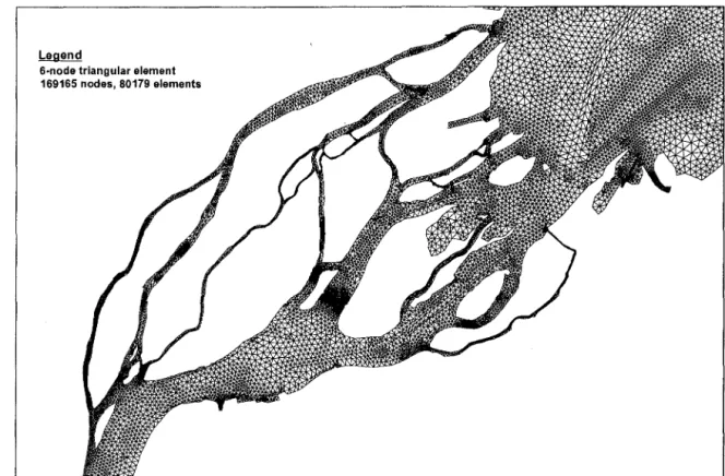
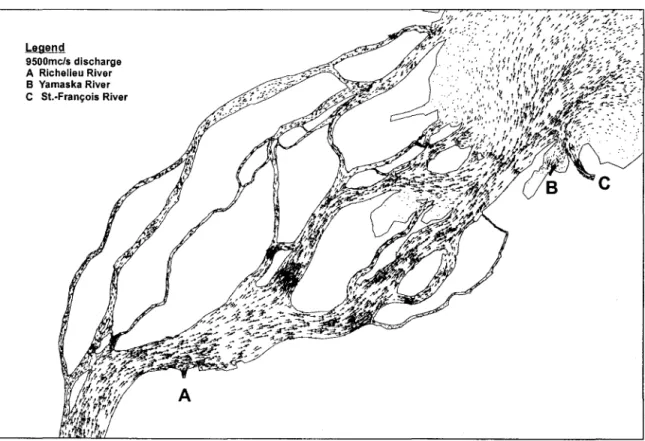
The mesh used to perform the computation counts 169165 nodes and 320716 linear triangular elements (3-nodes, Pl approximation). It was obtained by splitting in four each (6-nodes, P11P1 isoP2) triangular elements of the mesh used for the hydrodynamic simulations (Fig. 3), thus conserving the topology of the hydrodynamic mesh. Terrain data interpolation, mesh generation and hydrodynamic simulation were done with the software package MODELEUR-HYDROSIM (Secretan and Leclerc, 1998; Heniche et al., 2000). The hydrodynamic scenario retained corresponds to the mean annual discharge of 9500 m3/s a representative value of the flow discharge for this period. The hydrodynamic complexity is particularly visible in Fig. 4, underlining the usefulness of a 2D model.
The mean values for horizontal and vertical diffusivities as generated by the hydrodynamic mode1 are about 0.039 and 0.014m2/s respectively. The parameters diffusion Pr10-2, PFFl.O and
PL=105 were set considering two main criterions. In rivers, according to Fisher (reported by Brocard and Harleman, 1976), horizontal turbulent diffusion is generally several times more important than vertical. The longitudinal diffusion was set to best fit the measures as well as to reproduce at best the temperature plumes. It is well established that on the St. Lawrence River mixing between tributary waters flowing along the banks and the main channel is poor over long
M.HENICHE, Y'sECRETAN, J. MORlN, J.-F. CANTIN and M. LECLERC
distances (several tens of km). In a previous study undertaken between Montréal and Québec City, Triboulet et al. (1977) measured water temperature variations up to 12°C between banks. The parameters where also set to produce a smooth solution and control the wiggles.
Boundary conditions are prescribed at Montréal Harbour and Des Prairies River where the temperature was fixed according to measurements. Hence, at Montréal Harbour, Dirichlet boundary conditions are imposed on temperature with a value of 22.74 oC. This value is equal to the one observed at Montréal navigation channel station. It was assumed to be of equal magnitude because of the proximity between the two sites. At Des Prairies River, the temperature measured by the Urban Community of Montréal (CUM) was T=23.6°C. At the downstrearn boundary, a condition of free exit was imposed (Padilla et al., 1997). On the other closed and inflow boundaries, a homogeneous Neumann condition was imposed. As the problem is of steady state type, no initial condition is required.
The model was calibrated with the 3 measurement points at Montréal, Sorel and Trois-Rivières. The temperatures were recorded at a short distance below the water surface. As the depth is shallow and water is weIl mixed in the vertical direction, they were assumed to be equivalent to depth averaged values. Furthermore, according to observation made by Triboulet et al. (1977), vertical variation does not exceed O.5°C. Measured water temperatures were also considered representative of steady state conditions because only small variations were observed in the meteorological data, allowing the establishment of reasonably invariant thermal conditions.
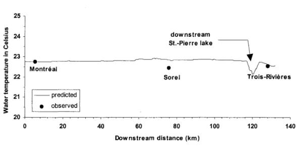
The results obtained are presented on graphs, tables as well as on maps. The values of computed water temperature versus observed ones are presented on a length profile along the navigation channel (Fig. 5). The results are in rather good agreement, the maximum error being less than O.5°C at Sorel where the prediction slightly overestimates the measurement. In accordance with observations, the model predicts a water temperature at Trois-Rivières greater than at Sorel. The simplifications introduced can certainly explain part of these differences. The water temperature of the tributaries Richelieu, St. François and Yamaska Rivers close to the Sorel area (Fig. 4) were not available, so homogeneous Neumann boundary conditions were imposed. Moreover, the hydrodynarnic scenario was set without taking into account the friction
effect of aquatic vegetation which is important in summer. The aquatic vegetation reduces the flow velocity and mixing on the flats where present, and increases the discharge in the main channel.
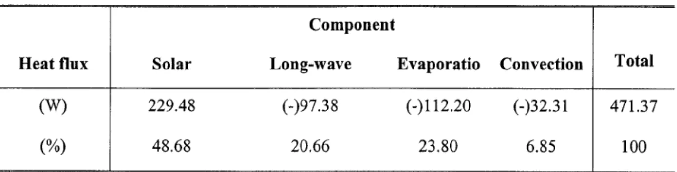
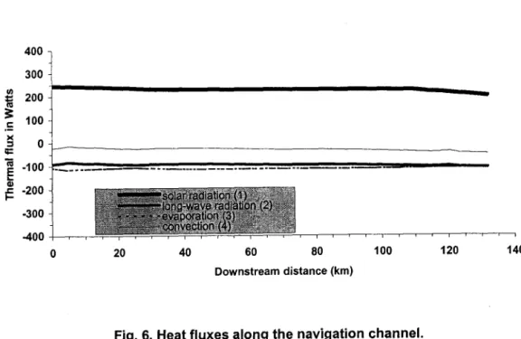
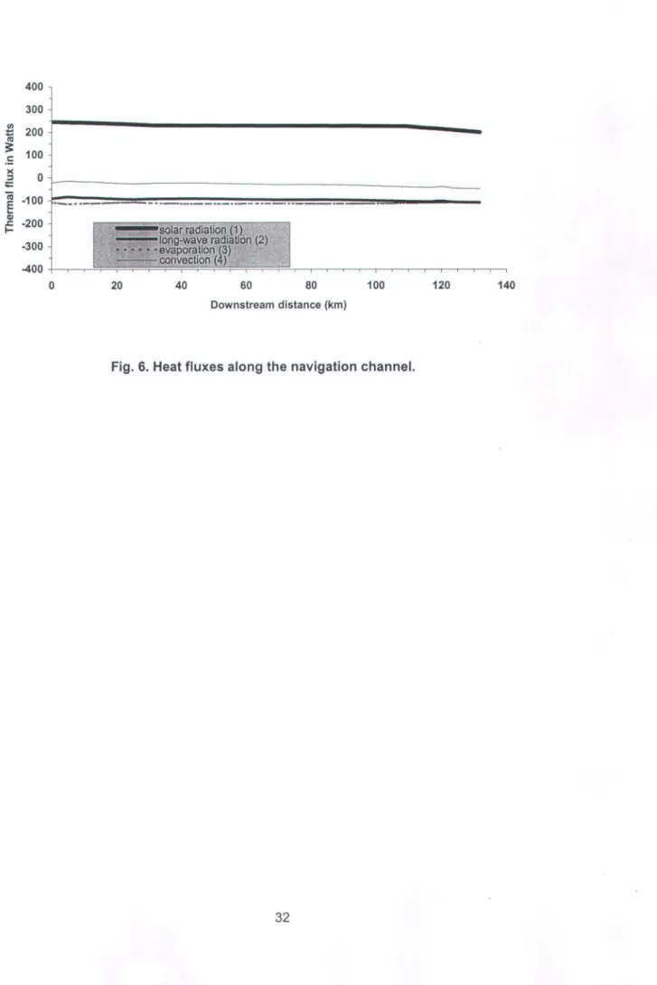
The contributions of the different components of the thermal budget along the navigation channel are presented on Fig. 6. Solar radiation is the only heat source, other components such as long-wave radiation, evaporation and convection are heat sinks. Contribution of convection flux seems to be negligible. The mean values over the domain of each component in heat budget are presented in Table IV.
Fig. 7 presents the map of the temperature distribution. The model reproduces adequately the plume on long distances as between Des Prairies River and the Sorel delta. Likewise, on Lake St.-Pierre, the model predicts an important transversal variation of temperatures with respect to mean flow. Cross sectional temperature pattern from left bank to right bank is also plotted on Fig. 7. A difference of nearly two degrees Celsius can be observed between main channel and river banks. One can also see spots of higher temperature in the shallow areas with low velocities, revealing the dynamic of these regions.
Concluding Remarks
This paper presents a 2D finite element model for river stream temperature prediction. The model has been successfully linearized, is numerically efficient and makes it possible to simulate large domains with relative ease. The data structure and software architecture retained is open and allows to choose the most appropriate experimental formulas for the sub-models that appear in several components of the thermal budget. Even though the results presented herein correspond to a steady state regime in summer conditions for daily averaged predictions, the conceptual model discussed is theoretically able to generate transient simulations with smaller time steps.
The spatial dynamic is weIl represented, the model reacts as expected in shallow regions. As these regions are the most interesting for the aquatic life, the quality of the results will greatly depend on the quality of the numerical terrain model including aquatic plant description for their
M.HENICHE, Y.SECRETAN, J. MORlN, J.-F. CANTIN and M. LECLERC
impact on the friction coefficient, and on the quality of the hydrodynamics. The task to mn the 2D temperature model is more one of data management (terrain, hydrodynamics, meteorology) because 14 values per computational no de are required for each time step. The processes of spatial and temporal input data homogenization is at best tedious.
Our primary goal here was to asses the ability of a 2D model to predict the spatial temperature variation and to evaluate the requirements such a model places on upstream data . The ultimate objective is to simulate the transient temperature signal over long periods on the St-Lawrence River. For this, we now know that we need a very accurate and very dense numerical terrain model, very precise hydrodynamics and very fine temperature data in shallow regions.
Acknowledgement
This research work was accomplished under a contract from Environment Canada. Special thanks to Patrice Fortin and Karine Legault, from Environment Canada, and Jimmy Siles, from Fisheries and Ocean Canada for their help in data collection.
APPEND~.REFERENCES
Ahsan, A.K.M.Q. and Blumberg, A.F. (1999). "Three-Dimensional Hydrothermal model of Onandaga Lake, New-York". J Hyd. Eng., 125(9),912-923.
Bédard, S. (1997). "Développement d'un modèle de transport-diffusion applicable aux rejets urbains de temps de pluie". Master Thesis, INRS-Eau, 191 pages.
Bowen, LS. (1926) "The ratio of heat losses by conduction and by evaporation from any water surface". Phys. Rev. Ser., 2(27), 779-787.
Bowles, D.S., Fread, D.L. and Grenney, W.J. (1977). "Coupled dynamic streamflow-temperature models". J Hydrau!. Div. Am. Soc. Civ. Eng., 103(5),515-530.
Brocard, D.N. and Harleman, D.R.F. (1976). "One-dimensional temperature predictions III
unsteady flows". J Hydraul. Div. Am. Soc. Civ. Eng., 102(3),227-240.
Brown, G.W. (1969). "Predicting temperatures of small streams". Wat. Res. Res., 5(1), 68-75.
Brown, L.C. and Barnwell, T.O. (1987). "The enhanced stream water quality model QUAL2E and QUAL2E-UNCAS : documentation and user manual". Environmental Research, Office of Research and Development, U.S. Environmental Protection Agency (EPA), Athens, Georgia.
Fisher, H.B., List, E.J., Koh, R.C.Y., Imberger, J. and Brooks, N.H. (1979). "Mixing in inland and coastal waters". Academic Press.
Fortin, R., Dumont, P., Fournier, H., Cadieux, C. and Villeneuve, D. (1982). "Reproduction et force des classes d'âge du Grand Brochet (Esox lucius L.) dans le Haut-Richelieu et la baie Missisquoi". Cano J Zoo!. 60: 227-240.
Hankin, B.G., Holland, M.J., Beven, K.J. and Carling, P. (2002). "Computational fluid dynamics modelling of flow and energy fluxes for a natural fluvial dead zone". J Hyd. Res., 40(4),
M.HENICHE, Y.SECRETAN, J. MORIN, J.-F. CANTIN and M. LECLERC
Heniche, M., Secretan, Y., Boudreau, P. and Leclerc, M. (2000). "A two-dimensional finite element drying-wetting shallow water model for rivers and estuaries". Adv. Wat. Res., 23, 359-372.
Hondzo, M. and Stefan, H.G. (1991). "Three Case Studies of Lake Temperature and Stratification Response to Warmer Climate". Water Res. Res., 27(8), 1837-1846.
Jobson, H.E. (1977). "Bed conduction computation for thermal models". J. Hyd. Eng., 103(10), 1213-1217.
Koonce, J. K., Bagenal, T. B., Carline, R. F., Hokanson, K. E. F. and Nagiec, M. (1977). "Factors influencing year-class strength of Percids: A summary and a Model of temperature effects". J. Fish. Res. Board Cano 34: 1900-1909.
Mohseni, O. and Stefan, H.G. (1999). "Stream temperature/air temperature relationship: a physical interpretation". J. o/Hydrology, 218, 128-141.
Paily, P.P and Macagno, E.O. (1976). "Numerical prediction of thermal-regime of rivers". J. Hydraul. Div. Am. Soc. Civ. Eng., 102(3),255-274.
Padilla, F., Secretan, y. and Leclerc, M. (1997). "On open boundaries in the finite element approximation of two-dimensional advection-diffusion flows". Int. J. Num. Meth. Eng., 40(13),2493-2516.
Rosati, A. and Miyakoda, K. (1988). "A general Circulation Model for Upper Ocean Simulation". J. Phys. Oceanogr., 18, 1601-1626.
Secretan, Y., Heniche, M. and Leclerc, M. (2000). "DISPERSIM : un outil de modélisation par éléments finis de la dispersion de contaminants en milieu fluvial". Report INRS-Eau No. R558, 57 pages.
Secretan, y. and Leclerc, M. (1998). "MODELEUR: a 2D hydrodynamic GIS and simulation software". Proceedings of Hydroinformatics Conference, on the behalf of the IAHR, Copenhagen, Denmark, 425-432.
Sinokrot, B.A. and Stefan, H.G. (1993). "Stream temperature dynamics: measurements and modeling". Wat. Res. Res., 29(7), 2299-2312.
Sinokrot, B.A. and Stefan, H.G. (1994). "Stream water-temperature sensitivity to weather and bed parameters". J. Hyd. Eng., 120(6), 722-736.
Stefan, H.G., Fang, X. and Hondzo, M. (1998). "Simulated c1imate change effects on year-round water temperature in temperate zone lakes". Climatic Change, 40(3-4),547-576.
Triboulet, J.-P., Verrette, J.-L. and Llamas, J. (1977). "Température de l'eau du Saint-Laurent de Montréal à Québec". Proceedings of the 3rd National Hydrotechnical Conference, Québec, Qué., 636-655.
Wetzel, R. G. (2001). "Lymnology, lake and river ecosytems". Academic Press, Third edition. 106 pages.
Wootton, R. J. (1998). "Ecology of Te1eost fishes". Second edition. Kluwer Academic Publishers
M.HENICHE, Y.SECRETAN, J. MORIN, J.-F. CANTIN and M. LECLERC APPENDIX.NOTATION Cc DL (m2/s) DM (m2/s) DT (m2/s) h (m) HR(%) Kb (W.m-2.0 C-I) Lg (J.kg-I) Patm (Pa) R S (W.m-2) Sa (W.m-2) Sb (W.m-2) SF TCC) Ta (OC) Tb CC) Tm (OC) U (m.s-')
Wz
(m.s-1) Cp (J.kg-1.0C-1) Cp i(J.kg-'.°C-1) = = = cloud coyer;longitudinal turbulent diffusion coefficient; molecular diffusion coefficient;
transversal turbulent diffusion coefficient; water depth;
relative humidity;
riverbed-water heat transfer coefficient; latent heat of ice;
atmospheric pressure; Bowen ratio;
heat budget;
heat budget at air-water interface; heat budget at riverbed-water interface; shading factor;
depth averaged water temperature; air temperature.
riverbed temperature; melting-point temperature;
depth averaged flow velo city vector; wind velocity measured at height z;
specific heat of water; specifie heat of ice;
f(Wz) lm (m) ps (kg.m-2.s-1) (k -2 -1) pr g.m.s
Pv
PB
p (kg.m-3) (J -2 -1 K-4) (J' .m.s.e
(rad) = wind function; gravit y; mixing length; precipitation of snow; precipitation of rain; shear velocity;weighting coefficient for Dv;
weighting coefficient for DB;
weighting coefficient for DL;
time step;
extinction coefficient of the atmospheric heat fluxes; atmospheric emissivity;
water emissivity; water density;
Stefan-Boltzman constant;
M.HENICHE, Y.SECRETAN, J. MORIN, J.-F. CANTIN and M. LECLERC
Table 1. Global properties
Diffusivities
Water properties
Ice properties
Meteorological data Patm
Terrain data
Table II. Nodal properties
Terrain data Kb, SF, r
M.HENICHE, Y.SECRETAN, J. MORIN, J.-F. CANTIN and M. LECLERC
Table III. July 27,1998 daily average values extracted trom the climatological data
Station Meteorological data
Name Code Hs;{W) Tae°C) W1O(m/s) RH(%)
Des Prairies River 7026612 20.30
Dorval 7025250 248.36 Louiseville 7014332 18.50 Montréal East 7025252 242.85 21.27 3.73 62.80 Nicolet 7025442 225.31 Pierreville 7026043 19.30 Trois-Rivières 7018563 190.49 17.00 4.41 St. Hubert 7027320 19.40
Table IV. Heat flux components
Component
Heat flux Solar Long-wave Evaporatio Convection Total
(W)
229.48 (-)97.38 (-)112.20 (-)32.31 471.37Legend Pierreville x
. / Thalweg
0 10 km bound
x Meteorological station
•
Water temperature station0 Sorel delta x Louiseville
North
Des Prairies River x Varennes
Montréal East 0
x ontréal o 10 20 30 40 km
Dorval x St.-Hubert
x
~ 25'-'--'-'-'-'--'-'-'--'-~-'--~'-'-'--'-'-'--'-'-'-'--r-'-'--'-'-'--'~ ::::J i;; ~ 24~--4-~-+-+~--~+-4-~-+-+~~i--+-~-~-+-+~~~~~~-+~--~+-4-~~ (.J .5 2 3 4 5 6 7 8 9 10 11 12 13 14 15 16 17 18 19 20 21 22 23 24 25 26 27 28 29 30 31 July 1998
M.HENICHE, YSECRETAN, J. MORIN, J.-F. CANTIN and M. LECLERC
Legend
6·node triangular element 169165 nodes. 80179 elements
Legend
9500mc/s discharge A Richelieu River B Yamaska River C St.-François River
M.HENICHE, Y.SECRETAN, J. MORIN, J.-F. CANTIN and M. LECLERC 25 1/1 ::J ëii 24 downstream Gi St.-Pierre lake
~
0 .5 23 l!!.a
Montréal•
f!22 Sorel Trois -Riviè res
al 0-E al
-
... 21 - - predicted al-
ni•
observed :i: o 20 40 60 80 100 120 140 Downstream distance (km)400 300 VI 200 i ~ 100 .5 >< 0 ::1 ;;:: iü -100 E
...
QI -200 .s::. 1--300 -400 0 20 40 60 80 100 120 140 Downstream distance (km)TWO-DIMENSIONAL DEPTH A VERAGED FLUVIAL THERMAL REGIME PREDICTION 400 300
~
200]---~
.E 100 ~ 0 ;;::: ~ -100~~==~~~~====~~~~~~==~~~~~E
.. --.... ---
..
---
..
--
....
-
-
----.. ---
________ _ CI) ~ -200 -300 -400 +----,----,-o 20 'sol~r.radiati()J) (1 L IOl'lg-~ve radiatlon;(2) > evapora.tiorr(3):~4 . çonvectlon (4) .. 40 60 80 Downstream distance (km) 100Fig. 6. Heat fluxes along the navigation channel.
Legend
Water temperature (in deg. C)
24.0 23.5 23.0 22.5 22.0 21.5 21.0