Axial acoustic field along a solid-liquid fluidized bed under power ultrasound

(1)

OATAO is an open access repository that collects the work of Toulouse

researchers and makes it freely available over the web where possible

Any correspondence concerning this service should be sent

to the repository administrator:

tech-oatao@listes-diff.inp-toulouse.fr

This is an author’s version published in: http://oatao.univ-toulouse.fr/24162

To cite this version:

Grosjean, Vincent

and Julcour-Lebigue, Carine

and Louisnard, Olivier

and Barthe, Laurie

Axial acoustic field along a solid-liquid fluidized bed

under power ultrasound. (2019) Ultrasonics Sonochemistry, 56. 274-283.

ISSN 1350-4177

Official URL:

https://doi.org/10.1016/j.ultsonch.2019.04.028

(2)

Axial acoustic

ﬁeld along a solid-liquid ﬂuidized bed under power

ultrasound

V. Grosjean

a

, C. Julcour

a

, O. Louisnard

b

, L. Barthe

a,⁎ a_{Laboratoire de Génie Chimique, Université de Toulouse, CNRS, INP, UPS, Toulouse, France}

b_{Centre RAPSODEE, UMR CNRS 5302, Université de Toulouse, Ecole des Mines d’Albi, 81013 Albi Cedex 09, France}

Keywords: Sonoreactor Acoustic cavitation Hydrophone Spectral analysis Acoustic shielding Solid suspension

This work investigates the ultrasound propagation within a liquid-solidfluidized bed. The acoustic mapping of the reactor is achieved by means of a hydrophone. A spectral analysis is carried out on the measured signals to quantify the cavitation activity. The effects of several parameters on the spectral power distribution is appraised – including emitted ultrasound power, liquid superficial velocity and solid hold-up. Results show that increasing US power promotes a higher energy transfer from the driving frequency toward the broad-band noise– which is the signature of transient cavitation– and yields a stronger acoustic shielding. The presence of a flow opposite to the acoustic streaming may affect the sonoreactor behavior by sweeping the cavitation bubbles away from the ultrasonic horn. Finally the presence of millimeter sized particles significantly increases wave attenuation, presumably due to viscous losses on the one hand, and through the contribution of their surface defects to bubble nucleation on the other hand. Moreover, the influence of the solid hold-up appears to depend upon the particle material (glass or polyamide).

1. Introduction

The use of power ultrasound (US) has raised a growing interest in chemistry and chemical engineering since the 90’s and sonochemistry now covers a large range of applications[1,2]. However, the involved phenomena are of great complexity and make the efficient design of sonoreactors into a hard task. For instance several authors reported a levelling off or even a decrease of US efficiency when increasing the acoustic power [3–5]. This effect, known as “acoustic shielding”, is explained by the reduction of active cavitation zones inside the reactor. When the acoustic power is increased, the bubble cloud densifies, which increases the attenuation of the acoustic wave, thus restricting the active zones at the very vicinity of the ultrasonic horn. Knowledge about cavitation zone distribution is paramount to understand the performance of sonoreactors, provides rational designs and extrapolate sono-processes at the industrial scale.

Characterization of sonochemical reactors can be achieved through diﬀerent techniques, and an exhaustive list can be found in several reviews and books [6–8]. The most common and classic technique is calorimetry, due to its simplicity in use[9,10]. This method quantiﬁes

the acoustic power dissipated in the liquid by measuring the time-evolution of temperature in the medium. It is a global method and does not give any information about spatial distribution or level of acoustic

cavitation. Dosimetry techniques– using for instance Fricke solution, potassium iodide, nitrophenol or terephthalate– quantify the chemical activity inside the sonoreactor, based on the oxidative activity of%OH radicals formed during the collapses of cavitation bubbles[6–8,11–13]. Again they do not in general provide information about their location. Some techniques are more focused on the spatial mapping of the sonoreactors. Aluminum foil erosion gives a direct visualization of the local intensity of cavitation [14,15], but it is diﬃcult to deﬁne a

quantitative criterion from it. Sonoluminescence, or light emission by cavitation bubbles, is a well-known phenomenon that can be utilized for characterization purpose. Yasui et al. [16] describe the state of knowledge about the underlying mechanisms. With an adequate setup it is possible to observe the zones of active cavitation and to quantify their intensity via photo-multipliers[17]. Another linked technique is based on sonochemiluminescence, where acoustic cavitation bubbles produce light by the reaction between the radicals produced during their collapse and luminol added beforehand to the solution[18,19]. A third optical method is laser tomography[12]. By illuminating the re-actor with a laser sheet, bubble clouds can be visualized. This technique is easier to set-up than the two previous ones, but it doesn’t make any diﬀerence between the active bubbles and those which are not. Finally acoustic measurements by a hydrophone can eﬃciently probe sonor-eactors [20]. It usually uses piezo-electric materials (ceramics or

⁎_{Corresponding author.}

E-mail address: laurie.barthe@ensiacet.fr(L. Barthe). https://doi.org/10.1016/j.ultsonch.2019.04.028

(3)

2. Experimental setup

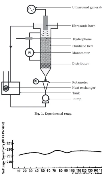
In order to investigate the behavior of power ultrasound in the presence of a solid suspension, an acoustic mapping of afluidized bed is achieved. Afluidized bed consists in an upward fluid flow (here water) that keeps solid particles into suspension by applying a drag force able to counteract the apparent particle weight. It results into a solid sus-pension whose concentration is rather uniform in the case of a liquid-solid system, without the need of a mechanical stirrer which could modify the ultrasound propagation. Solid hold-up can be then varied in a wide range by modifying the liquid superficial velocity (i.e. the ratio of the volumetricflow rate QLto the cross-sectional area of the reactor Sbed). In the present work, two types of particles are used, whose

characteristics are given inTable 1.

The reactor is made of PMMA and consists of a30cmhigh and5cm diameter wide column, comprising a liquid distributor (made of a5cm high fixed bed of 4mm diameter glass particles) at its bottom to homogenize the incomingflow and an enlargement at the top to reduce thefluid velocity. The upward liquid stream is provided by a centrifugal pump and itsflowrate (QLup to750 .L h−1) is controlled by rotameters,

thefluid circulating in a closed circuit. The temperature of the feeding tank is kept at 20 °C ± 0.5 °C. A differential manometer enables the measurement of the pressure drop between the base and the top of the fluidized bed with a precision of10Pa. Power ultrasound is emitted from an ultrasonic horn placed at the top of the column and powered by a generator. The horn/generator couple is provided by Sinaptec to get a driving frequency of20kHz. The built-in servo control prevents from working below cavitation, and frequency is tuned in a narrow range to maximize the power input in the liquid, resulting in an average value of

± kHz

19.7 0.01 . The yield of this equipment, measured by calorimetry, is around 80%. The hydrophone is introduced on the side of the column via inserts placed every centimeter to allow spatial mapping along the axis. It is not moved when varying the acoustic power or the liquidﬂow rate (without particles). The emitting surface of the ultrasonic horn lies

cm

2.5 above theﬁrst measurement point. A scheme of the experimental setup is illustrated inFig. 1.

The acoustic signal is measured by a hydrophone designed by the University of Santiago in Chile. The design of this hydrophone is de-tailed in the paper of Gaete-Garretón et al.[33]. In brief, it consists of a piezoelectric sensor encapsulated at the tip of a2mmdiameter rod. The hydrophone also includes a built-in electronic providing it with a stable sensitivity over 10–150 kHz range. It should be noticed that the sensi-tivity provided by the authors[33]was measured without the built-in ampliﬁer, hence20dBmust be added to the values given inFig. 2to obtain the actual sensitivity. The signals measured by the hydrophone are digitized by a numerical oscilloscope (PicoScope model from Pico Technology). They are then processed by a Matlab script in order to get useful information as described in the following part.

3. Acoustic signal processing 3.1. Signal processing steps

The hydrophone output-voltage U, is sampled at 18 MHz by the numerical oscilloscope in order to obtain 32 successive sequences of

Table 1

Solid particle characteristics.

Material Glass Polyamide

Diameter (mm) 2 2

Density (_{kg m}_. −3₎ 2560 1180

Speciﬁc heat (_{J kg}_. −1_._K−1₎ 753 1600

Thermal conductivity (_{Wm K}−1−1₎ 1.05 0.25

Thermal expansion coeﬃcient (_K−1₎ _4.010−6 ₈₅₁₀−6

polymers), converting their deformation by the acoustic pressure into a measurable electric signal. This will be the technique used in this work, as it provides both quantitative and local information without the need of modifying the medium of interest or the reactor, and it is thus is a good candidate as standard characterization technique for industrial set-ups.

The main pitfall of this technique is to properly interpret the mea-sured signals of acoustic pressure. Indeed the acoustic spectrum under ultrasonic cavitation displays a very rich and complex pattern. Many authors agree on the fact that the spectrum measured in a sonoreactor working at a driving frequency f₀will show lines corresponding to the

fundamental frequency ( f₀), but also its harmonics (kf₀), sub-harmonics

( f0 /n) and ultra-harmonics (kf0/n), as well as a broad-band noise

be-tween those frequency lines [20–24]. Previous works give different explanations about the genesis of those spectrum characteristics, but all agree on two points. First, if the source is strictly monochromatic, the spectrum will not show other characteristics than fundamental fre-quency unless there are bubbles in the system. Second, the spectrum lines apart from the fundamental frequency are the signature of stable (or long lifetime) cavitation bubbles. The origin of the broad-band spectrum remains an open issue. Most of the authors consider that it is directly produced by the fast collapsing or transient cavitation bubbles. Yasui et al. [25] show by numerical simulations that this broad-band spectrum is due to the fluctuation of the number of bubbles rather than to their chaotic pulsation. Yet in their conclusion, the authors state that this broad-band noise, although not directly produced by shock-waves, is strongly linked with the presence of transient cavitation, as these bubbles can disintegrate into daughter bubbles during their collapse causing the temporal fluctuation of the number of bubbles. Hence many authors define a transient cavitation index based on the quantification of this broad-band noise. One measurement method of this noise con-siders only the high frequency zone of the spectrum where no more harmonics appear. For example, Hodnett et al. [26,27] apply a band pass filter between 1, 5 MHz and 8 MHzto the signal and then define their cavitation index as the root mean square value of the resulting signal. Similarly, Uchida et al. [28,29] define the cavitation index as the integral of the spectrum over a band located in the high frequency re-gion (here between 1 MHz and 5 MHz). An alternative method is to

integrate the spectrum on a wider band, after eliminating the lines corresponding to the (sub/ultra) harmonics and/or the fundamental

[30]. This last method is more complex to apply as it needs to detect

and eliminate speciﬁc parts of the spectrum, but it is more rigorous. As said before, cavitation zone locations are very dependent on how the power ultrasound propagates inside the reactor. The main com-plexity comes from the sound attenuation due to the very presence of the cavitation bubbles (acoustic shielding). But the medium in a so-noreactor can include more than two phases (solution + bubbles), as many applications use a solid phase (lixiviation, catalytic reactions …). This added solid phase can have an impact on power ultrasound pro-pagation and thus on the location and size of active cavitation zones. The eﬀect of solid suspension on ultrasound propagation is well known in the case of diagnostic ultrasound. There are well-established models

[31,32] able to measure the features of solid suspensions (particle size distribution and hold-up) through the measurement of sound propa-gation. But this area of acoustic, known as acoustic spectroscopy, is limited to low intensity ultrasound. The behavior of power ultrasound in a solid suspension and the respective contributions of bubbles and solid to its attenuation remain mostly unknown.

To answer these issues, this work aims at investigating the propa-gation of ultrasound in a solid – liquid ﬂuidized bed, made of milli-meter-sized particles. This is achieved through an acoustic mapping of the sonoreactor with a hydrophone and an adequate processing of the measured signals. Several operating parameters are explored such as solid concentration, liquid ﬂow rate, emitted power and nature of the solid particles.

(4)

=

T 50msduration. These parameters have been found adequate from a sensitivity study (see below). Each sequence is then windowed and zero-padded before computing the fast Fourier transform. Windowing is used to reduce the amplitude of the side lobes around the peaks of the spectra, which could affect the quantification of the broad-band noise. A Hanning window is applied, which makes a good compromise be-tween the reduction of the side lobes and the increase in width of the main lobe. On the other hand, zero padding is used to enhance the spectral definition. These two steps are shown inFig. 3.

= FFT f FFT f S f ( ) ( ) ( ) p U (1) Note that the spectra are cut above 150 kHz because the sensitivity of the hydrophone is known only up to that frequency. The FFT is a complex number and only its module (| | operator) is of interest in this work. Its argument (the phase of each sinusoidal component) could not be exploited because ultrasound emission and hydrophone acquisition were not synchronized. Then the Power Spectral Density of the acoustic pressure (PSD fp( )inPa Hz2 −1) is given by the following expression[34]:

= 〈 〉 = ∫ PSD f FFT f N F W W T W t dt ( ) 2| ( )| with 1 ( ) p p sig S T 2 2 2 0 2 (2) In this expression, Nsigis the number of signal samples before zero

padding,FSis the sampling frequency, W is the window function, here

of Hanning type, and 〈W2〉 _{the period-average of its squared value} (0.375 for Hanning window). The multiplicative“2” factor arises from the symmetry property of the FFT (the considered spectra being re-stricted to the positive frequency range).

Finally the PSD is averaged over the 32 acquisitions according to:

∑

〈 〉 = = PSD ( )f 1 PSD f 32 ( ) p i p 1 32 i (3) Peaks corresponding to the (sub/ultra) harmonics and the funda-mental are extracted with the Matlab built-in peak detection algorithm. The extracted peaks are those corresponding to the driving frequencyf₀

and the (sub/ultra) harmonics multiple off₀and1f,

2 0 up to7f0which is

the last harmonics below f_max =150kHz. The width of each peak is taken as twice the full width at half maximum ( fΔ ) and their (Ppeak) is

calculated by integrating the PSD spectrum over the respective peak-width: = ∫ 〈 〉 − + Ppeak PSD ( )f df f f f f p Δ Δ peak peak peak peak (4) The total power (Ptot) is obtained from integration of the full

spec-trum up to150kHz, and the power relative to the broad-band noise (Pnoise) is deduced by subtracting that of all the peaks from the total

power: = ∫ 〈 〉 Ptot PSD ( )f df f p 0 max (5) Ultrasound generator Ultrasonic horn Fluidized bed Distributor Pump Tank Hydrophone Heat exchanger Rotameter Manometer

Fig. 1. Experimental setup.

Fig. 2. Hydrophone sensitivity[33].

Fig. 3. Signal processing– (A) Oscilloscope signal – (B) Windowed signal – (C) Amplitude spectrum.

The Fast Fourier Transform of U is calculated by the dedicated Matlab function and is corrected by subtracting the signal measured in silent condition having undergone the same processing. Only the po-sitive frequency domain of the FFT is considered (FFTU( )) Using the f

sensitivity values (S f( )) provided by Gaete-Garretón et al. [33] (cf.

Fig. 2), the signal spectrum is then converted into pressure unit giving

(5)

∑

= −

Pnoise Ptot Ppeak (6)

The respective contributions of all components (fundamental, har-monics and broad-band noise) is obtained by dividing each power value by the total power of the spectrum.

The RMS pressure for each component isﬁnally given as the square root of the corresponding power value. Following Parseval’s identity, the total power obtained from the PSD integration over the whole frequency range should coincide with that calculated from the temporal signal. We found that the former actually accounts for about 70% of the latter, due to the spectrum cut above150kHz.

The amplitude spectrum (ASp, inPa), giving the pressure amplitude of each frequency component of the signal, is also calculated as follows:

= 〈 〉 〈 〉 = ∫ AS f FFT f N W W T W t dt ( ) 2| ( )| with 1 ( ) p p sig T 0 (7)

The average value of the window 〈W〉equals 0.5 in the case of a Hanning window. It should be emphasized that the mean amplitude of a given peak calculated over the 32 signals is obtained from averaging the separate ASp values corresponding to a peak maximum around the

expected frequency (i.e. after locating the right peak in each spectrum). Indeed since the driving frequency of the US emitter (continuously adjusted by the servo-control system) can slightly shift from one ac-quisition to another, simply averaging the 32 amplitude spectra would artiﬁcially widen the peaks and hence lower their amplitude. 3.2. Sensitivity analysis on the sampling parameters

A sensitivity analysis has beenﬁrst carried out regarding the eﬀect of the signal sampling parameters on the results.

First, the sampling frequency of the oscilloscope (18 MHz) is suffi-ciently high to fulfill Shannon’s condition, as the hydrophone has a cutting frequency well below 9 MHz, which excludes any significant line spectrum beyond the latter frequency value.

Fig. 4A shows the eﬀect of the signal duration on the FFT peak

magnitude at the driving frequency: the lower the signal duration the wider the peak and the lower its maximum. For a signal duration of 2 ms or less, the amplitude of the peaks is so small that they can’t be detected; as a result, the signal appears as exclusively composed of noise (see Fig. 4B). Increasing the signal duration first leads to a minimum in the noise contribution, as the detected peaks are so wide that they cover a significant part of the broad-band noise leading to its underestimation. Beyond 25 ms, the noise contributionfinally reaches a plateau.

Averaging the power and amplitude results over several successive

acquisitions helps to reduce the randomness of the acoustic signal under cavitation conditions, as illustrated inFig. 5. The RMS pressure of the total spectrum begins to stabilize with about 10 spectra average and a plateau is almost reached after 32 acquisitions (standard deviation equals 0.6% of the mean between 10 and 32 spectra). Since it represents the maximum memory capacity of the numerical oscilloscope at the set sampling rate and duration, this number of spectra has been used for the further measurements.

3.3. Repeatability of the measurements

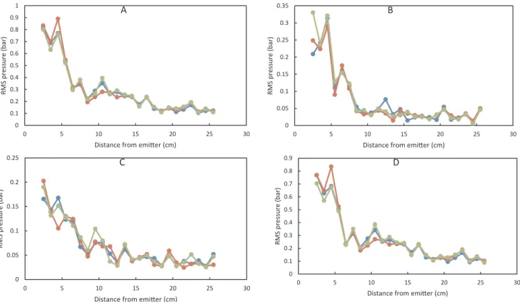
The obtained spectra are typically as illustrated inFig. 3C. They exhibit a vertical line around 20kHz corresponding to the driving (fundamental) frequency and vertical lines around multiples of 10 kHz corresponding to various (sub/ultra) harmonics. The broad-band noise lies between those lines. The amplitude/RMS pressure proﬁles obtained from the processing of the signals measured along the reactor axis are composed of 24 points, spaced of1cmand beginning2.5cmbelow the surface of the ultrasonic horn.

Repeated tests have been done without solid and withoutﬂow for an emitted power of150W. Corresponding spatial evolution curves of the RMS pressure, depicted inFig. 6, are found almost superimposed, no matter which part of the spectrum is considered. Some points located in

Fig. 4. Eﬀect of the signal duration – (A) on the fundamental peak magnitude – (B) on the broadband noise contribution to the signal power. Fig. 5. Eﬀect of the number of averaged spectra on RMS pressure of the total spectrum.

(6)

0 0.1 0.2 0.3 0.4 0.5 0.6 0.7 0.8 0.9 1 0 5 10 15 20 25 30 RMS pres su re (bar)

Distance from emiƩer (cm)

A

0 0.05 0.1 0.15 0.2 0.25 0.3 0.35 0 5 10 15 20 25 30 RMS pres su re (bar)

B

0 0.05 0.1 0.15 0.2 0.25 0 5 10 15 20 25 30 RMS pres su re (bar)

C

0 0.1 0.2 0.3 0.4 0.5 0.6 0.7 0.8 0.9 0 5 10 15 20 25 30 RMS pres su re (bar)

D

Fig. 6. Repeatability of the RMS pressure vs. axial distance from the emitter curves (emitted US power = 150 W, no solid and no liquidﬂow, 3 repetitions): (A) Total spectrum, (B) Fundamental, (C) (sub/ultra) Harmonics and (D) Broad-band noise.

Fig. 7. Fluidization of 2 mm glass beads under silent conditions with increasing and decreasingﬂow – (A) Solid hold-up – (B) Pressure drop.

0.4 0.45 0.5 0.55 0.6 0.65 0 0.01 0.02 0.03 0.04 0.05 0.06 Solid h o ld -up ( -) Fluid velocity (m/s) 0 W 60 W 90 W 160 W

Fig. 8. Fluidization of 2 mm glass beads under power ultrasound with de-creasingﬂow only – Solid hold-up.

0 0.2 0.4 0.6 0.8 1 1.2 0 5 10 15 20 25 30 Pres su re amplitude (bar)

60 W 75 W 150 W 200 W Blake threshold

Fig. 9. Eﬀect of emitted US power on the axial evolution of the pressure am-plitude at the fundamental frequency (case of non-ﬂowing liquid) and com-parison with the value of the Blake threshold calculated for 5μm diameter bubbles.

(7)

theﬁrst cm5 exhibit however a stronger variation. This zone coincides with the observed bubble cloud, which could explain the increased deviation of the measurements. Overall, the measurements show 20% deviation, which is small enough to derive reliable trends.

A strong spatial attenuation of all the signals (fundamental, har-monics, and broad-band noise) is observed over theﬁrst10cm, leading to a total RMS pressure reduced by about a factor 5. In this condition of high ultrasonic power, most of the signal consists into broad-band noise.

4. Results

4.1. Behavior of theﬂuidized bed under ultrasound

The behavior offluidization under ultrasound is first investigated. The characterization of thefluidized bed is based on the measurement

of the solid hold-up and the pressure drop through the bed over a range of liquid velocities. The pressure drop is measured by a diﬀerential manometer and the solid hold-up φ (Eq. (8)) is deduced from the measured bed height hbed( )m (the free surface of the expanded bed

being located visually): =

φ m

ρ S h

p

p bed bed ₍₈₎

withmpthe mass of the solid particles kg( ),their densityρ kg mp( . −3)and Sbedthe cross-sectional area of the column m( 2).

The results obtained for thefluidization of2mmglass beads in si-lent conditions are gathered inFig. 7. As a hysteresis behavior could be expected[35,36], measurements have been performed with both an increasing and a decreasingfluid velocity. All the curves exhibit two distinct zones separated by a slope break; they correspond to the two states of the bed:fixed and fluidized. Under silent conditions, the ex-pansion and contraction curves are almost superimposed: the solid hold-up of thefixed bed is only very slightly higher with a gradually decreasedflowrate, due to some rearrangement of the particles. The experimental data are also consistent with the Ergun equation for pressure drop in thefixed bed zone[37], and that of Wen and Yu for solid hold-up in the fluidized bed zone [38]. The low increase of pressure drop in the latter region, observed inFig. 7B, is actually due to the fact that the lowest insert is not at the very base of the column. Thus the mass of solid present between the two pressure measurement points increases with the bed expansion, so does the measured pressure drop. It has been accounted for in the line curve shown inFig. 7B (using Wen and Yu’s expression for solid hold-up).

Power ultrasound emission has little effect on fluidization behavior, as seen inFig. 8, corresponding to the bed contraction. It further im-proves the packing of thefixed bed (by about 10%) because of the vi-brations, but excepting at the highest US power the bed expansion underfluidization remains almost unchanged. Actually, at 160 W, the

0 0.1 0.2 0.3 0.4 0.5 0.6 0 5 10 15 20 25 30 RMS pres su re (bar)

A

_{60 W} 75 W 150 W 200 W 0 0.2 0.4 0.6 0.8 1 1.2 0 5 10 15 20 25 30 RMS pres su re (bar)

B

_{60 W} 75 W 150 W 200 W 0 0.05 0.1 0.15 0.2 0.25 0 5 10 15 20 25 30 RMS pres su re (bar)

C

60 W 75 W 150 W 200 W 0 0.2 0.4 0.6 0.8 1 1.2 0 5 10 15 20 25 30 RMS pres su re (bar)

D

60 W 75 W 150 W 200 W

Fig. 10. Effect of emitted US power on the axial evolution of the RMS pressure calculated over different spectrum parts – case of non-flowing liquid – (A) Fundamental frequency– (B) Total spectrum – (C) (sub/ultra) harmonics – (D) Broad-band noise.

0 10 20 30 40 50 60 70 80 90 100 0 5 10 15 20 25 30 Broad band nois e contribu Ɵ on (% )

60 W 75 W 150 W 200 W

Fig. 11. Eﬀect of emitted US power on the axial evolution of the broad-band noise contribution– case of non-ﬂowing liquid.

(8)

intense acoustic streaming deforms the bed surface, thus making di ﬃ-cult and inaccurate the measurement of its position, and probably leading to an overestimation of its height.

Our primary intention was to measure the pressure drop also under ultrasound, but we observed that the presence of gas bubbles stuck in the liquid line (due to cavitation) jeopardized the accuracy of the dif-ferential pressure measurement.

4.2. Parameter study on ultrasound propagation

Different parameters related to the ultrasound emission, the liquid flow conditions and the particle suspension were investigated, and their effects on the spectral power distribution and the signal attenuation are discussed below. For these measurements, the free surface of the ex-panded bed was set1.5cm below the US emitter (by adjusting the amount of beads for a given solid hold-up).

4.3. Eﬀect of the acoustic power

Measurements werefirst performed for the column filled with liquid only and withoutflow. The signal amplitude at the fundamental fre-quency vs. depth profile is shown onFig. 9for different values of the

emitted US power (accounting for the equipment yield measured by calorimetry). The observed tendency could first appear as counter-intuitive, as the profiles at low US power emissions are significantly higher than those at high power. With similar measurements, Son et al.

[39]observed that the fundamental amplitude profile is not affected by the emission power. However they worked at lower power (13–40 W) and seemed to be in a regime with very low broad-band noise. Con-sidering the Blake threshold as the limit amplitude necessary to ex-plosive growth of bubbles at low US frequency (and assuming for the calculation a uniform radius of 5 µm[40–42]), the most active cavita-tion zone lays above thefirst measurement point, so confined in the immediate vicinity of the emitter. However, since the Blake threshold is a model describing the behavior of an isolated bubble, using it to locate cavitation zones might be inaccurate. Indeed some authors like Nguyen et al.[30]measure a cavitation threshold around20kPafor a frequency of20kHz.

To explain the eﬀect of the acoustic power an exploration of the rest of the spectral information is needed. If obviously the same decreasing trend can be observed for the fundamental power (Fig. 10A showing equivalent RMS pressure), the RMS pressure associated with the total

0 0.2 0.4 0.6 0.8 1 1.2 1.4 0 5 10 15 20 25 30 RMS pres su re (bar)

A

0 cm/s 3.8 cm/s 6.1 cm/s 9.1 cm/s 0 0.1 0.2 0.3 0.4 0.5 0.6 0.7 0.8 0.9 1 0 5 10 15 20 25 30 RMS pres su re (bar)

B

0 cm/s 3.8 cm/s 6.1 cm/s 9.1 cm/s 0 0.1 0.2 0.3 0.4 0.5 0.6 0.7 0.8 0.9 0 5 10 15 20 25 30 RMS pressure (bar)

C

_{0 cm/s}

3.8 cm/s 6.1 cm/s 9.1 cm/s

Fig. 12. Eﬀect of liquid velocity on the axial evolution of the RMS pressure calculated over diﬀerent spectrum parts – case without solid, emitted US power = 150 W – (A) Total spectrum – (B) Fundamental frequency – (C) Broad-band noise.

0 10 20 30 40 50 60 70 80 90 100 0 5 10 15 20 25 30 Broad band nois e contribu Ɵ on (% )

0 cm/s 3.8 cm/s 6.1 cm/s 9.1 cm/s

Fig. 13. Eﬀect of liquid velocity on the axial evolution of the broad-band noise contribution– case without solid, emitted US power = 150 W.

Table 2

Attenuation coeﬃcients of 2 mm diameter particles in a 50% vol./vol. aqueous suspension.

Material Glass Polyamide

αth(Np m. −1)[47] 2.7110−4 3.1610−6

(9)

spectrum power (Fig. 10B) increases in accordance with the emitted power. Such behavior is in fact due to an energy transfer from the fundamental toward the broad-band noise when increasing the emitted power, as shown inFig. 10D. The contribution of the noise in theﬁrst

cm

10 indeed increases from less than 40% at 60 W to about 95% at 200 W (Fig. 11), suggesting a higher cavitation level. According to Yasui et al. [25], this comes with an increased numbers of bubbles, hindering also the propagation of the driving wave in the medium and leading to a faster decrease of the total power (acoustic shielding). On the other hand, the power of the (sub/ultra) harmonics (Fig. 10C) does not seem to be aﬀected by the emitted power.

4.4. Eﬀect of the liquid velocity

Over the explored range (_3.8_{cm s}_. −1−_9.1_{cm s}_. −1_{), the liquid}

ve-locity does not have any significant effect on the measured profiles. However, there is a clear difference between the cases with and without flow. The curves ofFig. 12B show a higher value of the RMS pressure measured at the driving frequency when the liquid is flowing. A probable explanation is that the bubbles are swept away by the upward flow, hence reducing the acoustic shielding. This explanation seems confirmed byFig. 12C, which shows less broad-band noise in this case, indicating less bubble activity. This thus lowers the contribution of the broad-band noise in thefirst10cm, from 85% in the quiescent liquid sonicated at 150 W to less than 60% when an upwardflow is applied (seeFig. 13).

4.5. Eﬀect of the particles

As the particles are much smaller than the wavelength (2mm vs cm

7.5 ), their eﬀect on the wave attenuation should be mainly due to

viscous losses, resulting from the oscillations of the particles in the surrounding medium, or to thermal dissipation loss, due to thermal gradients generated near the particle surface as the fluid undergoes non-isentropic periodic expansion-compression producing an oscilla-tory heatflow from/toward the particle[43,44]. Conversely, the effect

of wave scattering should be negligible[45]. Considering their much higher relative density, larger attenuation would be expected for the glass beads compared to the polyamide ones in accordance with the measurements of Dukhin et al. on similar materials [46]. Table 2

gathers the attenuation coeﬃcients corresponding to thermal losses (αth) and viscous losses (αvisc). They have been estimated from the

theoretical expressions available in Dukhin et al.[47]and He and Ni

[48], respectively, and result in rather low values.

On the other hand, the particles could provide supplementary nuclei for cavitation or interact with the generated bubbles (according to their more or less hydrophobic surface state), leading to more complex trends.Fig. 14shows the eﬀect of glass particles on power attenuation

(for the fundamental and broad-band noise, respectively), whileFig. 15

treats the case of polyamide beads. On theseﬁgures are recalled the proﬁles obtained without any solid at a liquid velocity of 6.1 cm/s (value required to achieve 40% of solid hold-up in the case of glass particles). It should be recalled that the surface of the expanded bed lies

cm

1.5 away from the US emitter, and thus the solid particles should directly affect US propagation only beyond this distance. A strong ad-ditional wave damping is observed for the fundamental in the presence of particles, especially with glass beads. In the investigated range of solid hold-up (28–50%), its effect seems however lower for glass beads than plastic ones. This might be explained by the nonlinear dependence of the wave attenuation with respect to the solid hold-up above 10% vol., as observed by previous authors in the case of particles with high density contrast[46]. The effect on the broad-band noise (Figs. 14B and

0 0.1 0.2 0.3 0.4 0.5 0.6 0.7 0 5 10 15 20 25 30 RMS pres su re (bar)

A

₀ 0.28 0.39 0.5 0 0.1 0.2 0.3 0.4 0.5 0.6 0.7 0.8 0.9 0 5 10 15 20 25 30 RMS pres su re (bar)

B

0

0.28 0.39 0.5

Fig. 14. Eﬀect of the solid hold-up on the axial evolution of the RMS pressure calculated over diﬀerent spectrum parts – case of glass particle suspension (2 mm diameter), emitted US power = 150 W– (A) Fundamental frequency – (B) Broad-band noise.

0 0.1 0.2 0.3 0.4 0.5 0.6 0.7 0 5 10 15 20 25 30 RMS pres su re (bar)

A

0 0.28 0.39 0.5 0 0.1 0.2 0.3 0.4 0.5 0.6 0.7 0.8 0.9 0 5 10 15 20 25 30 RMS pres su re (bar)

B

0

0.28 0.39 0.5

Fig. 15. Eﬀect of the solid hold-up on the axial evolution of the RMS pressure calculated over diﬀerent spectrum parts – case of plastic particle suspension (2 mm diameter), emitted US power = 150 W– (A) Fundamental frequency – (B) Broad-band noise.

(10)

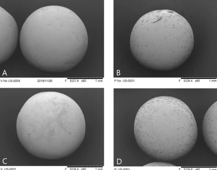
15B) is rather different whether glass or plastic particles are considered. In the case of the glass particles, the corresponding profile is almost unchanged with or without solid, while the fundamental amplitude is fast below the abovementioned 20 kPa. This could indicate a lower cavitation threshold due to the nucleation sites brought by the particles, as concluded by Tuziuti et al.[49]. In the case of plastic particles, the noise is however significantly lower, despite their higher hydro-phobicity and rugosity (see MEB pictures inFig. 16) would be expected to enhance heterogeneous nucleation of bubbles. On the other hand, Crum and Brosey [50]observed that the cavitation threshold was in-creased by small amounts of polymer additive and explained this effect by a reduced surface tension using a Harvey-type model of cavitation nucleation. As seen onFig. 16plastic particles seem slightly eroded by US, suggesting that partial dissolution of polyamide might have oc-curred under US leading to a similar mechanism. The results with solid particles would require further exploration to be fully elucidated, and in particular to decorrelate their direct influence on wave attenuation from their indirect one via cavitation threshold (due to surface defects or partial dissolution). The fact remains that acoustic cavitation is in itself an open problem and that the diversity of possible interactions between particles and bubbles precludes a purely additive effect on attenuation.

5. Conclusions

A methodology has been developed for the acoustical character-ization of sonoreactors, based on FFT signal processing, allowing to distinguish the different spectral components: driving frequency, (sub-/ ultra-)harmonics corresponding to the stable cavitation and broad-band noise associated to the inertial one. The effect of increasing emitting power on the ultrasound propagation has been studied and the results indicate a higher energy transfer from the fundamental wave toward the broad-band noise, as well as a shielding effect by the cavitation bubbles leading to a fast decrease of the total signal power with the distance from the emitter. Hence it shows that the emission power in any sonochemistry process has to be carefully chosen as higher power does not necessarily imply higher efficiency. A probable explanation of the liquidflow effect is the sweeping of the cavitation bubbles away from the zone in front of the horn. Technical restrictions indeed implied to design this reactor with ultrasound emitted against theflow, but it could be interesting to work in other configurations to check if this trend would be then modified. The solid suspension brings additional attenuation, but it is much more difficult to conclude about the causes of the observed effects. In the light of the obtained results, this study could benefit from the use of an emitting device able to generate ul-trasound at an intensity low enough to keep the medium below cavi-tation level (so as to uncouple for instance the respective effects of the

Fig. 16. MEB pictures of 2 mm glass and plastic particles before and after exposure to ultrasound– (A) Glass before US – (B) Plastic before US – (C) Glass after US – (D) Plastic after US.

(11)

[1] T.J. Mason, J.P. Lorimer, Applied Sonochemistry– The Uses of Power Ultrasound in Chemistry and Processing, Wiley-VCH, Weinheim, Germany, 2002.

[2] K.S. Suslick, Sonochemistry, Science 247 (1990) 1439–1445,https://doi.org/10. 1126/science.247.4949.1439.

[3] S. Findik, G. Gündüz, E. Gündüz, Direct sonication of acetic acid in aqueous solu-tions, Ultrason. Sonochem. 13 (2006) 203–207,https://doi.org/10.1016/j. ultsonch.2005.11.005.

[4] M.M. van Iersel, N.E. Benes, J.T.F. Keurentjes, Importance of acoustic shielding in sonochemistry, Ultrason. Sonochem. 15 (2008) 294–300,https://doi.org/10.1016/ j.ultsonch.2007.09.015.

[5] M. Sivakumar, A. Gedanken, Insights into the sonochemical decomposition of Fe (CO)5: theoretical and experimental understanding of the role of molar con-centration and power density on the reaction yield, Ultrason. Sonochem. 11 (2004) 373–378,https://doi.org/10.1016/j.ultsonch.2003.08.002.

[6] V.S. Sutkar, P.R. Gogate, Design aspects of sonochemical reactors: Techniques for understanding cavitational activity distribution and eﬀect of operating parameters, Chem. Eng. J. 155 (2009) 26–36,https://doi.org/10.1016/j.cej.2009.07.021. [7] R.A. Al-Juboori, T. Yusaf, L. Bowtell, V. Aravinthan, Energy characterisation of

ultrasonic systems for industrial processes, Ultrasonics 57 (2015) 18–30,https:// doi.org/10.1016/j.ultras.2014.10.003.

[8] M. Hodnett, 8 - Measurement techniques in power ultrasonics, Power Ultrasonics, Woodhead Publishing, Oxford, 2015, pp. 195–218 (accessed April 19, 2016). [9] R.F. Contamine, A.M. Wilhelm, J. Berlan, H. Delmas, Power measurement in

so-nochemistry, Ultrason. Sonochem. 2 (1995) S43–S47,https://doi.org/10.1016/ 1350-4177(94)00010-P.

[10] T.J. Mason, J.P. Lorimer, D.M. Bates, Quantifying sonochemistry: casting some light on a‘black art’, Ultrasonics 30 (1992) 40–42,https://doi.org/10.1016/0041-624X (92)90030-P.

[11] S. Koda, T. Kimura, T. Kondo, H. Mitome, A standard method to calibrate sono-chemical eﬃciency of an individual reaction system, Ultrason. Sonochem. 10 (2003) 149–156,https://doi.org/10.1016/S1350-4177(03)00084-1.

[12] A. Mandroyan, R. Viennet, Y. Bailly, M.-L. Doche, J.-Y. Hihn, Modiﬁcation of the ultrasound induced activity by the presence of an electrode in a sonoreactor working at two low frequencies (20 and 40kHz). Part I: active zone visualization by laser tomography, Ultrason. Sonochem. 16 (2009) 88–96,https://doi.org/10.1016/ j.ultsonch.2008.05.003.

[13] G. Mark, A. Tauber, R. Laupert, H.-P. Schuchmann, D. Schulz, A. Mues, C. von Sonntag, OH-radical formation by ultrasound in aqueous solution– Part II: ter-ephthalate and Fricke dosimetry and the inﬂuence of various conditions on the sonolytic yield, Ultrason. Sonochem. 5 (1998) 41–52,https://doi.org/10.1016/ S1350-4177(98)00012-1.

[14] B. Zeqiri, M. Hodnett, A.J. Carroll, Studies of a novel sensor for assessing the spatial distribution of cavitation activity within ultrasonic cleaning vessels, Ultrasonics 44 (2006) 73–82,https://doi.org/10.1016/j.ultras.2005.08.004.

[15] A.E. Crawford, The measurement of cavitation, Ultrasonics 2 (1964) 120–123,

https://doi.org/10.1016/0041-624X(64)90224-0.

[16] K. Yasui, T. Tuziuti, M. Sivakumar, Y. Iida, Sonoluminescence, Appl. Spectrosc. Rev. 39 (2004) 399–436,https://doi.org/10.1081/ASR-200030202.

[17] C.J.B. Vian, P.R. Birkin, T.G. Leighton, Cluster collapse in a cylindrical cell: cor-relating multibubble sonoluminescence, acoustic pressure, and erosion, J. Phys. Chem. C 114 (2010) 16416–16425,https://doi.org/10.1021/jp1027977. [18] M. Ashokkumar, The characterization of acoustic cavitation bubbles– an overview,

Ultrason. Sonochem. 18 (2011) 864–872,https://doi.org/10.1016/j.ultsonch.2010. 11.016.

[19] D. Fernandez Rivas, M. Ashokkumar, T. Leong, K. Yasui, T. Tuziuti, S. Kentish, D. Lohse, H.J.G.E. Gardeniers, Sonoluminescence and sonochemiluminescence from a microreactor, Ultrason. Sonochem. 19 (2012) 1252–1259,https://doi.org/10. 1016/j.ultsonch.2012.04.008.

[20] E. Cramer, W. Lauterborn, Acoustic cavitation noise spectra, Appl. Sci. Res. 38 (1982) 209–214,https://doi.org/10.1007/BF00385950.

[21] C. Campos-Pozuelo, C. Granger, C. Vanhille, A. Moussatov, B. Dubus, Experimental and theoretical investigation of the mean acoustic pressure in the cavitationﬁeld, Ultrason. Sonochem. 12 (2005) 79–84,https://doi.org/10.1016/j.ultsonch.2004. 06.009.

[22] V.S. Moholkar, S.P. Sable, A.B. Pandit, Mapping the cavitation intensity in an ul-trasonic bath using the acoustic emission, AIChE J. 46 (2000) 684–694,https://doi.

org/10.1002/aic.690460404.

[23] J. Frohly, S. Labouret, C. Bruneel, I. Looten-Baquet, R. Torguet, Ultrasonic cavita-tion monitoring by acoustic noise power measurement, J. Acoust. Soc. Am. 108 (2000) 2012–2020,https://doi.org/10.1121/1.1312360.

[24] Z. Liang, G. Zhou, S. Lin, Y. Zhang, H. Yang, Study of low-frequency ultrasonic cavitationﬁelds based on spectral analysis technique, Ultrasonics 44 (2006) 115–120,https://doi.org/10.1016/j.ultras.2005.09.001.

[25] K. Yasui, T. Tuziuti, J. Lee, T. Kozuka, A. Towata, Y. Iida, Numerical simulations of acoustic cavitation noise with the temporalﬂuctuation in the number of bubbles, Ultrason. Sonochem. 17 (2010) 460–472,https://doi.org/10.1016/j.ultsonch.2009. 08.014.

[26] M. Hodnett, R. Chow, B. Zeqiri, High-frequency acoustic emissions generated by a 20 kHz sonochemical horn processor detected using a novel broadband acoustic sensor: a preliminary study, Ultrason. Sonochem. 11 (2004) 441–454,https://doi. org/10.1016/j.ultsonch.2003.09.002.

[27] M. Hodnett, B. Zeqiri, Toward a reference ultrasonic cavitation vessel: Part 2-in-vestigating the spatial variation and acoustic pressure threshold of inertial cavita-tion in a 25 kHz ultrasoundﬁeld, IEEE Trans. Ultrason. Ferroelectr. Freq. Control 55 (2008) 1809–1822,https://doi.org/10.1109/TUFFC.2008.864.

[28] T. Uchida, H. Sato, S. Takeuchi, T. Kikuchi, Investigation of output signal from cavitation sensor by dissolved oxygen level and sonochemical luminescence, Jpn. J. Appl. Phys. 49 (2010) 07HE03,https://doi.org/10.1143/JJAP.49.07HE03. [29] T. Uchida, S. Takeuchi, T. Kikuchi, Measurement of amount of generated acoustic

cavitation: investigation of spatial distribution of acoustic cavitation generation using broadband integrated voltage, Jpn. J. Appl. Phys. 50 (2011) 07HE01,https:// doi.org/10.1143/JJAP.50.07HE01.

[30] T. Thanh Nguyen, Y. Asakura, S. Koda, K. Yasuda, Dependence of cavitation, che-mical eﬀect, and mechanical eﬀect thresholds on ultrasonic frequency, Ultrason. Sonochem. 39 (2017) 301–306,https://doi.org/10.1016/j.ultsonch.2017.04.037. [31] J.R. Allegra, S.A. Hawley, Attenuation of sound in suspensions and emulsions:

theory and experiments, J. Acoust. Soc. Am. 51 (1972) 1545–1564,https://doi.org/ 10.1121/1.1912999.

[32] C.M. Atkinson, H.K. Kytömaa, Acoustic wave speed and attenuation in suspensions, Int. J. Multiphase Flow 18 (1992) 577–592, https://doi.org/10.1016/0301-9322(92)90053-J.

[33] L. Gaete-Garretón, Y. Vargas-Hernández, S. Pino-Dubreuil, F. Montoya-Vitini, Ultrasonic detectors for high-intensity acousticﬁelds, Sens. Actuators, A 37–38 (1993) 410–414,https://doi.org/10.1016/0924-4247(93)80070-W. [34] M. Cerna, A.F. Harvey, The Fundamentals of FFT-based Signal Analysis and

Measurement, National Instruments Application Note 041, 2000.

[35] J.P. Riba, R. Routie, J.P. Couderc, Conditions minimales de mise enﬂuidisation par un liquide, Can. J. Chem. Eng. 56 (1978) 26–30,https://doi.org/10.1002/cjce. 5450560104.

[36] R. Di Felice, Hydrodynamics of liquidﬂuidisation, Chem. Eng. Sci. 50 (1995) 1213–1245,https://doi.org/10.1016/0009-2509(95)98838-6.

[37] S. Ergun, Fluidﬂow through packed columns, Chem. Eng. Prog. 48 (1952) 89–94. [38] C.Y. Wen, Y.H. Yu, Mechanics of Fluidization, Chem. Eng. Prog. Symp. Ser. 62

(1966) 100–111.

[39] Y. Son, M. Lim, J. Khim, M. Ashokkumar, Acoustic emission spectra and sono-chemical activity in a 36kHz sonoreactor, Ultrason. Sonochem. 19 (2012) 16–21,

https://doi.org/10.1016/j.ultsonch.2011.06.001.

[40] F. Burdin, N.A. Tsochatzidis, P. Guiraud, A.M. Wilhelm, H. Delmas,

Characterisation of the acoustic cavitation cloud by two laser techniques, Ultrason. Sonochem. 6 (1999) 43–51,https://doi.org/10.1016/S1350-4177(98)00035-2. [41] R. Mettin, S. Luther, W. Lauterborn, Bubble size distribution and structures in

acoustic cavitation, in: Proceedings of 2nd Conference on Applications of Power Ultrasound in Physical and Chemical Processing, Toulouse, France, 1999, pp. 125–129.

[42] O. Louisnard, A simple model of ultrasound propagation in a cavitating liquid. Part I: theory, nonlinear attenuation and traveling wave generation, Ultrason. Sonochem. 19 (2012) 56–65,https://doi.org/10.1016/j.ultsonch.2011.06.007. [43] P.S. Epstein, R.R. Carhart, The absorption of sound in suspensions and emulsions. I.

Water fog in air, J. Acoust. Soc. Am. 25 (1953) 553–565,https://doi.org/10.1121/ 1.1907107.

[44] P.M. Morse, K.U. Ingard, Theoretical Acoustics, Princeton University Press, 1986. [45] M. Su, M. Xue, X. Cai, Z. Shang, F. Xu, Particle size characterization by ultrasonic

attenuation spectra, Particuology 6 (2008) 276–281,https://doi.org/10.1016/j. partic.2008.02.001.

[46] A.S. Dukhin, P.J. Goetz, Acoustic spectroscopy for concentrated polydisperse col-loids with high density contrast, Langmuir 12 (1996) 4987–4997,https://doi.org/ 10.1021/la951085y.

[47] A.S. Dukhin, P.J. Goetz, C.W. Hamlet, Acoustic spectroscopy for concentrated polydisperse colloids with low density contrast, Langmuir 12 (1996) 4998–5003,

https://doi.org/10.1021/la951572d.

[48] G. He, W. Ni, Ultrasonic attenuation model for measuring particle size and inverse calculation of particle size distribution in mineral slurries, J Cent. South Univ. Technol. 13 (2006) 445–450,https://doi.org/10.1007/s11771-006-0065-x. [49] T. Tuziuti, K. Yasui, M. Sivakumar, Y. Iida, N. Miyoshi, Correlation between

acoustic cavitation noise and yield enhancement of sonochemical reaction by par-ticle addition, J. Phys. Chem. A 109 (2005) 4869–4872,https://doi.org/10.1021/ jp0503516.

[50] L.A. Crum, J.E. Brosey, Eﬀect of dilute polymer additives on the acoustic cavitation threshold of water, J. Fluids Eng. 106 (1984) 99–104,https://doi.org/10.1115/1. 3242413.

bubble cloud and of the solid particles on the wave attenuation). This work will be followed by an experimental investigation of the local mass transfer coeﬃcient (measured by electrochemical method) under the same conditions and in the same sonoreactor, so as to cor-relate its enhancement to the cavitation intensity and power repartition in the acoustic spectrum.

Acknowledgements

The authors thank B. Boyer and E. Prevot (LGC Toulouse) for technical support on the experimental setup and M.L. de Solan Bethmale (SAP, LGC Toulouse) for the MEB pictures of the particles. References