To link to this article : DOI:10.1016/j.rser.2013.08.042
URL :
http://dx.doi.org/10.1016/j.rser.2013.08.042
O
pen
A
rchive
T
OULOUSE
A
rchive
O
uverte (
OATAO
)
OATAO is an open access repository that collects the work of Toulouse researchers and
makes it freely available over the web where possible.
This is an author-deposited version published in :
http://oatao.univ-toulouse.fr/
Eprints ID : 9348
To cite this version : Belouda, Malek and Jaafar, Amine and Sareni,
Bruno and Roboam, Xavier and Belhadj, Jamel Integrated optimal
design and sensitivity analysis of a stand alone wind turbine system
with storage for rural electrification. (2013) Renewable and Sustainable
Energy Reviews, 28 . pp. 616-624. ISSN 1364-0321
Any correspondance concerning this service should be sent to the repository
administrator:
[email protected]
Integrated optimal design and sensitivity analysis of a stand alone
wind turbine system with storage for rural electrification
M. Belouda
a,b,n, A. Jaafar
c, B. Sareni
c, X. Roboam
c, J. Belhadj
a,baUniversity of Tunis, DGE-ESSTT, Tunisia
bUniversity of Tunis El Manar, ENIT, L.S.E.B.P. 37, 1002 Tunis, Tunisia
cUniversité de Toulouse, LAPLACE UMR CNRS-INP-UPS, ENSEEIHT 2, Rue Charles Camichel 31071, Toulouse, France
Keywords: Passive wind turbine Systemic optimization Integrated Optimal Design Battery cycles
Total cost of ownership Sensitivity analysis
In this paper, the authors investigate a robust Integrated Optimal Design (IOD) devoted to a passive wind turbine system with electrochemical storage bank: this stand alone system is dedicated to rural electrification. The aim of the IOD is to find the optimal combination and sizing among a set of system components that fulfils system requirements with the lowest system Total Cost of Ownership (TCO). The passive wind system associated with the storage bank interacts with wind speed and load cycles. A set of small power passive wind turbines spread on a convenient power range (2–16 kW) are obtained through an IOD process at the device level detailed in previous papers. The system cost model is based on data sheets for the wind turbines and related to battery cycles for the storage bank. From the range of wind turbines, a “system level” optimization problem is stated and solved using an exhaustive search. The optimization results are finally exposed and discussed through a sensitivity analysis in order to extract the most robust solution versus environmental data variations among a set of good solutions.
Contents
1. Introduction . . . 2
2. Description of the system . . . 2
3. Systemic optimization procedure . . . 3
4. Local optimization . . . 3
5. Systemic optimization . . . 3
5.1. WT cost model. . . 4
5.2. Battery bank cost model based on cycling effects . . . 4
5.3. Optimization problem formulation . . . 5
5.3.1. TCO . . . 5
5.3.2. Design variables . . . 5
5.3.3. Optimization constraints . . . 5
6. Results and sensitivity analysis . . . 6
6.1. Optimization results . . . 6
6.2. Sensitivity analysis of optimal solutions versus environmental data variations . . . 7
6.2.1. Sensitivity versus wind speed profile changes . . . 7
6.2.2. Sensitivity versus load profile changes . . . 8
7. Conclusion . . . 8 Acknowledgment . . . 8 Appendix . . . 8 References . . . 9 http://dx.doi.org/10.1016/j.rser.2013.08.042 n
Correspondence to: School of Sciences and Technology of Tunis (ESSTT), 5 Avenue Taha Hussein, (B.P. 56 Bab Menara), 1008 Montfleury-Tunis, Tunisia. Tel.: þ 216 99 61 41 14.
1. Introduction
According to the World Energy Agency [1], some 1.5 billion people had no access to electricity in the world by 2009, with more than 80% of habitants in rural zones. Providing consumers in remote areas with reliable and cheap electricity becomes a priority in several developed and undeveloped countries such as in the case of isolated cities in Tunisia. The steadily increasing demand of fossil fuels along with concerns about global warming, presents natural renewable energy sources as attractive solutions. Among these sources wind energy systems (free in their availability, renewable and non-polluting) with storage are among the most competitive alternatives for electrifying remote consumers and they are widely used in both autonomous or grid connected applications. These systems can also operate in parallel with others available energy sources (fuel cells, diesel generators) and several means of storage (accumulators, H2storage, etc.) in order
to enhance the system reliability[2–5].
However, the drawbacks of such sources are their TCO which is still expensive, especially for small wind turbine systems. More-over to assure the service continuity and to protect the battery against deep discharges (subsequently extend the battery bank life), such systems require an additional dynamic source of energy or an optimal wind system design [8,9]). Recently, several researches based on global optimization techniques have been focused on the design of optimal system configurations which meet the load demand for given climatic data[10–12].
Bagul, Borowy and Salameh [6–8] have developed several methodologies for optimally sizing a wind/PV system associated with a battery bank for a given load. These methods are based on the use of long term data for both irradiance and wind speed. However, such approaches are penalized by CPU time due to wide data range. Several studies have used the average hourly wind speed data over a few years simulation period, but this vision strongly filters wind turbine powers. Other researchers [13,14]
have developed probabilistic methods to determine the annual energy of a wind system. In particular in[15–19], authors have selected the optimal combination and sizing of wind generators, PV modules and storage batteries.
This paper suggests a systemic methodology for designing the optimal combination and sizing of passive wind turbines asso-ciated with electrochemical storage. Generally, deterministic opti-mization approaches neglect the effects of environmental inputs uncertainties (including variation or perturbation of wind speed and/or load profiles) which can lead to drastic change of optimal solution quality. Several studies[20–26]have taken into account
the increased need for sensitivity analyses to perform a robust system design in various research areas.Thus, this study is parti-cularly focused on the sensitivity analysis of a set of “good” solutions to obtain an optimum system quite insensitive to environmental variations.
The remaining of the paper is organized as follows. The passive wind system and the battery characteristics are described in
Section 2. In the third section, the systemic optimization proce-dure is presented.Section 4is dedicated to the local optimization procedure. The models and the systemic optimization formulation are exposed inSection 5.Section 6is reserved to the results and the sensitivity analysis.
2. Description of the system
The considered system is a “low cost” full passive wind turbine (WT) battery charger (Fig. 1) without active control and with minimum number of sensors as studied in [27,28]: this local optimization loop is not detailed in this paper but only referred to previous studies. An experimental prototype of the optimized system, especially the PM synchronous generator, has been built in LAPLACE Lab and had confirmed the ability of the passive structure to draw a power close to the optimal range with small losses. This prototype and subsequent study is detailed in [29]. The wind turbine parameters have been obtained by applying similitude relationships with reference to a 1.7 kW wind turbine which had been previously optimized by the local IOD process in[30,31].
Both wind speed and load profiles used in this study are considered as deterministic data. These data were acquired at a typical farm in Tunisia. The load profile is set on 24 h and day by day repeated (Fig. 2). The wind speed profile has been obtained from a previous study [32] by applying a “compact synthesis process” on an actual wind speed profile of 200 days duration considered as reference data, with the aim of generating a
C U DC IDC Load profile Wind turbine Vwind B a tt er y b a n k PMSG
Fig. 1. WT system with battery for stand alone application (rural site electrification).
Nomenclature
c scale factor (m/s)
C0 cost of one deep battery cycle (€)
C3 battery element nominal capacity (Ah)
CBAT battery bank cost (€)
CCell battery cell cost (€)
CF cycle to failure
CWT wind turbine cost (k€)
DOD depth of discharge
I3 battery element nominal discharge current (A)
Icel battery cell current (A)
Ich_max battery cell maximum charge current (A)
Idisch_max battery cell maximum discharge current (A)
k shape factor
N number of cycles at a given DOD Ncel_p number of cells in parallel
Ncel_s number of cells in series
NCH number of the battery bank changes over 20 years
Ncyc equivalent number of cycles
Nτ
cyc equivalent number of cycles
Pext extracted power (W)
Pload load power (W)
PWT wind turbine nominal power (W)
SOC battery cell state of charge Taut battery bank time autonomy (h)
TCO total cost of ownership (k€) V0 battery element nominal voltage (V)
V1,2,3 generated wind speed (m/s)
Vref reference compact wind speed (m/s)
Vwind wind speed (m/s)
wcyc weight of a cycle
τ repeated wind cycle (days) τop operating period (days)
compact profile on a reduced duration of 10 days (Fig. 3) to accelerate the optimization process. It should be noted that this process synthesizes a wind cycle which fulfils the main character-istics of the reference cycle on 200 days, especially the maximum wind speed, the average cubic wind speed and the energy content of the wind cycle[32].
In this study, a lead acid Yuasa NP 38-12I[33]is considered as battery element. The basic characteristics are summarized in
Table 1.
NB: in the following, let us note that the 12 V Yuasa “battery element” is constituted of 6 “cells” of 2 V in series. The association of several “battery elements” (12 V) in series and in parallel will be named as “battery bank”.
3. Systemic optimization procedure
In order to perform the optimization of the whole system including the passive WT and the storage battery considering wind speed and consumption profiles, we have adopted an approach based on two optimization levels:
Level 1 Systemic Optimization (SO) of the whole system. Level 2 Local Optimization (LO) of the WT device.
Given a wind speed profile, the SO approach consists in selecting a WT in the range normally provided by the WT manufacturer (WT T1–Tnand the corresponding Permanent
Mag-net Synchronous Generator (PMSG) G1–Gn: in our case, these
devices are obtained from the LO process as presented in[31]). The couple (Ti, Gi) and the corresponding storage sizing have to
satisfy a given load demand at lowest TCO. This compromise can
be obtained by solving the optimization problem illustrated in
Fig. 4.
4. Local optimization
The aim of this second optimization level is to build a range of n generators corresponding to n WTs which will be used in the first optimization level (systemic approach). In this approach, the battery bank voltage is as constant and equal to 48 V (i.e. a series connection of 4 Yuasa 12 V elementary batteries) (Fig. 5).
The “mixed reduced model” considered in this optimization process is detailed in[27,31].
In[31], an IOD method, based on a multiobjective optimization, has been developed for sizing the elements of a 1.7 kW passive wind turbine system. The WT range with related generator parameters for various nominal powers has been obtained by applying similitude relationships with reference to the 1.7 kW wind turbine system[30].Fig. 6shows the extracted powers Pextof
the passive wind turbines (till 16 kW) obtained by similitude from the optimized reference passive wind turbine of 1.7 kW
(Appendix). It can be seen that the quality of wind power extraction of these passive configurations (solid curves) matches very closely the behavior of active wind turbine systems operating at optimal wind powers by using an MPPT control device (i.e. the cubic curves inFig. 6). It should be noted that the selected wind turbine range (1.7 up to 16 kW) is constrained by the average load power 〈Pload〉, since we have adopted a range between ½ 〈Pload〉and
5 〈Pload〉. Furthermore, the use of similitude models from a
reference wind turbine device of 1.7 kW limits the range of power expansion to fulfill validity domain of similitude relationships.
0 2 4 6 8 10 0 5 10 15 20 25 Time (days) Vwind (m/s)
Fig. 3. Wind speed compact profile.
Wind cycle WT Batteries Load WT manufacturer range T1 G1 T2 G2 Tn Gn Local Optimization (LO) Systemic Optimization (SO) PMSG
Fig. 4. Systemic Optimization process.
WT and PMSG Sizing by similitude C Vwind IDC PMSG UDC=48V UDC=48V
Fig. 5. Passive WT synoptic. Table 1
Basic characteristics of a Yuasa NP 38-12I lead acid battery element.
Nominal capacity C3 30.3 (Ah)
Nominal voltage V0 12 (V)
Nominal discharge current I3 10.1 (A)
0 0 2 4 6 Time(h) PLoad/day ( kW) 24 21 18 15 12 9 6 3
5. Systemic optimization
The aim of the SO stage is the minimization of the TCO on a life cycle of 20 years of the passive WT coupled with a storage bank ensuring the electrification of the isolated farm under a specific compact wind speed cycle [32]. To achieve this optimization process, a cost model of each system component has to be determined.
5.1. WT cost model
Generally, the WT subsystem is composed of a turbine, a nacelle, a tower, a rectifier, a mechanical transmission system. There is no single component that dominates the WT cost. Typical owning costs given by “eaglewestwind”[34]for a range of turbines from 2 kW up to 20 kW are shown inFig. 7: system costs include costs due to all components of the device. A linear interpolation of these costs has led to the following WT cost model:
CWT¼ 1:7PWTþ 3 ð1Þ
The lifetime of WTs being assumed to be at least 20 year, the owning cost of WTs will simply be due to the investment cost, which assumes that no maintenance costs are needed due to the robustness of the full passive wind turbine structure. Such assumption can be justified for low power wind turbines, espe-cially as the passive structure is particularly robust.
5.2. Battery bank cost model based on cycling effects
The battery cost depends on the charge and discharge cycling in terms of number and cycle depth that the battery can provide (battery lifetime strongly depend on both depth and rate of discharge). The equivalent number of cycles (Ncyc) is obtained by
a weighted sum of the cycles in terms of their depth of discharge (DOD). The weights are derived from the manufacturer curve giving the number of complete cycles that the storage element is
0 50 100 0 0.5 1 1.5 1 0 50 100 0 1 2 3 2 0 20 40 60 80 0 1 2 3 4 3 0 20 40 60 70 0 2 4 6 4 0 50 0 2 4 6 5
P
ext(kW)
00 20 40 60 2 4 6 8 6 0 20 40 60 0 5 10 7 0 20 40 60 0 5 10 8 0 50 0 5 10 9 0 20 40 50 0 5 10 15 10 0 20 40 50 0 5 10 15 11 0 20 40 0 5 10 15 12 0 20 40 0 5 10 15 13 0 20 40 0 10 20 14 0 20 40 0 10 20 15 0 20 40 0 5 10 15 20 16Ω (rd/s)
Fig. 6. Extracted power of the range of passive WT systems obtained by similitude from the reference 1.7 kW WT.
0 5 10 15 20 0 5 10 15 20 25 30 35 40 PWT kW) CW T ( k € ) CWT = 1.7 PWT + 3
capable of delivering in terms of its DOD (characteristic called “cycle to failure”).
The lifetime model, for Yuasa NP 38-12I lead acid battery, uses an exponential curve fitting based on the available cycle to failure (CF) curve (Fig. 8) versus DOD[35,36,37]:
CF¼ 177:77 þ 7807:39:e
#6:75:DOD
ð2Þ Considering the number of cycles provided by the battery with a DOD of 100% as a reference, the weight of a cycle depth DOD (wcyc(DOD)) is expressed by the following equation:
wcycðDODÞ ¼
CFð100%Þ
CFðDODÞ ð3Þ
Thus, the equivalent number of cycles is obtained by: Ncyc¼∑
DOD
wcycðDODÞ $ NðDODÞ ð4Þ
where N(DOD) is the number of cycles at a given DOD obtained by the Rainflow method.
For an operating period τop of 20 years and a repeated wind
cycle τ of 10 days, the approximate cost of the battery bank, taking account of cycling constraints over 20 years, is expressed by the following equation:
CBATðk€Þ ¼ Ncel_sNcel_pC0$ 10#3Nτcyc
τop τ
ð5Þ where Ncel_s is the number of battery cells of 2 V associated in
series (here considered as constant and equal to 24 to constitute a battery of 48 V), Ncel_pis the number of battery cells associated in
parallel and C0is the cost of one deep battery cycle (DOD¼100%)
estimated at 0.1 €[33]. This latter cost comes from the Yuasa 12 V battery element cost which is 108 €. Then, the 2 V battery cell cost is CCell¼ 108/6 € for 180 allocated deep cycles. Finally, one cell deep
cycle cost is CCell/180 ¼0.1 €.
It should also be noted that the initial purchase cost of the battery CBAT0is defined as following:
CBAT0ðk€Þ ¼ Ncel_sNcel_pCCell$ 10#3 ð6Þ
5.3. Optimization problem formulation
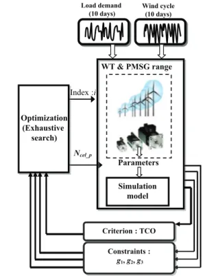
The problem is to develop a systemic approach that allows optimizing system configurations (passive WT with storage bank) that satisfy load power demand with minimum TCO. The TCO calculation includes the WT owning cost and battery bank owning cost. The systemic optimization process is detailed in Fig. 9. By means of the compacted wind cycle obtained from the synthesis process proposed in[32](as presented inFig. 3), only 10 days of system operation have to be simulated in this optimization process. Results obtained from this typical but representative
compact profile are then extrapolated over 20 years in order to estimate the TCO due to cycling effects.
5.3.1. TCO
A single objective function is used consisting in the TCO which includes WT and battery bank owning costs over a duration period of 20 years.
TCO ¼ CWTþ CBAT ð7Þ
5.3.2. Design variables
The optimization problem only uses two discrete design variables:
%
Ncel_p: The number of battery cells associated in parallel (Ncel-s_being the number of battery cells (2 V) in series is fixed at 24 for a 48 V battery bank).
%
index i: This index identifies the couples of turbines and associated generators (Tiand Gi) used in the simulation model for computingthe system TCO and the optimization constraints. Note also that this index corresponds with power level (in kW) of the WT. 5.3.3. Optimization constraints
%
g1: is a constraint related to the maximum discharge current(Idisch_max).
The battery cell maximum discharge current (max(Icel)), must
be less than the current Idisch_max:
g1¼ max IðcelÞ#Idisch_ maxr0 ð8Þ
%
g2: is a constraint related to maximum charge current (Ich_max).The absolute value of the maximum battery cell charge current (│min(Icel)│) must be less than the current Ich_max:
g2¼ min IðcelÞ#Ich_ maxr0 ð9Þ Note that charge/discharge current are respectively considered as negative/positive. 0.1 0.2 0.3 0.4 0.5 0.6 0.7 0.8 0.9 1 100 1000 180 3000 5000 500
Depth of discharge DOD
C y c le t o f a il u re C F
Fig. 8. Cycle to failure curve for Yuasa accumulator cell.
Index :i I Optimization (Exhaustive search) Parameters Wind cycle (10 days) Ncel_p Load demand (10 days) Simulation model WT & PMSG range Constraints : g1, g2, g3 Criterion : TCO
%
g3: is a constraint related to the battery cell state of charge(SOC).
The minimum value of the battery cell state of charge min(SOC (t)) must be greater than 20%:
g3¼ 20%# min SOC tð ð ÞÞ r 0 ð10Þ In this study, Idisch_maxand Ich_maxhave been chosen equal to the
nominal discharge current I3¼ 10.1 A (Table 1).
As defined, the optimization problem is sufficiently simplified (one objective, two design variables and three constraints) to justify the use of an exhaustive search (80.14¼ 1120 combinations) instead of adopting more sophisticated optimization algorithms. Other approaches may be used in more complex case study, as for hybrid systems with several sources. Note also that this simplified and efficient optimization problem is mainly due to the structure of the design process with 2 loops, one for the WT device and another one for systemic approach.
6. Results and sensitivity analysis 6.1. Optimization results
Fig. 10 shows a set of solutions resulting from the systemic optimization process, corresponding to a TCO lower than 115.5 k€. It should be observed that the TCO range is displayed with a reduced scale (1/115 k€) so that TCOs of these solutions can be considered as quasi-equivalent. Each point corresponds to one solution, (i.e. one couple of variables: index i representing the WT rated power and Ncel-p). The cheapest solution (circled inFig. 10)
corresponds to a configuration with 63 branches in parallel (i.e. 252 “12 V Yuasa battery elements” for the battery bank) with a WT of 13 kW of nominal power (i¼13).Table 2 gives the different characteristics of some quasi-equivalent optimal solutions and
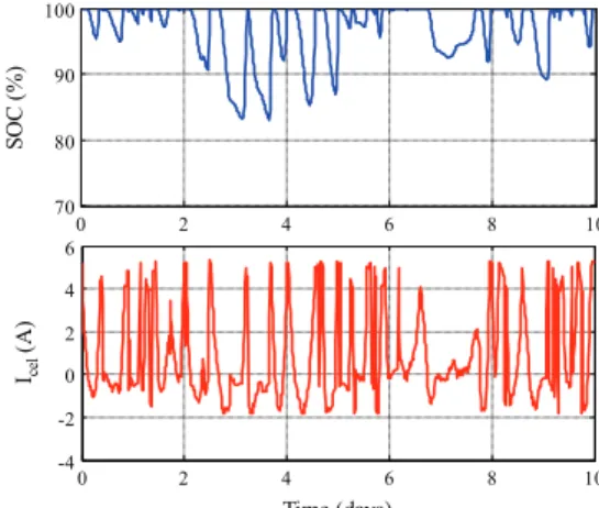
Fig. 11shows the state of charge SOC and the battery cell current (Icel) evolutions of the solution Sol 13opt. One can see that a
reduced DOD range is obtained from that optimal sizing taking account of cycling effect on system costs.
Note that NCH is the number of the battery bank changes
necessary for 20 years. NCHcan be calculated from(5)and(6)by
deriving the following equation: NCH¼
CBATover 20 years
CBAT0
ð11Þ
Another criterion necessary for the optimal solutions analysis is the battery bank autonomy time Tautof each solution. This time is
defined as the corresponding duration of a complete battery discharge up to 20% of SOC, considering the load profile without any wind power production.Table 3displays the autonomy time of each solution.
Fig. 12confirms the example ofFig. 11by illustrating a major trend: optimization of TCO strongly limits variations of battery SOC (reduced values of DOD) in order to enhance its lifetime. Results would have been completely different if the cycling was not taken into account through the system TCO. In such a case, the whole range of DOD would be exploited with deep discharge cycles.
The analysis of the results summarized in Table 2illustrates that some optimized solutions with different characteristics have almost the same TCO. The solutions indexed 15(a), 15(b) (PWT¼ 15 kW) and 16(a), 16(b) (PWT¼ 16 kW) correspond with the
cheapest battery owning cost CBAT among others configurations.
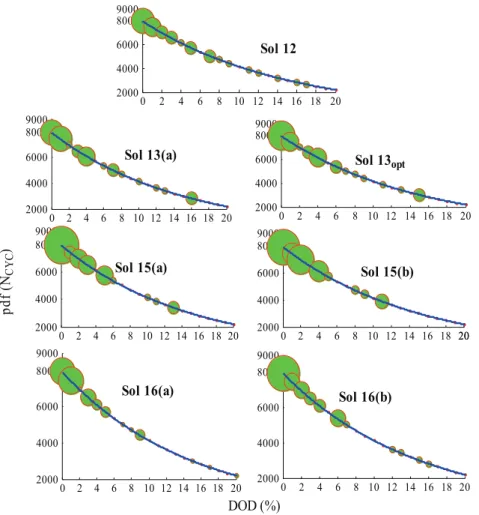
The choice of the solution indexed 13 is optimal in terms of TCO, but nearly equivalent and surely not the most relevant solution regarding other criteria as the system autonomy.Fig. 12shows the curves of the probability density functions (pdf) of the number of cycles versus the depth of discharge (DOD) and their locations on the corresponding “cycle to failure” curve for each solution. The circle diameter on the “cycles to failure” curve is proportional to the cycle occurrence, i.e. the equivalent pdf. These figures show that the maximum of DOD for all solutions does not exceed 23% of the total storage capacity of the battery bank. These results explain why there is a trend to increase the number of battery cells in the solution Sol 15(a) compared with the solution Sol 16(a): this is obviously to further expand the total storage capacity of the battery bank and to reduce subsequently deep discharge cycles therefore enhancing the lifetime.
45 50 55 60 65 70 75 80 114 114.2 114.4 114.6 114.8 115 Ncel-p TCO (k€) Sol 15(a) Sol 16(a) Sol 13opt Sol 16(b) Sol 12 Sol 13(a) Sol 15(b)
Fig. 10. Similar solutions with equivalent TCO.
0 2 4 6 8 10 70 80 90 100 S O C ( % ) 0 2 4 6 8 10 -4 -2 0 2 4 6 Time (days) Icel (A )
Fig. 11. SOC and Icelevolutions for the optimal solution.
Table 3
Time autonomy of quasi-equivalent optimal solutions.
Sol 16(a) Sol 16(b) Sol 12 Sol 13(a) Sol 13opt Sol 15(a) Sol 15(b)
Taut(h) 5 6 6.2 6.4 6.6 7.1 8.1
Table 2
Quasi-equivalent optimal solutions characteristics.
Sol 16(a) Sol 16(b) Sol 12 Sol 13(a) Sol 13opt Sol 15(a) Sol 15(b) Ncel_p 49 59 61 62 63 69 79 CWT(k€) 30 30 23 25 25 28.5 28.5
NCYC(on 20 years) 714 594 622 602 589 520 452
CBAT(k€) 84.1 84.2 91 89.7 89.1 86.2 85.8
TCO (k€) 114.3 114.4 114.5 114.8 114.2 114.7 114.3 CBAT0(k€) 21 25.4 26.3 26.7 27.2 29 34.1
Furthermore, at equivalent system cost, it is certainly prefer-able to dispose of a greater storage capacity in order to ensure load demands during longer periods without wind (i.e. autonomy
Table 3). More generally, it is interesting to analyze these solutions by sensitivity analysis versus changes of environmental data (wind speed and load) then to rebuild the optimization problem to choose a robust and optimal solution.
6.2. Sensitivity analysis of optimal solutions versus environmental data variations
This section is devoted to the sensitivity analysis of the equivalent optimal solutions presented inFig. 10versus environ-mental input changes (i.e. wind speed and load profile variations) with the aim of identifying the most robust solutions.
6.2.1. Sensitivity versus wind speed profile changes
Equivalent optimal solutions represented inFig. 10have been obtained for a particular wind speed compact profile (Vref) (see
Fig. 3). Vref distribution corresponds to the characteristics of a
Weibull law with a scale factor c¼ 9.5 m/s and a shape factor k¼ 2.3. Here, we aim at analyzing solution robustness versus statistic characteristics mentioned inTable 4.
For this purpose, three particular time profiles of wind speed with 200 days duration are generated from different Weibull distributions (V1, V2, V3) as displayed inFig. 13and characterized inTable 4.
Table 5 gives the number of cycles over 20 years NCYC, the
battery bank cost CBATand the TCO of several equivalent optimal
solutions for each wind speed profile. These results show that the solution Sol 15(b) is the most robust in terms of TCO change: (Sol 15(b) remains lower than the one obtained with other solutions whatever the wind conditions. This robustness is partly due to the
0 2 4 6 8 10 12 14 16 18 20 2000 4000 6000 8000 9000
p
d
f
(N
C Y C)
0 2 4 6 8 10 12 14 16 18 20 2000 4000 6000 8000 9000 0 2 4 6 8 10 12 14 16 18 20 2000 4000 6000 8000 9000 0 2 4 6 8 10 12 14 16 18 20 2000 4000 6000 8000 9000 0 2 4 6 8 10 12 14 16 18 20 2000 4000 6000 8000 9000 0 2 4 6 8 10 12 14 16 18 20 2000 4000 6000 8000 9000 0 2 4 6 8 10 12 14 16 18 2020 2000 4000 6000 8000 9000DOD (%)
Sol 12
Sol 13(a)
Sol 13
opt
Sol 15(a)
Sol 16(b)
Sol 15(b)
Sol 16(a)
Fig. 12. pdf of NCYCversus DOD on cycle to failure curve of each solution.
Table 4
Wind speed profiles characteristics.
c k Vmin Vmax 〈V〉 〈V3〉 Vref 9.5 2.3 0.1 25 8.3 1195 V1 9 2 0.04 25.3 8 867 V2 10 2 0.04 31.6 8.9 1189 V3 12 2 0.1 34.5 10.8 2072 0 5 10 15 20 25 0 0.02 0.04 0.06 0.08 0.1 V(m/s) p d f( V ) V3 : c=12 k=2 V1 : c=9 k=2 V2 : c=10 k=2
battery capacity of the Sol 15 (b) (Ncel_p¼ 79) which is the highest
among all other solutions.
6.2.2. Sensitivity versus load profile changes
The sensitivity analysis of the optimal solutions versus load profile is performed by considering an actual wind profile of one year duration (V) whose characteristics are given in Table 6. Changes made with respect to the original load profile consist in inserting a variation of 25% of load power during the even days and #25% during odd days (Fig. 14).
Table 7 shows that the Sol 15(b) remains the most robust solution in terms of TCO versus variations of load profile. As mentioned in the case of wind speed profile variations, this is explained by the highest storage capacity.
Beyond this sensitivity analysis, we can guess that the solution with the highest battery capacity (Sol 15 (b)) is also the most autonomous in case of wind drops: it is subsequently the most reliable and relevant for this application.
7. Conclusion
This paper illustrates a systemic optimization approach devoted to the optimal design of a full passive WT with storage
dedicated to stand alone applications (here for rural electrification purpose). System environment, especially wind and load condi-tions is integrated in the systemic design by optimization. The integrated optimal design problem was divided into two optimiza-tion processes: a local optimizaoptimiza-tion which aims at designing a set of optimized WT in order to constitute a manufacturer range to be used in the second optimization process dedicated to the whole system design. The systemic optimization objective is to minimize the total owning system cost, integrating simultaneously WT and battery costs by taking account of the number of device change due to cycling effects. It is interesting to note that such a systemic vision of the TCO over the whole life cycle (here 20 years) leads to oversize batteries in order to reduce DODs (lower than 20%) in order to reduce the number of device changes over the 20 years. Optimal results were analyzed and discussed then completed by a sensitivity analysis which has compared several selected solutions previously considered as quasi-equivalent. The sensitivity of these quasi-optimal solutions has been analyzed versus changes of environmental data (wind speed and load profiles variations) showing that solutions with highest storage capacity were the most relevant, being the most robust and also the most autono-mous in case of lack of wind. The availability of the developed methodology was successfully demonstrated with the considered environmental data and it is appropriated for other acquired sets of experiment data to find consistently the optimal generation system design.
Acknowledgment
This work was supported by the Tunisian Ministry of High Education, Research and Technology; CMCU 12G1103 and INPT SMI Projects. 0 1 2 0 2 4 6 8 Days PL o ad (k W ) Odd day
Original load profile
Changed load profile
Even day
Fig. 14. Load profile changes.
Table 7
Sensitivity versus load profile variations. Sol 16 (a) Sol 16 (b) Sol 12 Sol 13 (a) Sol 13opt Sol 15 (a) Sol 15(b) Original profile Ncyc 824 655 842 761 746 578 495 CBAT (k€) 97 92 123 113 112 95 94 TCO (k€) 127 122 146 138,4 138 124 122 Modified profile Ncyc 791 650 811 746 728 573 479 CBAT (k€) 93 92 118 111 110 94 90 TCO (k€) 123 122 142 136 135 123 119 Table 5
Wind speed profile variations results.
Sol 16(a) Sol 16(b) Sol 12 Sol 13(a) Sol 13opt Sol 15(a) Sol 15(b)
Vref Ncyc 714 594 622 602.98 589 520 452 CBAT(k€) 84.1 84.2 91.1 89.7 89 86.2 85.8 TCO (k€) 114.32 114.40 114.38 114.86 114.25 114.74 114.37 V1 Ncyc 1015 829 995 924 900 728 623 CBAT(k€) 119 117 145 137 136 120 118 TCO (k€) 149 147 169 162 161 149 146 V2 Ncyc 846 659 806 752 736 582 480 CBAT(k€) 99 93 118 111 111 96 91 TCO (k€) 129 123 141 137 136 124 119 V3 Ncyc 653 455 557 499 492 402 340 CBAT(k€) 76 64 81 74 74 66 64 TCO (k€) 107 94 104 99 99 95 92 Table 6
Wind speed profile V characteristics.
c k Vmin Vmax 〈V〉 〈V3〉
Appendix
SeeTables A1andA2. References
[1]International Energy Agency, World Energy Outlook; 2009.
[2]Weisser D. On the economics of the electricity consumption in small island developing states: a role for renewable energy technologies? Energy Policy 2004;32(1):127–40.
[3]Nakata T, Kubo K, Lamont A. Design for renewable energy systems with application to rural areas in Japan. Energy Policy 2005;33(2):209–19. [4]Castle JA, Kallis JM, Marshall NA, Moite SM. Analysis of merit of hybrid wind/
photovoltaic concept for stand alone systems. In: Proceedings of 15th IEEE PV specialists; 1981.
[5]Nayer CV, Phillip SJ, James WL. Novel wind/diesel/battery hybrid energy system. Solar Energy 1993;51(1):65–8.
[6]Borowy BS, Salameh ZM. Optimum photovoltaic array size for a hybrid wind/ PV system. IEEE Transactions on Energy Conversion 1994;9(3):482–8. [7]Bagul AD, Salameh ZM, Borowy BS. Sizing of a stand-alone hybrid
wind-photovoltaic system using a three-event probability density approximation. Solar Energy 1996;56(4):323–36.
[8]Borowy BS, Salameh ZM. Methodology for optimally sizing the combination of a battery bank and PV array in a Wind/PV hybrid system. IEEE Transactions on Energy Conversion 1996;11(2):367–75.
[9]Spiers DJ, Rasinkoski AD. Limits to battery lifetime in photovoltaic applica-tions. Solar Energy 1996;58:147–54.
[10]Bernard-Agustín JL, Dufo-Lopez R, Rivas-Ascaso DM. Design of isolated hybrid systems minimizing costs and pollutant emissions. Renewable Energy 2006;31(14):2227–44.
[11] Senjyu T, Hayashi D, Yona A, Urasaki N, Funabashi T. Optimal configuration of power generating systems in isolated island with renewable energy. Renew-able Energy 2007;32:1917–33.
[12]Belfkira R, Nichita C, Reghem P, Barakat G. Modeling and optimal sizing of hybrid energy system. In: Proceedings of international power electronics and motion control conference (EPE-PEMC). Poznan, Poland; 1–3 September 2008.
[13]Barkirtzis AG, Dokopoulos PS, Gavanidous ES, Ketselides MA. A probabilistic costing method for the evaluation of the performance of grid-connected wind arrays. IEEE Transactions on Energy Conversion 1989;4(1):99–107. [14]Abouzar I, Ramakumar R. Loss of power supply probability of stand-alone
wind electric conversion system: a closed form solution. IEEE Transactions on Energy Conversion 1991;6(1):445–52.
[15]Diaf S, Diaf D, Belhamel M, Haddadi M, Louche A. A methodology for optimal sizing of autonomous hybrid PV/wind system. Energy Policy 2007;35 (11):5708–18.
[16]Eftichios K, Doinissia K, Antonis P, Kostas K. Methodology for optimal sizing of stand alone photovoltaic/wind generator system using genetic algorithm. Solar Energy 2006;80:1072–88.
[17] Protogeropoulos C, Brinkworth BJ, Marshall RH. Sizing and techno-economical optimization for hybrid solar PV/wind power systems with battery storage. International Journal of Energy Research 1997;21:465–79.
[18]Senjyu T, Hayashi D, Urasaki N, Funabashi T. Optimum configuration for renewable generating system in residence using genetic algorithm. IEEE Transactions on Energy Conversion 2006;21(2).
[19]Lim JH. Optimal combination and sizing of a new and renewable hybrid generation system. International Journal of Future Generation Communication and Networking 2012;5(2):43–59.
[20] Saltelli A, Tarantola S. On the relative importance of input factors in mathematical models: safety assessment for nuclear waste disposal. Journal of American Statistical Association 2002;97(459):702–9.
[21]Saltelli A, Tarantola S, Campolongo F, Ratto M. Sensitivity analysis in practice. A guide to assessing scientific models. Probability and Statistics Series. John Wiley & Sons Publishers; 2003.
[22] Paenke I, Branke J, Jin Y. Efficient search for robust solutions by means of evolutionary algorithms and fitness approximation. IEEE Transactions on Evolutionnary Computation 2006;10(4):405–20.
[23] Wiesmann D, Hammel U, Back T. Robust design of multilayer optical coatings by means of evolutionary algorithms. IEEE Transactions on Evolutionary Computation 1998;2(4):162–7.
[24] Yamaguchi Y, Arima T. Aerodynamic optimization for the transonic compres-sor stator blade in optimization in industry. In: Parmee IC, Hajela P, editors. Springer; 2002. p. 163–72.
[25] Lee KH, Eom IS, Park GJ, Lee WI. Robust design for unconstrained optimization problems using Taguchi method. AIAA Journal 1996;34(5):1059–63. [26] Lee KH, Park GJ. Robust optimization considering tolerances of design
variables. Computers and Structures Journal 2001;79:77–86.
[27] Belouda M, Belhadj J, Sareni B, Roboam X. Battery sizing for a stand alone passive wind system using statistical techniques. In: Proceedings of 8th international multi-conference on systems, signals and devices. Sousse, Tunisia; 2011.
[28] Mirecki A, Roboam X, Richardeau F. Architecture cost and energy efficiency of small wind turbines: which system tradeoff? IEEE Transactions on Industrial Electronics 2007;54(1):660–70.
[29] Tran DH, Sareni B, Roboam X, Espanet C. Integrated optimal design of a passive wind turbine system: an experimental validation. IEEE Transactions on Sustainable Energy 2010;1(1):48–56.
[30] Fefermann Y, Randi SA, Astier S, Roboam X. Synthesis models of PM Brushless Motors for the design of complex and heterogeneous system, EPE′01. Graz, Austria; September 2001.
[31]Sareni B, Abdelli A, Roboam X, Tran DH. Model simplification and optimization of a passive wind turbine generator. Renewable Energy Journal 2009;34: 2640–50.
[32] Belouda M, Belhadj J, Sareni B, Roboam X, Jaafar A. Synthesis of a compact wind profile using evolutionary algorithms for wind turbine system with storage, MELECON′. Hammamet, Tunisia; Mars 2012.
[33] 〈http://www.houseofbatteries.com/pdf/NP38-12〉. [34] 〈http://www.eaglewestwind.com/〉.
[35] Drouilhet S, Johnson BL. A battery life prediction method for hybrid power applications. In: Proceedings of 35th AIAA aerospace sciences meeting and exhibit. Reno, Etats-Unis; January 1997.
[36] Ruddella AJ, Duttona AG, Wenzlb H, Ropeterb C, Sauerc DU, Mertend J, et al. Analysis of battery current microcycles in autonomous renewable energy systems. Journal of Power Sources 2002;136:123–4.
[37]Downing SD, Socie DF. Simple rainflow counting algorithms. International Journal of Fatigue 1982;4:31.
Table A1
Turbine: rated power Radius (m) Friction coefficient (N m s/rd) Reference: 1.7 kW 1.25 0.025 T1: 1 0.95 0.0087 T2: 2 1.35 0.034 T3: 3 1.66 0.07 T4: 4 1.91 0.13 T5: 5 2.14 0.21 T6: 6 2.34 0.31 T7: 7 2.53 0.42 T8: 8 2.71 0.55 T9: 9 2.87 0.70 T10: 10 3.03 0.86 T11: 11 3.17 1.04 T12: 12 3.32 1.24 T13: 13 3.45 1.46 T14: 14 3.58 1.69 T15: 15 3.71 1.94 T16: 16 3.83 2.21 Table A2
PMSG: rated power (kW) Flux (Wb) Resistance (mΩ) Inductance (mH) Reference: 1.7 0.20 12626 1.34 G1: 1 0.15 278.4 1.57 G2: 2 0.21 94.3 1.36 G3: 3 0.28 60.9 1.53 G4: 4 0.33 40.4 1.5 G5: 5 0.35 26.5 1.33 G6: 6 0.42 24.2 1.55 G7: 7 0.41 15.6 1.22 G8: 8 0.47 14.6 1.37 G9: 9 0.53 13.7 1.51. G10: 10 0.47 8.3 1.05. G11: 11 0.51 7.9 1.14. G12: 12 0.56 7.6 1.22. G13: 13 0.61 7.3 1.3 G14: 14 0.65 7 1.38 G15: 15 0.7 6.8 1.46 G16: 16 0.75 6.6 1.54