Development of CFD models applied to fluidized beds for waste gasification

(1)

UNIVERSITÉ DE SHERBROOKE Faculté de génie

Département de génie chimique et de génie biotechnologique

Développement de modèles CFD appliqués à des lits

fluidisés pour la gazéification des déchets

Development of CFD models applied to fluidized beds for

waste gasification

Thèse de doctorat Spécialité: génie chimique

Leonardo Tricomi

Jury : Jean-Michel LAVOIE Pr. (Directeur, Génie chimique)

David CHIARAMONTI (Co-directeur, Ing., Ph. D Mech. Eng., Florence) Micaël BOULET (Enerkem , CFD specialist)

Bernard MARCOS (Ing., Ph. D, Génie chimique)

José Luis Sánchez CEBRIÁN (Profesor Titular, Ingeniería química, Zaragoza)

(2)

2 To all those who supported me through this experience…

(3)

3

Summary

The thesis work is part of a project that aims to develop a reliable CFD model to investigate the fluid-dynamics of a fluidized bubbling bed during gasification of refuse derived fuel (RDF) from sorted municipal solid waste (MSW).

Gasification is a thermochemical process that converts carbon-containing materials into syngas. In this specific context scaling up is challenging because it implies dealing with a complex chemistry combined to heat and mass transfer phenomena in a multi-phase fluid environment. CFD modeling could represent a potential tool to predict the impact of the reactor configuration and operating conditions on gas yield, composition and potential contaminants.

Validation of CFD simulations for such systems has been so far possible using different sophisticated experimental tools, allowing to link the model with experimental data. However, such high tech equipment may not always be available, especially at industrial scale.

Hence, this work focuses on investigating the accuracy and numerical sensitivity of two different CFD models employed in the characterization of dense solid-particle flows in bubbling fluidized beds. The key parameter adopted to describe and quantify the dynamic behavior of this multiphase system is the power spectral density (PSD) distribution of pressure fluctuations. This PSD function was used to assess the accuracy of CFD models using one set of operating condition. The same type of analysis, extended to a wider range of operating conditions, may lead to a robust validation of the numerical models presented in this work. In spite of his measurement simplicity, pressure drop data present a strong connection with the bed fluid-dynamics and its interpretation could help to improve the fluidized bed technologies very fast, pushing CFD models closer to applications.

(4)

4

Résumé

Le but de ce projet est de développer un modèle CFD fiable pour étudier la dynamique des fluides d'un lit fluidisé en régime bullant pendant la gazéification de combustibles solides de récupération (CSR) triés à partir de déchets solides municipaux (DSM).

La gazéification est un processus thermochimique qui convertit les matériaux contenant du carbone en gaz de synthèse. La mise à l'échelle est difficile dans ce cas car elle implique une chimie complexe combinée aux phénomènes de transfert de chaleur et de masse dans un environnement fluide multiphasique. La modélisation CFD représente un outil potentiel pour prédire l'impact de la configuration du réacteur et des conditions de fonctionnement sur le rendement, la composition et les contaminants potentiels du gaz.

La validation des simulations CFD pour de tels systèmes a été jusqu'à présent possible grâce à l’utilisation de différents outils expérimentaux sophistiqués, permettant de lier le modèle aux données expérimentales. Toutefois, un tel équipement de pointe n’est pas toujours disponible, en particulier à l'échelle industrielle.

Par conséquent, ce travail se concentre sur l'étude de la précision et de la sensibilité numérique de deux modèles CFD différents, utilisés dans la caractérisation des flux de particules solides denses dans les lits fluidisés bouillonnants. Le paramètre clé adopté pour décrire et quantifier le comportement dynamique de ce système multiphase est la distribution de la densité spectrale de puissance (DSP) des fluctuations de pression. La fonction DSP a été utilisée pour évaluer la précision des modèles CFD en utilisant un ensemble de conditions de fonctionnement. Le même type d'analyse, étendu à une plus large gamme de conditions de fonctionnement, peut conduire à une validation robuste des modèles numériques présentés dans ce travail. En dépit de sa simplicité de mesure, les données de chute de pression présentent une importante corrélation avec les lits fluidisés, de plus, leur interprétation pourrait aider à améliorer ces technologies très rapidement, poussant les modèles CFD plus près des applications.

Mots clés : lit fluidisé bouillonnant, fluctuations de pression, modèles CFD–TFM/DPM, densité spectrale de puissance (PSD), la théorie cinétique du flux granulaire (KTGF)

(5)

5

Acknowledgments

A very special and personal thank goes to Mr. Lavoie, professor at the Université de Sherbrooke, who gave me the great opportunity of doing my PhD in Canada while being of a vital support all the way through.

I would also dedicate a heartfelt thanks to Mr. Chiaramonti, professor on contract at the University of Florence, for his decisive help to find and finalize the chance for a PhD in Canada together with emeritus professor Esteban Chornet.

I would also like to thank Mr. Micaël Boulet, CFD specialist in Enerkem, and Mr. Tommaso Melchiori, Post Doc. at prof. Lavoie’s Chair, both for having worked close to me, supporting my project with brilliant idea and always be present to find solutions necessary for the advancement of my Ph.D. project.

I sincerely thank Enerkem as one of the main industrial partners of the prof. Lavoie’s Chair, for having contributed to finance this project as well as for having provided me with technical support and a pleasant working environment where I carried out most of my PhD.

At this regards I am very much grateful to Aca Minić, technician in Enerkem, and Simon Kelley technician at the Chair, for their precious technical support in assembling the experimental reactor and the relating equipment.

I would also like to thank the Industrial Research Chair on Cellulosic Ethanol and Biocommodities (CRIEC-B) as well as for MITACS for having economically supported my PhD project.

Lastly I would like to dedicate all of my gratitude to a very special person, Jelena, for having thoroughly worked with me on the translation of the French parts of this work.

(6)

6 TABLE OF CONTENT SUMMARY ... 3 RÉSUMÉ ... 4 ACKNOWLEDGMENTS ... 5 FIGURES LIST ... 8 TABLES LIST ... 13 1. INTRODUCTION ... 15

2. STATE OF THE ART ... 23

2.1 GASIFICATIONTECHNOLOGYOVERVIEW ... 23

2.2 FLUIDIZEDBUBBLINGBEDDYNAMICS ... 25

2.3 NUMERICALMODELINGANDMULTI-LEVELSCALESINGAS-SOLIDFLOWS ... 28

2.3.1 Principle features of different numerical approach to solid-gas flows ... 33

2.3.2 CFD models: TFM and DDPM-KTGF applications in open literature ... 40

3. METHODOLOGY ... 47

3.1 MODELINGAPPROACH ... 47

3.2 EXPERIMENTAL:METHODOLOGYAPPROACHANDSETUPDESCRIPTION ... 51

3.3 CFDMODELS ... 56

3.3.1 Domain design, mesh generation and numerical setup ... 56

3.3.2 Eulerian-Eulerian Two Fluid Model (TFM) ... 58

3.3.3 DDPM-KTGF ... 62

3.3.4 Drag law formulations ... 64

3.4 DATAPROCESSINGFORMODELVALIDATION ... 69

3.4.1 Supporting model validation: video analysis ... 76

3.5 FURTHERCONSIDERATIONSANDINTRODUCTIONTOPAPERWORKS ... 77

4. CFD MODELING AND VALIDATION OF A BUBBLING FLUIDIZED BED THROUGHOUT PRESSURE DROP FLUCTUATIONS... 79

4.1. INTRODUCTION ... 82

4.2. EXPERIMENTALSETUP ... 85

4.3. HYDRODYNAMICANDNUMERICALMODEL ... 87

(7)

7

4.4.1. Mesh grid sensitivity analysis (2D model) ... 94

4.5. RESULTS&DISCUSSION ... 96

4.5.1. Experimental tests to evaluate the dependency of PSD distribution on time. ... 97

Bubbling regime ... 100

4.5.3 Model sensitivity ... 103

4.5.4 Physical correlation between pressure drop and void fraction (bubbles) distribution. ... 110

4.6 CONCLUSIONS ... 112

5 NUMERICAL INVESTIGATION OF A COLD BUBBLING BED THROUGHOUT A DENSE DISCRETE PHASE MODEL WITH KTGF COLLISIONAL CLOSURE ... 115

5.1 INTRODUCTION ... 118

5.2 EXPERIMENTALSETUP ... 120

5.3 PHYSICALMODEL,PARCELSSYSTEMGENERATIONANDPRINCIPLEEQUATIONS ... 122

5.4 NUMERICALSIMULATIONSANDSETUP ... 128

5.5 RESULTS&DISCUSSION ... 129

5.5.1 Experimental tests to evaluate the dependency of PSD distribution on time. ... 130

5.5.2 Fixed regime ... 130

5.5.3 Bubbling regime ... 132

5.5.4 2D and 3D Model sensitivity ... 135

5.6 CONCLUSIONS ... 151

6 GENERAL CONCLUSIONS ... 155

CONCLUSION ... 159

(8)

8

Figures list

Figure 1.1- Generally accepted main pathways for the conversion of biomass into heat, power, fuels and/or chemicals ... 16 Figure 1.2 - Downstream gasification products and opportunities [16] ... 19 Figure 1.3 – Various concepts of gasifier units based on different gas-solid contact modes [17] ... 20 Figure 1.4 From MSW to Biofuels - Enerkem overall technology scheme [18]. In the spotlight the first technology stage called fluidized bubbling bed gasifier ... 21 Figure 1.5 - CFD simulations to investigate bubbling fluidized bed and support technology advancement of industrial units ... 22 Figure 2.1 - Gasification of biomass: principal steps and products involved in the thermo-chemical decomposition of biogenic carbon from MSW [22] ... 23 Figure 2.2 – Packed bed gasifiers: a) updraft, b) downdraft, c) cross-draft [8] ... 24 Figure 2.3 - Schematic of a fluidized bed gasifier [23] ... 25 Figure 2.4 - Different fluid-dynamic regime taking place inside a gasifier as function of increasing superficial velocity[24] ... 26 Figure 2.5 – Graphical representation of Geldart classification, showing the particles behaviors in fluidized systems according to their physical properties ... 27 Figure 2.6 - Modeling of physical and chemical processes interaction in thermochemical conversion of fuels [19] ... 29 Figure 2.7 – Interphase fluid-particles coupling (based on [29]) ... 31 Figure 2.8 - Multi-level modeling scheme [27] ... 33 Figure 2.9 – Example of a Direct Numerical Simulation (DNS) where the gas flow is numerically resolved around each single particle in a system [32] ... 34 Figure 2.10 -Snapshots of size segregation in fluidized bed: (a) simulated and (b) experimental binary mixture mixing [74] ... 37

(9)

9

Figure 2.11 - Injection of a single bubble into the center of a mono-disperse fluidized bed consisting of spherical glass beads of 2.5mm diameter at incipient fluidization conditions. Comparison of experimental data (left) with TFM (right) [98]... 39 Figure 2.12 - Graphic representation of the multi-level modeling scheme [27]. ... 40 Figure 2.13 Experimental vs 3D-TFM applied to bubbling fluidized bed to investigate the effect of local pressure drop fluctuations induced by local variation of solid load [59] ... 42 Figure 2.14 –Effect of drag law formulation on bubbling fluidized bed dynamics; from the left to the right the experimental fluidized bed (a) and the CFD simulations obtained using the following drag law formulations : (b) Syamlal–O’Brien adjusted; (c) Syamlal–O’Brien; (d) Arastoopour; (e) Gibilaro; (f) Hill Koch Ladd; (g) Zhang–Reese; (h) Richardson–Zaki; (i) RUC; (j) Di Felice adjusted; (k) Di Felice; (l) Wen–Yu and (m) Gidaspow [58] ... 43 Figure 2.15 - Snapshots of the experiments (left) and volume fraction distribution as predicted by the TFM (centre) and DDPM (right) for 150 µm (first group on the left) and 350 µm particle size (second group on the right) [64]. ... 45 Figure 2.16 – Distribution of solid fraction on external boiler walls using the DDPM and TFM methods for two different mesh size [37] ... 46 Figure 3.1 - Numerical modeling methodology [42] ... 47 Figure 3.2 - Example of mesh refinement approach: very fine mesh the model allows catching micro structures not visible at coarser level but at very high computational costs ... 49 Figure 3.3 - From a “hot” industrial unit [70] to a cold laboratory scale bench... 52 Figure 3.4 - Schematic drawing of the experimental setup used in this work [71] ... 54 Figure 3.5 Experimental fluidization curve (Uo=0.2 m/s) where the red circle shows the value of superficial velocity (equal to 0.2 m/s namely around 3.5 times the minim fluidization velocity) used for the bubbling regime study ... 55 Figure 3.6 – Example of the numerical setup in the TFM approach showing the boundary conditions, the initial condition (solid patch in red) and the mesh size discretization, coarse (a) and fine (b) ... 57

(10)

10

Figure 3.7- Different regime which may occur during in a multiphase granular system during bubbling fluidization [74] ... 60 Figure 3.8 - Single particle sourrounded by a fluid ... 62 Figure 3.9 - From single particles to "parcels" system ... 63 Figure 3.10 - Overall view on the experimental-CFD modeling process: on the left the empirical setup comprising of the cold bench, electronic differential pressure gauge and camera for video recording; on the right the comparison of pressure drop data coming from the empirical bench and the CFD modeling of it. ... 69 Figure 3.11 - Extract of a CFD simulation showing the time-pressure drop signal and his principle indicators in the time domain: frequency (pink), amplitude (in green), time-averaged pressure value (in blue) ... 70 Figure 3.12 - Empirical power spectrum density (PSD) function obtained in fluidized beds formed by Group B particles in the Geldart classification [87] ... 73 Figure 3.13 - Processing data procedure: the "raw" time-pressure drop signal (a), the PSD frequency distribution (b) obtained from the application of the FFT to the signal in time, and lastly the PSD integral curve (c) that allows (this latter) to better quantify the dynamic behavior of the system ... 75 Figure 3.14- Dynamic visual analysis of the bubbling regime: an example showing the comparison between the experimental bench reactor (left), the 2D cross section of the 3D-DDPM-KTGF model (solid fraction map, middle) and the 3D parcels distribution (right). ... 76 Figure 4.1 - Schematic of test apparatus and real laboratory scale bench (right) used in this work ... 86 Figure 4.2 - Solid volume fraction contours at time 20 s. for U=0.2 m/s. From left to right 4 decreasing mesh size 7.62 (a), 3.81 (b), 1.905 (c), 0.635 (d) mm ... 95 Figure 4.3 - Normalized PSD integral for 3 different empirical tests performed in the bubbling regime (according to operating conditions reported in section 2) : 40 s (red), 5 min (green), 1 h (blue) ... 97

(11)

11

Figure 4.4 - Experimental and CFDs time-averaged pressure drops for different superficial velocity tested in the fixed regime. CFD simulations were performed based on a different Umf (used within the drag calibration algorithm). The graphic also depicts the experimental uncertainty produced by the differential pressure gauge precision ... 100 Figure 4.5 - Experimental vs 2D TFM of a bubbling bed using alumina as fluidizing medium: Comparison between the pressure drop signal in time (above) and its corresponding representation in the frequency spectrum (below) ... 102 Figure 4.6 - Above: Solid volume distribution (red corresponding to αs=0.54) for ess values of 1(a), 0.98(b), 0.9(c), 0.7(d), 0.5(e). Below: corresponding PSD integral distribution .. 104 Figure 4.7 - PSD cumulative trend for the experiment (red) and three CFD simulations based upon three different formulations of the solid pressure term ... 106 Figure 4.8 - PSD cumulative trend for the experiment (red) and three CFD simulations based upon three different value of minimum fluidization velocity (Umf)... 107 Figure 4.9 - Comparison between the experiment and CFD of fluidized bed reactor: a time-window of the pressure drop signals (a), the corresponding PSD distributions (b), the PSD integral curves in the range 0-50 Hz (c) and its zoom in the range 0-4 Hz ... 110 Figure 4.10 - . Correlation between bubbles distribution and pressure drop in bubbling bed reactor: a view of the whole bubble distribution as predicted by CFD-TFM along with the 2 points where pressure is monitored (on the left), the pressure drop trend vs solid fraction for a little time window (top), bubbles distribution in the area of the 2 points for different time (case-1 &case-2, bottom pictures) ... 111 Figure 5.1 - Schematic of test apparatus (left, [71]) and real lab. scale bench ... 121 Figure 5.2 – Solid velocity magnitude (a), solid fraction map (b) and parcels tracking map (c) colored by velocity magnitude, where the first two maps (a,b) are obtained as averaging process of parcels volume and their velocity... 124 Figure 5.3 – Map distribution for the air (primary phase) total pressure obtained by setting U0=0 m/s: this result highlighted the impossibility of exploiting DDPM-KTGF approach (to fixed regime) as a result of its inaccurate particle-particle interactions evaluation in dense regimes ... 132

(12)

12

Figure 5.4 - Dynamic visual analysis of the bubbling regime where (a) is the experimental bench reactor, (b) is the 2D cross section of the 3D-DDPM and (c) is the 3D parcels distribution (colored by velocity magnitude, see color-bar in Figure 5.5) ... 134 Figure 5.5 – Snap shot of parcels distribution during a simulation in the bubbling regime highlighting the exaggerate overlapping between parcels (colored by their velocity) which resulted in a clustering effect (depicted inside the red circle) ... 135 Figure 5.6 – PSD integral curves for 2D and 3D DDPM simulations obtained for different mesh size: above the spectrum in the range 0-50 Hz, below a zoom in highlighting the closer match, in the 0-2Hz range, between the experiments and CFD when the 3D model with finer mesh is used. ... 137 Figure 5.7 – Mesh refinement effect on the predicted CFD solid map distribution of the bubbling bed: from the left to the right the 2D-1.905 mm. (a), 2D-3.81 mm.(b), 2D-7.62 mm.(c), 3D-7.62 mm.(d), 3D-5.08 mm.(e)... 138 Figure 5.8 – PSD integral curves for 2D and 3D DDPM simulations obtained varying the number of parcels to describe the particles system: above the spectrum the range 0-50 Hz and below a zoom in 0-8 Hz range, where the poor sensitivity of the model to this parameter is observed, in both his 2D and 3D version ... 142 Figure 5.9 – Effect of restitution coefficient on the predicted hydrodynamic: above, solid volume distribution (take at 5 sec. flow time) for different ess values 0.5(a), 0.75(b), 0.9(c), 0.98(d), 1(e); below the PSD integral of CFD simulations and the experiment (continuous red line) ... 143 Figure 5.10 - PSD cumulative trend both for the experiment and CFD 2D-simulations results based upon a different kinetic viscosity formulation... 145 Figure 5.11 – Solid fraction distribution taken during the 2D-simulation performed with Syamlal O`Brien radial distribution at 2 sec. (a), 6 sec. (b), 9 sec. (c), 12 sec. (d), 18 sec. (e) ... 146 Figure 5.12- PSD cumulative trend both for the experiment and CFD simulations results based upon two different solid pressure expressions... 147

(13)

13

Figure 5.13 – Comparison between the parametric Syamlal O’Brien (UDF) and inbuilt Gidaspow drag laws at 40 sec: From the left to the right, side by side, the solid fraction map in full 3D geometry (a-b), solids fraction map middle cross plane (c-d) and related parcels distribution colored by velocity magnitude (e-f) ... 149 Figure 5.14 - PSD cumulative trend for the experiment and three CFD simulations based upon two different drag-law formulation: Above spectrum in the 0-50Hz, below a zoom in the first part, showing the better accuracy of parametric Syamlal drag. ... 150

Tables list

Table 4.1 -. Materials physical properties for the experimental gas-solid system ... 87 Table 4.2 - Mesh sensitivity outputs used to assess the convergence of numerical solution ... 95 Table 4.3 - Simulations performances: effect of mesh refinement on the total CFD simulation time for the 2D and 3D model. Simulations run on HPC machines (Mammoth Parallel II) at the University of Sherbrooke ... 95 Table 4.4 - Mechanical properties of solid phase their mathematical formulation used in the CFD model (Ansys/Fluent) to simulate the gas-solid system. ... 101 Table 4.5 - Comparison of main statistical indicators (of time-pressure drop) for the Experiment and CFD simulations (varying the restitution coefficient-ess) ... 103 Table 4.6 - Comparison of main statistical indicators (of time-pressure drop) for the Experiment and CFD simulations (varying the formulations for the solid pressure term - Ps) ... 105 Table 4.7 - Comparison of main statistical indicators (of time-pressure drop) for the Experiment and CFD simulations (changing the Umf to be used within the drag calibration algorithm) ... 107

(14)

14

Table 4.8 - Comparison of main statistical indicators (of time-pressure drop) for the Experiment and CFD simulations (based upon two mesh grid size in 2D and using a full 3D geometry) ... 108 Table 5.1 - Materials physical properties for the experimental gas-solid system ... 122 Table 5.2 - Mechanical properties of solid phase mathematical formulation used in the CFD model (Ansys/Fluent) to simulate the gas-solid system ... 133 Table 5.3 - Comparison between the main statistical indicators (of time-pressure drop signal) for the empirical data as compared to 2D/3D CFD simulations when modifying the mesh size ... 136 Table 5.4 - Simulations performances: effect of mesh refinement on the total CFD simulation time ... 136 Table 5.5 - Comparison between the main statistical indicators (of time-pressure drop) for the experiment and 2D/3D CFD simulations (varying the number of parcels) ... 141 Table 5.6 - Effect of parcels number on the total CFD time performance including both 2D and 3D simulations ... 141 Table 5.7. Comparison of the main statistical indicators (of time-pressure drop) for the Experiment and CFD 2D-simulations (changing the restitution coefficient - ess values) 143 Table 5.8 - Comparison of the main statistical indicators (of time-pressure drop) both for the empirical and CFD 2D-simulations (changing the formulations for kinetic viscosity - µs,kin) ... 144 Table 5.9 - Comparison of the main statistical indicators (of time-pressure drop) both for the experiment and CFD 2D- simulations (changing the formulations for the solid pressure term – Ps) ... 147 Table 5.10 - Comparison of main statistical indicators (of time-pressure drop) for the experiment and CFD simulations (changing the formulations for the drag-law) ... 149

(15)

Introduction: Definition of the project’s research

15

1. INTRODUCTION

The increasing interest in renewable energies and related technologies is due to the increasing demand for energy as well as concern for global warming effects caused by the massive exploitation of fossil fuels resources. While depleting, fossil fuels represent a non-renewable source of energy whose uneven distribution around the globe entails economic and geo-political tensions for many countries [1].

Biomass guarantees a renewable source of energy because of its carbon neutral life cycle and rapid growing rate. Solar energy absorption and carbon dioxide are fixed (in form of chemical energy) by plants into biomass via photosynthesis for a total amount of 4000 EJ/year [2]. On the other hand the total global energy demand is estimated in about 470 EJ/year [1]. When thermo-chemically decomposed, biomass releases this quantity of carbon dioxide closing a carbon-neutral cycle. Comprehensively speaking, biomass includes agricultural and forestry residues, wood, by-products from processing of biological materials, and organic parts of municipal and sludge wastes [1]. However, in literature, there is a not clear convergence on the bio-energetic potential because of the different types of biomass considered and methods of estimation. So for example, Fischer and Schrattenholzer [3] evaluated the global biomass potential to be 91 to 675 EJ/year for the years 1990 to 2060. In their study they considered the biomass deriving from crop and forestry residues, energy crops, and animal and municipal wastes. Hoogwijk et al. [4] estimated this potential to be in between 33 to 1135 EJ/year by including energy crops on marginal and degraded lands, agricultural and forestry residues, animal manure and organic wastes. According to Kumar et al. [1] only about 40% of potential biomass energy is exploited worldwide with the only exception of Asia where the biomass usage slightly exceed the sustainable biomass potential. Considering one of the biggest worldwide energy consumer such as United States, it was estimated [5] that, without many changes in land use and without interfering with the production of food grains, 1.3 billion tons of biomass can be harvested every year on a sustainable basis for biofuel production. The total energy content of this amount of biomass would cover more than 50 % of the USA total oil consumption [6]. Despite these numbers, there are other aspects such as harvesting, collecting and storage of biomass which limit the profitability of using lignocellulosic biomass for production of fuels, chemicals and bio-power [7]. Moreover this type of biomass presents a significant bulkiness which, combined

(16)

16

to a low energy density represents an important barrier to a quick transition from fossil fuels to biomass fuels [8]. Alternatively dedicated crops can be used to enhance the production of (conventional) bio-fuels, which however can result in a serious competition in the use of lands for food production as well as contributing to deforestation. In order to cope with these limitations, there is a growing interest in the exploitation of other types of carbon based materials which may help to develop a more sustainable supply of energy (advanced bio-fuels).

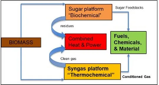
There are two principle and conceptually very different strategies which can be used in the energy conversion of biomass (Figure 1.1).

Figure 1.1- Main pathways for the conversion of biomass into heat, power, fuels and/or chemicals

The first one is the biochemical platform which in turn can be divided in fermentation and anaerobic digestion producing ethanol and methane (not reported in Figure 1.1) respectively. Since it is not an objective of this work, this first pathway will not be further discussed here. A second pathway is the thermochemical biomass conversion that embraces a series of different transformations (not reported in Figure 1.1), ultimately leading either to the production of electricity or other forms of fuels (solid, liquid, gas). Among these possible thermochemical energy conversions combustions, pyrolysis and gasification are quite extensively considered or used in industrial application.

Combustion, one of the most common thermochemical processes, is carried out though high-temperature exothermic oxidation in an oxygen-rich environment. Pyrolysis can be either

(17)

17

fast or slow. The former involves rapid heating in the total absence of oxygen, aiming to maximize the conversion of biomass toward liquid fuels while slow pyrolysis (torrefaction) can be used alternatively to optimize the chars fraction. Differently from combustion, gasification usually operates at lower temperature under sub stoichiometric oxygen condition with the final aim of producing a mixture of gas compounds (mainly CO and H2) known as synthetic gas.

Among the various types of biomass, the biogenic carbon feedstock, such as refuse derived fuels (RDF) generated from municipal solid waste (MSW), has a great potential for contributing to biofuels production as well as green chemicals for industrial applications [8]. The increasing world population, combined with the massive economic growth in developing countries such as India, China and Brazil, is making of municipal solid wastes an increasing concern at a planetary level. In this context, the management of the MSW life cycle will require significant efforts to be tackled whilst also an utmost opportunity to valorize. The lack of suitable space for landfills combined to the hardly biodegradable nature of some of the materials found in MSW calls for supported measures in the upcoming years [9].

According to a 2012 World Bank report [10], production of MSW is estimated to be approximately 1.3 billion tonnes yearly and is supposed to increase to 2.2 billion tonnes yearly by 2025. Most of it is landfilled or ultimately incinerated. The former solution presents several economically and environmentally drawbacks such as:

- The considerable production of CH4, CO, CO2 (high GHG impact). - Potential contamination of groundwater by leachate

- Unpleasant odors

- The massive use of land that could be used for other purposes

- The intrinsic negative cost deriving by a proper management of wastes and respect of safety regulations.

Alternatively to landfilling, MSW can be burnt directly to generate heat and electricity. This technique has been used extensively in many developed countries mainly because of its high potential for energy recovery. Over the last decades incineration has been proposed as the most convenient technology to reduce MSW volume since it is a relatively simple technology, well known and mastered, that can reduce the initial volume of waste by as much as 85% whilst offering solutions for problems such as waste odor and leachate. However, in

(18)

18

the last decades, the incineration primary objective of reducing the generated volume of urban waste was edged by new environmental requirements. In fact, new and more restricting policies (Kyoto Protocol, the deliberations at Copenhagen in 2009 and the Landfill Directive of the European Union) were approved, aiming to minimize the environmental impact of atmospheric emissions, risks for human health and to accomplish national/international mandates for energy process recovery. Despite the consistent development of Municipal Solid Waste Incineration (MSWI) technologies as well as Air Pollution Control (APC), some drawbacks and negative impacts still remain, as shown by several recent studies and scientific reports [11]. MSWI exhaust gas produces a multitude of pollutants which are difficult and very costly to keep under control due to the large variability of chemical compounds originally present inside urban feedstock. Moreover, production of MSW is highly subjected to the specific demography of each country which, in addition to other factors, can further impact on its final composition. A concern shared by most of MSWI technologies is that very harmful compounds can be trapped inside micro flying ashes. This can have possible environmental and health consequences on the surrounding area. Besides, other technical issues such as corrosion of the incineration systems have led to a relatively low economic and energy efficiency.

In this context, gasification represents a very promising technology which, so far, has been widely applied to coal but more rarely to biomass and even less to MSW [12]. Lately, the application of this technology to MSW attracted a strong interest as a consequence of recent policies to tackle climate change and natural resources conservation [13]. As a “novel” waste-to-energy technology, gasification has several potential benefits over traditional incineration, mainly related to lower emissions and more flexible and efficient utilization of MSW chemical energy. The first and probably greatest strength of gasification is its environmental performance, since emission tests indicate that gasification meets the existing pollutants limits while having an important role in the reduction of landfill disposal [8]. The second and huge strength of this thermochemical pathway relies in the numerous downstream possible technologies converting syngas and allowing a broad diversity of end products (Figure 1.2).

(19)

19

Besides the aforementioned advantages, gasification also presents other key aspects over combustion technologies. In fact, gasification can use low-value feedstocks and convert them not only into electricity, but also into liquid and gaseous fuels that can be easily handled and transported, with low operational costs [1]. The syngas generated from gasification can also be used in advanced technologies such as gas turbines and fuel cells, with high energy efficiency [14]. When used in combined cycles for heat and power generation, the use of syngas allows for a more efficient removal of species such as sulfur and nitrogen which ultimately results in much lower emissions [15].

Nevertheless, economics must be considered as a fundamental aspect affecting the profitability at commercial scale and ultimately the possibility for a concrete market penetration. This validity has to be proven for MSW gasification [16]. The main economical drawbacks are linked to the operational and capital costs estimated to about 10% higher than those of conventional combustion-based plants [13]. This is mostly due to the ash melting system and the overall higher complexity of the technology.

The gasification process takes place in the gasifier unit where the thermochemical decomposition stages of carbon-based feedstock occurs. Gasifiers are classified mainly on the basis of their gas-solid contacting mode and gasifying medium, ultimately resulting in different architectural and functioning concepts (Figure 1.3). More details about these type of concepts are reported in the next chapter of this work.

(20)

20

Figure 1.3 – Various concepts of gasifier units based on different gas-solid contact modes [17]

In this work, we focused on fluidized beds, being the one operated by the industrial partner (Enerkem)* for biofuels production. More specifically, among various types of fluidization regimes (Figure 1.3), Enerkem adopts the bubbling fluidized bed technology. Based on this hydrodynamic regime, the gasifier unit presents two contiguous regions which can be distinguished based upon different multiphase properties and reactions involved. More specifically:

 The “bubbling bed”, located at the bottom part of the gasifier involves a multiphase environment with reactions between the carbon based feedstock, the inert bed material (heat carrier) and the gasifying agent (steam, and/or air, and/or oxygen);  The “free-board”, located up above the bubbling bed, where the primary syngas

(permanent gas plus tars) are present along with a low concentration of fine particles (char, flying ashes). Part of present tars undergo a process of thermal reforming inside this vessel, ultimately leading to more permanent gas.

The gasifier unit is part of a broader technology (Figure 1.4) and it is used to produce a syngas that is downstream converted to biofuels and green chemicals.

* “ Enerkem’s disruptive technology converts non-recyclable municipal solid waste (i.e. garbage) into cellulosic ethanol, methanol and other renewable chemicals, with better economics and greater sustainability than other technologies relying on fossil sources. Enerkem operates a full-scale commercial facility in Edmonton, Canada as well as both a demonstration plant and a pilot facility in Quebec. The company is developing several cellulosic ethanol and methanol production facilities in North America and globally, based on its modular manufacturing approach.” [18]

(21)

21

Figure 1.4 From MSW to Biofuels - Enerkem overall technology scheme [18]. In the spotlight the first technology stage called fluidized bubbling bed gasifier

The optimization of this type of process at industrial scale is fairly challenging since it involves a complex chemistry as well as mass and energy transfer phenomena in a multi-phase fluid-dynamic environment [19]. In order to limit expensive iterative hands-on experimental work, Computational Fluid Dynamic (CFD) modeling represents a very valuable tool to predict the evolution of fluid-dynamics and thermochemical variables resulting from various design configurations and variations [20]. The possibility of relying on numerical predictions can be very important in a context of technological optimization. Gasification is a well-known process in literature since it has a long tradition of applications in various fields [21]. However, reliable and comprehensive CFD characterization of this process is very challenging and still to be reached. The lack of numerical modeling of gasification is due to the difficulty of accounting for the several thermochemical and fluid dynamic aspects involved in the process combined with the limited computational power which is still representing a major constraint. Despite these limitations, CFD can potentially provide essential information about syngas composition and sensitivity with regard to operating conditions and feedstock properties. The contribution that could be given by simulation analysis may help designing new efficient generation units with significant save of time and money (Figure 1.5).

Gas IN Feedstock IN

Gas OUT Gas-solid Bubbling bed

(22)

22

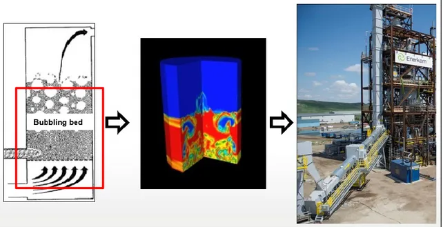
Figure 1.5 - CFD simulations to investigate bubbling fluidized bed and support technology advancement of industrial units

It has been proven that fluid dynamics impacts significantly on the overall efficiency of gasification [20]. This consideration highlights the importance of understanding gasification fluid-dynamics over a continuous space-time thus motivating the objective of this work. In light of this last considerations a “cold” laboratory scale bench reactor was used to reproduce and investigate the fluid dynamics of a gas-solid fluidized bubbling bed. Based upon this lab-scale setup, different CFD models were then implemented and studied. The final target is to apply these CFD models to production scale using them as supporting tools for the designing process and optimization to ultimately improve the overall gasification efficiency. Such improvement may derive from CFD simulations of different design configurations for the gasifier and its operating conditions.

The research was carried out aiming to achieve a reliable numerical description of fluidized bubbling bed technology while finding the advantages and disadvantages specific to each type of numerical model in the perspective of their possible application to industrial scale. Is there a model that could be more efficient to simulate a full industrial scale gasifier and eventually at which cost?

(23)

State of art: numerical modeling applied to multiphase granular systems

23

2. STATE OF THE ART

2.1 GASIFICATION TECHNOLOGY OVERVIEW

Gasification systems present the coexistence of different biomass thermochemical conversion stages such as combustion, pyrolysis and gasification (Figure 2.1). Among various factors, the oxygen availability within the bed is of a primary importance in determining which and where each of these stages takes place. These stages, accordingly to the specific type of technology, may occur separately in the different zones of gasifiers or more spatially homogenized throughout the whole bed.

Figure 2.1 - Gasification of biomass: principal steps and products involved in the thermo-chemical decomposition of biogenic carbon from MSW [22]

Based upon the type of contact between solid material (either biomass, char or inert material) and gas phases (gasification agents and gas released from thermochemical decomposition of

(24)

24

feedstock) different reactor concepts have been developed and applied to gasification of carbon based feedstock [8]. Among several different possibilities in terms of reactor architectures and functioning a significant distinction can be found in moving bed on one side and fluidized bed technology on the other.

In the moving (packed) bed, the feedstock occupies between 30% and 80% of the reactor volume and is supported on a grate. The biomass is fed from the top and it decomposes while it slowly moving downwards the reactor. The ash extraction is made at the base of the bed. Biomass residence times are quite long, usually 2-10 hours. Fairly distinct zones are established in the bed corresponding to the different stages of the gasification process, each at different temperatures. While biomass moves downward, the gasifying agent can flow through the bed concurrently, counter-currently, or cross-wise, which ultimately defines three corresponding types of moving bed concepts namely downdraft, updraft and cross draft beds (Figure 2.2). More details about constructions technology, operating conditions and features of these various fixed beds configurations can be found in [8].

Figure 2.2 – Packed bed gasifiers: a) updraft, b) downdraft, c) cross-draft [8]

In the second type of concept (fluidized systems) the solid particles are kept in a semi-suspended condition (fluidized state) by the flow of the gasifying medium through them at the appropriate velocities [8], which is obviously considerably higher than in packed beds. Biomass is fed usually from the side and near the base of the reactor while the gasifying agent (air, oxygen, steam or CO2) flows upwards (Figure 2.3). The biomass residence times are short, usually seconds or minutes with an extremely efficient mixing due to the high turbulence, so that distinct zones are not established in the bed. All gasification stages occur

(25)

25

simultaneously throughout the bed. Temperatures are highly uniform, typically at 800-1000°C.

Figure 2.3 - Schematic of a fluidized bed gasifier [23]

2.2 FLUIDIZED BUBBLING BED DYNAMICS

There are actually many possible fluid dynamics regimes that could take place inside a fluidized bed gasifier reactor (Figure 2.4). These regimes mainly depend upon the superficial velocity at which the gasifying agent is operated. The actual Enerkem technology is based on an intermediate regime, which is bubbling fluidization (marked in red in Figure 2.4). In this regime, the multiphase system includes regions with very low solids density (called bubble phase), and other regions with a higher solid concentration (called emulsion phase). Bubbles tend to rise through the bed increasing turbulence and increasing the mixing inside the reactor. This ultimately helps to enhance the overall efficiency. For this reason, it is essential to understand bubble fluid dynamics in order to optimize the whole process.

(26)

26

Figure 2.4 - Different fluid-dynamic regime taking place inside a gasifier as function of increasing superficial velocity [24]

Fluidized bed reactors are extensively used both in combustion and gasification systems to thermo chemically convert the solid fuel (and the intermediate pyrolysis products, char and tars) using oxidizing agents and inert bed material. The experience built over decades in this field has shown that bubbling fluidization regime is one of the best ones to guarantee optimal mixing between various phases, ultimately allowing efficient heat and mass transfer [20], [25].

The hydrodynamic behavior of a bubbling fluidized bed results from the balance of forces established between the fluidization agent and the solid particles as well as the mutual repulsive forces arising from particle collisions. In the fixed regime, the equilibrium between the drag force (exerted by the fluidization medium), the constraint reaction offered by the particles (which are packed) and the gravity (acting on the mass of solid particles) ensures a static condition for the bed. In this circumstance, any increase of air velocity results in a linear increase of gas pressure drop until this latter equal the bed weight. A further increase in air velocity leads to a visible bed expansion and to macroscopic instabilities. The transition between the static and dynamic bed regime is marked by the minimum fluidization velocity (Umf). Once this value is exceed, bubbles start forming in the proximity of the injection zone and then move upwards, contributing to phase mixing and turbulence.

In general, fluidization is significantly impacted by the properties of solid particles, which have been classified according to Geldart [26]. This classification, widely accepted in

(27)

27

fluidized bed modeling, divides particles in four groups according to their physical properties and behavior in fluidization system (Figure 2.5).

Figure 2.5 – Graphical representation of Geldart classification, showing the particles behaviors in fluidized systems according to their physical properties [27]

As far as this study is concerned, particles belonging to Group B (namely having a medium diameter in the 40-500 μm range, and density between 1400 and 4000 kg/m3_{) will be the} center of experimental interest. The use of these particles allows reaching good fluidization when operating at high flow rates, while also ensuring bubbles generation on fluidization onset and coalescing during the motion.

All transfer phenomena involved in bubbling fluidized beds, especially in their application to thermochemical processes (such as gasification), are conditioned by the particular type of contact between the various phases [28]. In order to maximize the contact between phases and consequently their mass and heat transfer, a vigorous and turbulent mixing is highly desirable. This mixing is mainly promoted by bubbles motion which, moving inside an emulsion of solid and gas phase [29], enhances their contact and ultimately the transfer phenomena efficiency. Consequently, over the last few decades, significant efforts were invested to cope with a lack of understanding that led to difficulties in design and scale-up of gas-fluidized bed systems [28].

(28)

28

2.3 NUMERICAL MODELING AND MULTI-LEVEL SCALES IN

GAS-SOLID FLOWS

Along with the increasing computational power of the new computers generation, numerical simulations became a very useful tool to investigate fluidized beds. As explained by Van der Hoef et al [28], simulations can be used in two different manners. First they can contribute to bring an insight into the fundamentals of the complex dynamics of particles-gas systems, unveiling the effect of physical principles such as drag, friction, dissipation etc. In addition, they can be used as a predictive tool for supporting the scale-up design of bubbling fluidized beds. As reported by the authors, it is not possible to achieve all of this with one single simulation method but rather with a family of approaches, working on different scales and time lengths, which will be presented in the following of this chapter.

Nowadays Computational Fluid Dynamics (CFD) is the most widespread numerical analysis for such applications and current limitations to their validity are related to theoretical issues as well as CPU performances. In this sense, major constraints are shown very clearly when attempting to simulate real systems, involving complex geometries and physical phenomena, at full industrial scale [20]. Moreover, the time required for CFD simulations increases exponentially with the complexity of the real system under investigation, which represents an additional limitation. In spite of these intrinsic barriers, reliable CFD models are essential for the optimization of fluidized beds. Several information can be derived from post-processing of CFD results, such as the local inert material concentration in bed, fuel mixing efficiency, temperature profiles of solids and gas phases present in the bed, heat flux etc. It would be otherwise impossible to gain a full detailed map (in time and space) of all these variables from the experiments.

Modern CFD is a combination of fluid dynamics models, solved with numerical methods and algorithms applied to fluid flows [20] (or multiphase flows like in the current case of study). The framework within which CFD modeling attempts to describe thermochemical processes, such as gasification, comprises a wide range of physical and chemical interconnections as shown in Figure 2.6.

(29)

29

Figure 2.6 - Modeling of physical and chemical processes interaction in thermochemical conversion of fuels [19]

This complexity derives from the contingent need to account for several aspects involved in multiphase systems and related thermochemical processes, resulting in a fully coupled system of equations. Equations coupling derives, for instance, from several “source terms” which account for the connections between various phases both in terms of exchange of momentum, mass and energy. Another example of equations coupling comes from the phase densities, used in the continuity and momentum equations, in general linked to the system temperature which is retrieved from the energy balance equations.

The theoretical knowledge of the specific type of applications/problems is absolutely fundamental to choose the most appropriate modeling strategy in order to possibly simplify this great complexity. This is also the reason why CFD literature [20] of fluidized bed applications is divided in three main branches based upon the specific part of the reactor under investigation (where the concentration of secondary phase is significantly different) which are principally:

 The bubbling bed  The splash zone  The free board/riser

(30)

30

As far as the actual work is concerned, the focus will be on the first part of the gasifier (the bubbling fluidized bed), whose modeling approaches and inherent literature review will be presented in the rest of this chapter.

The term “bubbling” refers to the specific type of fluid dynamics taking place inside the reactor (Figure 2.4). The choice of this particular system, as mentioned previously, is related to turbulent mixing and high efficiency in term of heat and mass transfer, which justifies its extensive use in the industry. Moreover, when compared to more vigorous regimes (Figure 2.4), the risk of an excessive entrainment of solid particles in the free board and ultimately out of the reactor itself is significantly reduced.

In the industrial bubbling gasifiers, there is always a coexistence of several phases involving both gases (gasification medium combined with the one produced from the thermochemical decomposition of feedstock) and solid particles. A vast majority of these particles are forming the so called “inert bed material” that served the purpose of transferring heat to the fuel particles (in mass less than 10 % of the bed) acting as a thermal buffer.

In cold bubbling applications (usually not employed for industrial purposes) this distinction remains, even though the multiphase system is quite simplified since only two phases can be theoretically involved. Here, ambient air or nitrogen are usually chosen to fluidize the bed, and are considered as primary phase, while the secondary phase involves the solid inert particles. The concentration of the two phases cannot be predicted a priori, being the result of a random event brought by the turbulent mixing caused by bubbles. Solid phase concentration can reach high values in the lower and lateral (close to the wall) areas of the bed, depending on the particle distribution and shape, and low values in the presence of bubbles or close to the bed surface (where bubble explosions occur).

The gas phase is usually modeled according to micro- to macro-scales where a scale length is characterized by the local Knudsen (Kn) number. This number defines the ratio between the mean free path of molecules and a characteristic length scale of the flow. Depending on this number, three regimes and corresponding transitions may be possible. The lowest Knudsen numbers (smaller than 0.01) are representative of incompressible flows that can dynamically be described by the Navier Stokes equations. At the opposite, a Kn higher than 10 would be representative of a free path system where molecules would move freely and colliding only with the system boundaries. These two extreme situations for the gas phase

(31)

31

find a modeling correspondence in the continuum and molecular models. While this latter can apply only to micro-scale (despite being theoretically applicable to any length scale, its use is limited by computing capacity) the former is used to wider scale systems (in the order of meters) investigation. The gap between the two models is filled by the kinetic theory based on the Boltzman equation [28].

As for the solids there is a possibility to define various types of models accordingly to the scale of simulations and particles density magnitude. Some of the methods used to describe granular systems are taken from the molecular gas theory and extended for analogy to fit the need to describe particles properties that are obviously quite different. Solid particles and gas molecules do not share the same mechanical properties. Specifically, it happens that while molecules can be assumed to collide elastically (with no loss of kinetic energy during the collision), real particles collisions involve a surface friction and elastic-plastic deformations, which generate a loss in the kinetic energy of solid system. These two last aspects can distance the granular flow behaviour from ideal gas one quite significantly making the description of the solid particles system not straight forward. From this point of view, the granular flows description and modeling is quite complex but at the same time presents also a significant margin of improvement towards reliable hydro-dynamic models development [28]. When choosing the proper model for a multiphase system, a very important aspect to consider is the degree of particle packing inside the bed. Depending on this value, various interphase coupling possibilities are available, as reported by Elgobashi [30] and shown in Figure 2.7.

(32)

32

Given the high density of solids involved, the four-way coupling (Figure 2.7) was considered for current thesis work. In fact, in bubbling fluidized beds, the solid fraction ranges from 0 (in presence of pure gas bubbles) to a maximum packing limit that in case of irregular shape particles is a phase fraction ranging between 0.5-0.6. In such circumstances, the solid concentration can drastically affect the gas pattern and structure while particles are interacting with each other (and with the boundaries of the physical domain) exchanging momentum throughout collisions and surface friction.

In bubbling fluidized beds with no chemical reactions, the two main protagonists driving the fluid dynamic of the overall system are the fluid-particles drag forces and the particle-particle interactions.

In the last decades, despite the technological advancement in computing science, the construction of reliable models for large-scale systems has been seriously hindered by the lack of understanding of the fundamentals of dense gas-particle flows [31]. As remarked by Van der Hoef et al. [28], one very big challenge, studying multiphase systems, is represented by the definition of spatial scales involved. In general the accepted concept is that larger flow structures (in the order of meters) might be affected by smaller scales where particle-particles interactions take place. This considerations can explain why many efforts have been put forward over the years to search for proper micro to meso-scale modeling equations of gas-particle and particle-particle interactions. These interactions at small scale are of utmost importance since they allow developing proper closure laws which, once applied at macroscopic scale, provides better modeling of macroscopic flow structures, which are usually of major industrial interest. Open literature [20] reports that there are currently three main techniques to investigate the multiphase fluidized systems whose multi-level scheme and inter-connections are depicted in Figure 2.8.

(33)

33

Figure 2.8 - Multi-level modeling scheme [28]

From the smaller to the larger scale we can find:

1. Lattice Boltzman Model (LBM) or alternatively the Discrete Numerical Simulations (DNS) (which represent a broad family of methods despite being not reported in Figure 2.8).

2. Eulerian-Lagrangian Discrete Particle Model (DPM). Belonging to this family are the Kinetic Theory of Granular Flow (KTGF) model (used in this work), the hard/soft sphere models and the MPIC approach.

3. Eulerian-Eulerian Two Fluid Model (TFM).

2.3.1 Principle features of different numerical approach to solid-gas flows At the smallest applicability scale (Figure 2.8) is the Lattice Boltzman Model (LBM) which in the last two decades, has emerged as a promising tool for modelling the Navier-Stokes equations and simulating complex fluid flows [32]. The fundamental idea is that gases/fluids can be imagined as consisting of a large number of small particles moving with random motions. The exchange of momentum and energy is achieved through particle streaming and billiard-like particle collisions. More details about the mathematical derivation and formulation of this method can be found in works of Bao and Meskas [32] as well as in Van der Hoef et al [28]. Alternatively to LBM there is another class of methods called Direct Numerical Simulation (DNS). This family of methods are the most detailed approach, fully resolving the flow around each single particle (Figure 2.9) by solving the Navier Stokes

(34)

34

(N.S) equations without turbulence models. The solid-fluid interaction is based on a “stick” boundary conditions at the particle surface site enabling to describe a fully resolved momentum exchange between phases. In such type of simulations, turbulence swirls and their effects are accounted in the whole range of time and space scale length making this approach highly computationally demanding. In turbulent flows, the total energy is consumed according to a macro to micro scale of vortex (also known as Kolmogorov scale) induced by turbulence and their correct numerical resolution would require to account and solve for the whole scale of these vortex. Specifically, it can be proved that the ratio between the Kolmogorov micro-viscosity scale (for which N.S equations have to be solved) and the macro scale (comparable to the length of the flow field) is scaling up with 1/Re, ultimately resulting in extremely fine numerical mesh required to study flow field at high Reynold numbers.

Figure 2.9 – Example of a Direct Numerical Simulation (DNS) where the gas flow is numerically resolved around each single particle in a system [33], [34], [35]

As an example, a simulation of a flow with a Re∼106 _{in a field of ∼1 m would require to} work on a numerical grid in the order of 10-5 _{m. For this reason DNS has been used to} describe only very small scale systems (around 1 cm max) comprising few thousand particles [28]. Even with the most powerful new generation computers, this method is not reported in literature among those potential techniques used to study multiphase applications at pilot or

(35)

35

industrial scale [20]. The goal of these simulations is rather to develop and tune drag laws that might possibly be employed in larger scale applicability models (DPM , TFM etc..). In their recent work Tang et al. [36] used a DNS approach to study the fluidization of 5000 particles in a pseudo-2D gas-fluidized of 3.75·10-4_m3_{. Using Particle Image Velocimetry} (PIV) they were able to obtain detailed information on the gas flow and motion of individual particles, with specific focus on comparing the empirical and numerical particle granular temperature (as key characteristics of particle velocity fluctuations).

The empirical system investigated in the present thesis work, comprises a total volume of approximately 1.85·10-2_m3 _{with around 680 million particles. It is here clearly evident how} a DNS approach would not be possible to characterize such a dense particle system.

The other two modeling approaches, namely the TFM and DPM (DDPM)-KTGF, were used in this work to investigate bubbling bed fluidization. The decision of investigating these two models was motivated by their conceptual difference in the numerical treatment of the solid phase. From here, the motivation in exploring the main features of these two CFD models to ultimately determine and compare the advantages and drawbacks of each of them in the perspective of their potential application to industrial scale. The most significant features of these two methods and related applications to multiphase systems (as reported in open literature) are presented in the rest of this chapter while their proper equations will be shown in Chapter 3.

The DPM (DDPM)-KTGF represents only one of the possible options in the Eulerian-Lagrangian description of gas-solid systems (where the hard or soft sphere approaches may also be used). The reasons behind the choice of this particular Lagrangian approach will be discussed at the end of section 3.3.

The two selected modeling approaches share a very important aspect, which is the Kinetic Theory of Granular Flow (KTGF) [37], [38] used to define the granular properties of the solid phase. According to this theory, the particles behavior is approached in a similar manner to the one of a molecular gas. The use of this theory allows to bring important closure relations ultimately bridging the micro-scale description of granular flows (DNS) to a macro scale approach. According to the KTGF theory, two granular flow variables such as the solid pressure and the solid shear stress tensor (both including kinetic, frictional and collisional components) are introduced to account for repulsive forces between colliding particles.

(36)

36

These two variables are in turn computed as a function of the local granular temperature (for which an extra conservation equation is solved) which is defined from the fluctuations in the velocity of the solid particles. More explanation of each of these term can be found in the next chapter (section 3.3).

The Euler-Lagrangian Discrete Particle Model (DPM) represents a class of methods occupying an intermediate place in the applicability scale shown in Figure 2.8. In DPM methods, the primary phase (gas/fluid phase) is described as a continuum (fluid) by solving the Navier Stokes equations, while to the secondary (solid) phase is modeled a system of spheres according to a discrete approach. Differently from the DNS approach, the cell size over which the gas field is resolved contains many particles and the flow properties are averaged within each cell resulting in the impossibility to detail the gas flow around each particle. However the advantage of this method is the possibility to provide a detailed description of the overall solid phase distribution inside the domain (thanks to the Lagrangian particles tracking) without confining the study to only few particles (as for the DNS approach). In this context the trajectory of each sphere results from a double integration of the Newton’s second law which expresses a force balance applied to each of them within the Lagrangian framework. Consequently this class of methods allows detailing the motion and evolution of feed stock solid particles in the bed (for hot model applications) as well as simply investigating cold segregation phenomena (shown as an example in Figure 2.10) when particles of different size are used.

(37)

37

Figure 2.10 -Snapshots of size segregation in fluidized bed: (a) simulated and (b) experimental binary mixture mixing [39]

In order to avoid any possible confusion about the nomenclature (acronym) of the Lagrangian model used in this work (where DKTGF will be used in place of DPM-KTGF), it is important to highlight some aspects which strictly relate to the definition of this type of model within the software used here (Fluent). According to the present software, the DPM approach will only be valid when the solid fraction of the dispersed phase (solid particles) is below 10-12% of the fluid (gas) domain [40]. In such a circumstance the volume fraction of the discrete phase is sufficiently low and it is not taken into account when assembling the continuous phase equations. Moreover the low volume fraction of particles allows neglecting the particle-particle interactions (collisions), which represent a significant simplification. However the respect of this solid load threshold limits the exploitation of the DPM approach (so conceived) to bubbling fluidized bed application. In such a type of system, particles can accumulate very easily (in some part of the bed even exceeding the 50

(38)

38

% of the total volume) requiring to both account for the volume exclusion effect in the primary phase (considering a gas fraction coefficient in both the continuity and momentum equations) and particle-particle collisions. For these reasons a Dense Discrete Phase Model (DDPM) was used in this work and coupled with the Kinetic Theory of Granular Flow (KTGF) to account for particle-particle interaction forces. While the DPM represents a class of Lagrangian approaches to multiphase flows (well known in open literature and independent from any software nomenclature), this DDPM approach comes as an extension of the DPM to high density granular systems according to the definitions specific of the present software. Therefore in the rest of this work, the acronym DDPM will be used instead of DPM, which will also allow to be consistent with other works found in open literature where authors used the same software and referred to the DDPM approach.

In the DDPM-KTGF model, particles contact forces (collisions) are estimated by solving the gradients of granular flow variables (solid pressure term and shear stress tensor), which are derived from an averaging process involving the position and velocities of particle over the Eulerian grid (where the primary phase is solved). Conversely, in fully resolved collisional methods (such as the Eulerian-Lagrangian soft sphere model briefly introduced at the end of section 3.3) collisions are independent of Eulerian variables but are rather computed as a function of particles mechanical properties (elasticity coefficient, particle stiffness, damping coefficient etc..). This motivates the reference to this DDPM-KTGF as an Euler-Lagrangian hybrid approach to multiphase system [41].

At a larger applicability scale (see Figure 2.8) there is the Eulerian-Eulerian Two Fluid

model (TFM) which considers a simplified description of both gas and solid phases. These

are both described as inter-penetrating fluids, thus introducing phasic volume fraction as continuous function of space and time. The summation of all phasic volume fraction is obviously equal to one. The application of this method to multiphase granular systems allows observing the concentration of different phases within the domain thus without recognizing the single particles distribution (Figure 2.11). Despite the apparent simplicity in the representation of various phases, this one of the most complex approach to multiphase granular systems since it requires the definition of several constitutive relations (derived from the application of the KTGF theory) to close the set of governing equations. These latter are represented by the mass and momentum conservation equations, which are solved

(39)

39

per each phase. The resolution of these equations allows to recover the motion field (velocity and pressure) for both phases together with the distribution of phasic fractions.

This method proved to be computationally cost-effective when the volume fractions of gas and solid phases are comparable and the interaction between these phases is significantly impacting on the overall fluid dynamic behavior such as in bubbling fluidized beds [20]

As a sum up of these three different class of methods, namely the DNS simulations, the DPM approach and the TFM, Figure 2.12 schematically reports the main differences and scales of applicability. Here is provided an example of multi-level modeling application to the study of a life-scale fluidized bed (left). The arrows represent a change of model. In first place the TFM (see enlargement) can be used to simulate large sections of the unit providing overall information about phase concentrations (see the shade of gray cell by cell). On the right, a part of the same section is modeled using discrete particles (DPM). The gas-phase is solved on the same grid as in the two-fluid model which is containing a certain number of particles whose shape or size is not relevant in capturing the gas flow patterns and features. The bottom graph shows the most detailed level, where the gas-phase is solved on a grid much smaller than the size of the particles (DNS) which allows to account for the specific particles properties (size, shape etc..) and their effect on the gas flow.

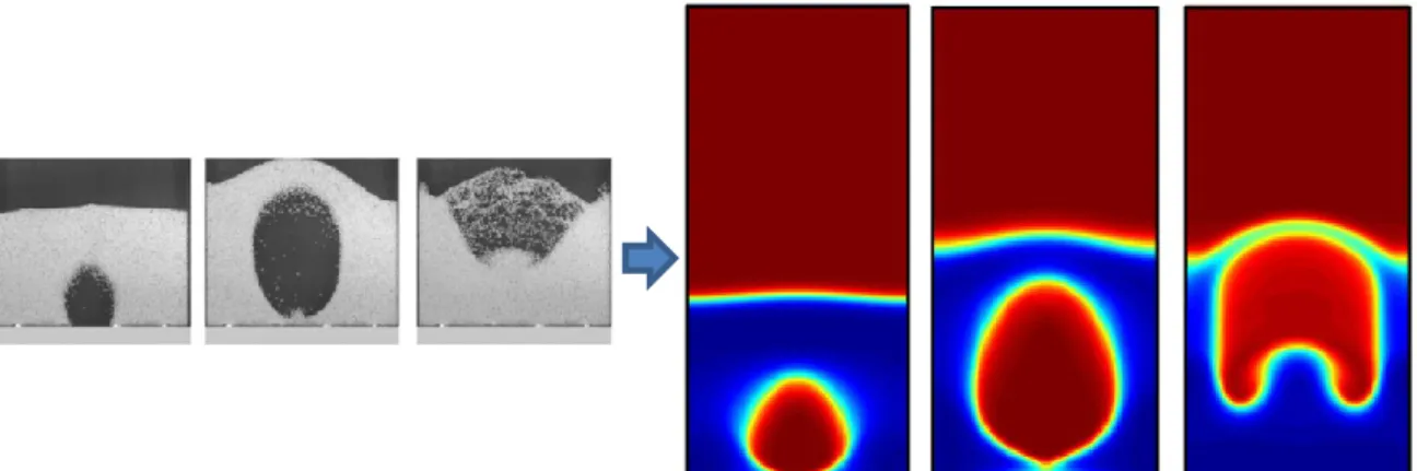
Figure 2.11 - Injection of a single bubble into the center of a mono-disperse fluidized bed consisting of spherical glass beads of 2.5mm diameter at incipient fluidization conditions. Comparison of