Development and testing of scaling laws for fluidized beds

DEVELOPMENT AND TESTING OF SCALING LAWS FOR FLUIDIZED BEDS

by

MARK THOMAS NICASTRO

B.S.M.E., Rensselear Polytechnic Institute (1980)

SUBMITTED TO THE DEPARTMENT OF MECHANICAL ENGINEERING IN PARTIAL

FULFILLMENT OF THE REQUIREMENTS FOR THE

DEGREE OF MASTER OF SCIENCE IN MECHANICAL ENGINEERING

at the

MASSACHUSETTS INSTITUTE OF TECHNOLOGY June 1982

Massachusetts Institute of Technology 1982

Signature redacted

Signature of Author... '* .. .

.v.

Department of Mechanical Engineering April 8, 1982

Signature redacted

by..

Signature redacted

by...

Archives

JUL 30 1982

-2-DEVELOPMENT AND TESTING OF SCALING LAWS FOR FLUIDIZED BEDS

by

MARK THOMAS NICASTRO

Submitted to the Department of Mechanical Engineering on April 8, 1982 in partial fulfillment of the requirements for the Degree of Master of Science in

Mechanical Engineering ABSTRACT

Scaling laws were developed which allow a fluidized bed operating under one set of fluid conditions to be modeled by another bed operated with different fluid properties.

The scaling laws were verified by comparing measurements made in an atmospheric fluidized bed combustor operating at 1050 K and its

scale model operating at ambient conditions. The tests showed that both beds had similar fluid dynamic behavior as measured by minimum fluidizing velocity and pressure fluctuations caused by bubbles. These results were consistent with the predictions of the scaling laws.

The results indicate that the scaling laws can be used to accurately construct a scale model of a fluidized bed that exhibits fluid dynamic characteristics which are related to the characteristics of the full size

bed by known scale factors. In this way the model bed can be used to pre-dict the behavior of the full size bed.

Thesis Supervisor: Dr. Leon Glicksman

-3-ACKNOWLEDGEMENTS

My thesis advisor, Dr. Leon R. Glicksman, is credited with the

de-velopment of the scaling laws and I would also like to thank him for his guidance and insight throughout this project. Special thanks are in order for Dr. Peter M. Walsh for allowing me to conduct my experiments at the Fluidized Combustion Research Facility. His hard work in operating the combustor and gathering data, and his generously donated time for expert consultation is sincerely acknowledged.

The advice and enlightenment, frequently sought from and patiently provided by my officemates (and friends) was greatly appreciated. Also acknowledged is the excellent technical service provided at both the Combustion Facility and the Mechanical Engineering Shop.

Since one's frame of mind is an'important factor in determining one's work performance, I would also like to acknowledge my officemates and others who created a warm and friendly working atmosphere. Their moral support and that of my parents and my fiancedwas also greatly

appreciated.

The fine job done in typing this manuscript is credited to Sandy Williams.

Finally, the sponsorship of this research by the American Electric Power Company and the Tennessee Valley Authority is gratefully acknowledged.

-4-TABLE OF CONTENTS PAGE ABSTRACT 2 ACKNOWLEDGEMENTS 3 TABLE OF CONTENTS 4 LIST OF FIGURES 6 LIST OF TABLES 12 NOMENCLATURE 14 CHAPTER 1 - INTRODUCTION 17

CHAPTER 2 - THE SCALING LAWS 22

2.1 Deriving the Scaling Parameters 22

2.2 Testing the Scaling Laws 30

2.3 Approximation of Scaling Laws 37

Near the Distributor

CHAPTER 3 - EXPERIMENTAL APPARATUS 42

3.1 The Hot Bed 42

3.2 The Cold Bed 46

3.3 Pressure Fluctuation Probes 50

3.4 Recording and Processing Pressure 54 Fluctuation Signals

CHAPTER 4 - EXPERIMENTAL PROCEDURE 57

4.1 Hot Bed Experiments 58

4.2 Bed Particle Measurements 60

- Particle Size Distribution 60

- Mean Particle Size Based on

Specific Surface Area 61

- Particle Shape Factor Determination 64

4.3 Cold Bed Experiments 68

4.4 Analyzing Pressure Fluctuation Data 74 4.5 Measurement of Minimum Fluidization Velocity 83

-5-PAGE

86 87 CHAPTER 5 - RESULTS AND DISCUSSION

5.1 Scaling Law Tests

- Run No. 1

- Run No. 2

- Run No. 3

5.2 Effect of Solid Feeds on Bed Fluid Mechanics CHAPTER 6

REFERENCES APPENDIX A APPENDIX B

CONCLUSIONS AND RECOMMENDATIONS

- PARTIAL EXPLANATION OF PRESSURE FLUCTUATIONS RECORDED WITH A SINGLE PROBE.

- COMPUTER PROGRAM FOR FINDING MEAN PARTICLE

DIAMETER BASED ON SPECIFIC SURFACE AREA APPENDIX C - RAW DATA FROM SCALING EXPERIMENTS

APPENDIX D - MINIMUM FLUIDIZATION VELOCITY DATA

87 104 115 127 131 135 137 143 152 190

-6-LIST OF FIGURES

NUMBER TITLE _PAGE

3.1 _{Schematic Layout of M.I.T. 0.6 m x 0.6 m, 500 kW 43} (Thermal) Atmospheric Fluidized Combustion

Research Facility.

3.2 _{Hot and Cold Bed Distributor Layout and Nozzle 44} Design (Cold Bed Dimensions are Shown in

Parentheses.)

3.3 _{Hot and Cold Bed Internal Configuration 47}

(Cold Bed Dimensions are Shown in Parentheses.)

3.4 _{Schematic Layout of Cold Bed Laboratory 49}

Apparatus.

3.5 _{Double Probe Design for Measuring Instantaneous 51} Pressure Drop Fluctuations in Hot and Cold Beds.

(Cold Bed Dimensions are Shown in Parentheses.)

3.6 _{Single Probe Design for Measuring Instantaneous 52} Pressure Fluctuations in Hot and Cold Beds.

(Cold Bed Dimensions are Shown in Parentheses.)

3.7 _{Schematic Layout of Instrumentation and Recording 55} System for Hot and Cold Bed Experiments.

4.1 _{Method for Determining Log-Normal Parameters 65} from Cumulative Particle Size Data (from Table

4.1).

4.2 _{Typical Bed Particle Sample Prepared for 69} Circularity Measurement. Size Range: -1000 iim

to +710 -pm.

4.3 Method for Finding Cold Bed Particle Size 71

Distribution from Hot Bed Sieve Analysis Data.

4.4 _{Comparison of Typical Bed Particles Used in 73} Scaling Law Tests.

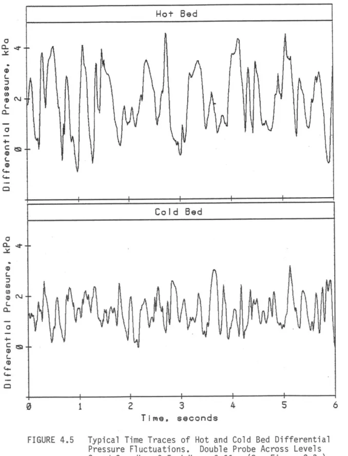
4.5 _{Typical Time Traces of Hot and Cold Bed 75}

Differential Pressure Fluctuations. _{Double Probe} Across Levels 2 and 3; x/L = 0.5; L/Lf = 0.66. (See Figure 3.3.)

-7-NUMBER TITLE PAGE

4.6 Typical Power Spectra of Hot and Cold Bed 77 Differential Pressure Fluctuations. Double Probe

Across Levels 2 and 3; x/L = 0.5; L/Lf = 0.66. (See Figure 3.3.)

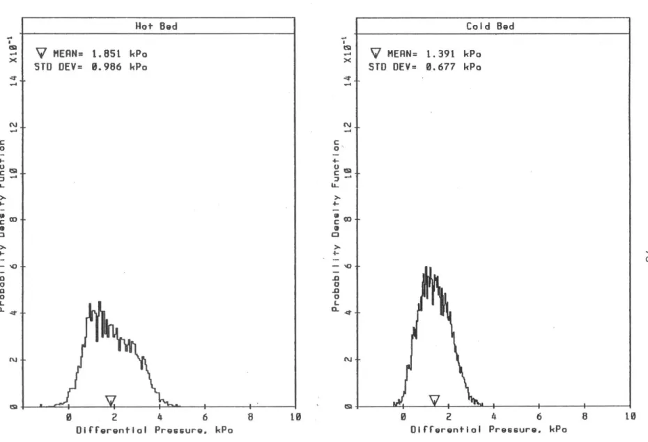
4.7 Typical Probability Density of Hot and Cold Bed 78 Differential Pressure Fluctuations. Double

Probe Across Levels 2 and 3; x/L = 0.5; L/Lf = 0.66. (See Figure 3.3.)

4.8 Method of Quantitatively Comparing Dimensionless 80 Power Spectra of Pressure Fluctuations.

4.9 Power Spectra of Three, 40-Second Samples of 81 Differential Pressure Fluctuations Taken Over a

Period of Ten Minutes to Show the Reproducibility of the Data.

4.10 _{Probability Density of Three, 120-Second Records 82} of Differential Pressure Fluctuations Taken Over

a Period of Ten Minutes to Show the Reproducibility of the Data.

4.11 _{Determination of Minimum Fluidizing Velocity from 84} Measurements of Pressure Drop Versus Gas Velocity

Through the Bed.

5.1 _{Comparison of Dimensionless Power Spectra of 90} Differential Pressure Fluctuations. Run No. 1:

Double Probe Across Levels 2 and 3; x/L = 0.5. (See Figure 3.3.)

5.2 Comparison of Probability Density of Dimensionless 92 Differential Pressure Fluctuations. Run No. 1: Double

Probe Across Levels 2 and 3; x/L = 0.5. (See Figure 3.3.)

5.3 _{Comparison of Dimensionless Power Spectra of 97} Differential Pressure Fluctuations. Run No. 1:

Double Probe Across Levels 2 and 3; x/L = 0.25. (See Figure 3.3.)

5.4 _{Comparison of Probability Density of Dimensionless 98} Differential Pressure Fluctuations. Run No. 1:

Double Probe Across Levels 2 and 3; x/L = 0.25. (See Figure 3.3.)

-8-NUMBER TITLE PAGE

5.5 Comparison of Dimensionless Power Spectra of 99 Differential Pressure Fluctuations. Run No. 1:

Double Probe Across Levels 2 and 3; x/L = 0.0. (See Figure 3.3.)

5.6 Comparison of Probability Density of Dimensionless 100 Diffferential Pressure Fluctuations. Run No. 1:

Double Probe Across Levels 2 and 3; x/L = 0.0. (See Figure 3.3.)

5.7 _{Comparison of Dimensionless Power Spectra of 107} Differential Pressure Fluctuations. Run No. 2:

Double Probe Across Levels 2 and 3; x/L = 0.5. (See Figure 3.3.)

5.8 Comparison of Probability Density of Dimensionless 109 Differential Pressure Fluctuations. Run No. 2:

Double Probe Across Levels 2 and 3; x/L = 0.5. (See Figure 3.3.)

5.9 Comparison of Dimensionless Power Spectra of 110 Differential Pressure Fluctuations. Run No. 2:

Double Probe Across Levels 2 and 3; x/L = 0.25. (See Figure 3.3.)

5.10 Comparison of Probability Density of Dimensionless 111 Differential Pressure Fluctuations. Run No. 2:

Double Probe Across Levels 2 and 3; x/L = 0.25. (See Figure 3.3.)

5.11 Comparison of Dimensionless Power Spectra of 112 Differential Pressure Fluctuations. Run No. 2:

Double Probe Across Levels 2 and 3; x/L = 0.0. (See Figure 3.3.)

5.12 Comparison of Probability Density of Dimensionless 113 Differential Pressure Fluctuations. Run No. 2:

Double Probe Across Levels 2 and 3; x/L = 0.0. (See Figure 3.3.)

5.13 _{Comparison of Dimensionless Power Spectra of 119} Pressure Fluctuations. Run No. 3: Single Probe at

Level 1; x/L = 0.5. (See Figure 3.3.)

5.14 Comparison of Probability Density of Dimensionless 120 Pressure Fluctuations. Run No. 3; Single Probe at

-9-NUMBER TITLE PAGE

5.15 Comparison of Dimensionless Power Spectra of 122 Pressure Fluctuations. Run No. 3; Single Probe

at Level 2; x/L = 0.5. (See Figure 3.3.)

5.16 Comparison of Probability Density of 123

Dimensionless Pressure Fluctuations. Run No. 3;

Single Probe at Level 2; x/L = 0.5. (See Figure 3.3.)

A.1 Idealized Pressure Trace Produced by a Single 138 Bubble.

A.2 Combination Pressure Probe and Light Based 141 Void Detector.

A.3 Traces Produced by Pressure Probe and Light 142 Probe Void Detector.

B.1 Best Fit Log-Normal Distribution Found from 147 Computer Program Using the Sample Data.

C.1 Comparison of Power Spectra of Differential 161 Pressure Fluctuations. Run No. 1: Double Probe

Across Levels 2 and 3; x/L = 0.5. (See Figure 3.3.)

C.2 Comparison of Probability Density of Differential 162 Pressure Fluctuations. Run No. 1; Double Probe

Across Levels 2 and 3; x/L = 0.5. (See Figure 3.3.)

C.3 Comparison of Power Spectra of Differential 163 Pressure Fluctuations. Run No. 1; Double Probe

Across Levels 2 and 3; x/L = 0.25. (See Figure 3.3.)

C.4 Comparison of Probability Density of Differential 164 Pressure Fluctuations. Run No. 1; Double Probe

Across Levels 2 and 3; x/L = 0.25. (See Figure 3.3.)

C.5 Comparison of Power Spectra of Differential Pressure 165 Fluctuations. Run No. 1; Double Probe Across Levels

2 and 3; x/L = 0.0. (See Figure 3.3.)

C.6 Comparison of Probability Density of Differential 166 Pressure Fluctuations. Run No. 1; Double Probe

Across Levels 2 and 3; x/L = 0.0. (See Figure 3.3.)

C.7 Comparison of Power Spectra of Differential Pressure 172a Fluctuations. Run No. 2; Double Probe Across Levels

-10-FIGURE TITLE PAGE

C.8 Comparison of Probability Density of Differential 173 Pressure Fluctuations. Run No. 2; Double Probe

Across Levels 2 and 3; x/L = 0.5. (See Figure 3.3.)

C.9 Comparison of Power Spectra of Differential 174 Pressure Fluctuations. Run No. 2; Double Probe

Across Levels 2 and 3; x/L = 0.25. (See Figure 3.3.)

C.10 Comparison of Probability Density of Differential 175 Pressure Fluctuations. Run No. 2; Double Probe

Across Levels 2 and 3; x/L = 0.25. (See Figure 3.3.)

C.11 Comparison of Power Spectra of Differential Pressure 176 Fluctuations. Run No. 2; Double Probe Across Levels

2 and 3; x/L = 0.0. (See Figure 3.3.)

C.12 Comparison of Probability Density of Differential 177 Pressure Fluctuations. Run No. 2; Double Probe

Across Levels 2 and 3; x/L = 0.0. (See Figure 3.3.)

C.13 Comparison of Power Spectra of Pressure Fluctuations. 184 Run No. 3; Single Probe of Level 1; x/L = 0.5.

(See Figure 3.3.)

C.14 Comparison of Probability Density of Pressure 185 Fluctuations. Run No. 3; Single Probe at Level 1;

x/L = 0.5. (See Figure 3.3.)

C.15 Comparison of Power Spectra of Pressure Fluctuations. 186 Run No. 3; Single Probe at Level 2; x/L = 0.5.

(See Figure 3.3.)

C.16 Comparison of Probability Density of Pressure 187 Fluctuations. Run No. 3; Single Probe at Level 2;

x/L = 0.5. (See Figure 3.3.)

C.17 Comparison of Shape Factor Versus Particle Size for 189 the Different Bed Materials Used in the Scaling

Experiments.

D.1 Data for Determining Minimum Fluidization Velocity. 191 Run No. 1; Hot Bed Tb = 667 K.

D.2 Data for Determining Minimum Fluidization Velocity. 192 Run No. 1; Cold Bed (iron shot); Tb = 298 K.

D.3 Data for Determining Minimum Fluidization Velocity. 193 Run No. 1; Cold Bed (iron grit); Tb = 306 K.

-11-FIGURE TITLE PAGE

D.4 Data for Determining Minimum Fluidization Velocity. 194 Run No. 2; Hot Bed; Tb = 764 K.

D.5 Data for Determining Minimum Fluidization Velocity. 195 Run No. 2; Cold Bed (iron grit); Tb = 297 K.

D.6 Data for Determining Minimum Fluidization Velocity. 196 Run No. 2; Cold Bed (hot bed material); Tb = 298 K.

D.7 Data for Determining Minimum Fluidization Velocity. 197 Run No. 3; Cold Bed (iron grit); Tb = 302 K.

-12-LIST OF TABLES

NUMBER _{TITLE PAGE}

2.1 _{Scale Factors for a Cold Bed Model Operating 34} at 3000_{K to Simulate the Hot Bed Combustor}

Operating at 1050*K

4.1 _{Typical Sieve Analysis Data for a Sample of 62}

Hot Bed Material

4.2 _{Comparison of the Degree of Sphericity and the 67} Degree of Circularity for Five Regular Polyhedra

5.1 _{Values of Scaling Parameters for Run No. 1 88}

5.2 Summary of Results for Run No. 1 101

5.3 Percent Error in Matching Power Spectral 103

Density Functions for Pressure Fluctuations in Hot and Cold Beds. Run No. 1; Double Probe Across Levels 2 and 3 (See Figure 3.3.)

5.4 _{Values of Scaling Parameters for Run No. 2 106}

5.5 _{Summary of Results for Run No. 2 114}

5.6 _{Percent Error in Matching Power Spectral 116} Density Functions for Pressure Fluctuations in

Hot and Cold Beds. Run No. 2; Double Probe Across Levels 2 and 3 (See Figure 3.3.)

5.7 _{Values for Scaling Parameters for Run No. 3 118}

5.8 _{Summary of Results for Run No. 3 125}

5.9 _{Percent Error in Matching Power Spectral Density 126} Functions for Pressure Fluctuations in Hot and

Cold Beds. Run No. 3; Single Probe

C.1 _{Composition and Properties of 23 gal/ton Colorado 153} Oil Shale from the C-b Site in the Piceance Creek

Basin

C.2 _{Composition and Properties of Kentucky No. 9 154} Bituminous Coal

-13-NUMBER TITLE PAGE

C.3 Sieve Analysis and Physical Properties of No. 20 155 Ottawa Silica Sand, Used as Primary Bed Material

in Fluidized Bed Combustor

C.4 Sieve Analysis of Combustor Fuel Feed Particles 157 for Run No. 1

C.5 Sieve Analysis and Shape Factor Measurements of 158 Bed Particles for Run No. 1

C.6 Operating Conditions in Hot and Cold Bed 160 Experiments for Run No. 1

C.7 Dimensional Result of Measurements Taken in Hot 167 and Cold Bed Experiments - Run No. 1

C.8 Sieve Analysis of Combustor Fuel Feed Particles 169 for Run No. 2

C.9 Sieve Analysis and Shape Factor Measurements of 170 Bed Particles for Run No. 2

C.10 Operating Conditions in Hot and Cold Bed Experi- 172

ments for Run No. 2

C.11 Dimensional Results of Measurements Taken in Hot 178 and Cold Bed Experiments - Run No. 2

C.12 Sieve Analysis of Combustor Fuel Feed Particles 180 for Run No. 3

C.13 Sieve Analysis and Shape Factor Measurements of 181 Bed Particles for Run No. 3

C.14 Operating Conditions in Hot and Cold Bed Experi- 183 ments for Run No. 3

C.15 Dimensional Results of Measurements Taken in Hot 188 and Cold Experiments - Run No. 3

-14-NOMENCLATURE

a' specific surface or surface of solid per mass of solid, m2/kg

A cross-sectional area, m2

Aor cross-sectional area of distributor nozzle openings, m2

db _{effective bubble diameter, m}

dor diameter of distributor nozzle openings, m d _{particle diameter, m}

di mean particle diameter based on specific surface area, m p

d P9 mean particle diameter based on mass, m

f frequency, Hz

f frequency of lowest peak in power spectrum of pressure

fluctuations, Hz

g = 9.804 m/s2_{, acceleration of gravity at Cambridge, Mass.}

Ah distance between probe parts, m

KE kinetic energy of flow, N/M2

L length of side of bed, m

LlL2,L3 entire set of dimensions that describes the bed internal

configuration, m

Lf height of a bubbling fluidized bed measured from point where

fluid enters bed, m

m mass flow rate, Kg/s

p particle size distribution function, m~1

P absolute pressure, N/M2 _{or cumulative particle size}

distribu-tion, dimensionless

AP pressure drop or differential pressure, N/M2

-15-AP_ local minimum in differential pressure trace, N/m2 AP mean differential pressure fluctuation, N/m2

Pb absolute pressure at bottom of fluidized bed, N/M

2

APb pressure drop across a fluidized bed, N/M2

APsd standard deviation of pressure fluctuations, N/M2

S velocity slip ratio (velocity of solid divided by velocity of fluid), dimensionless

t time, s

T temperature, *K

Ta temperature of air, *K Tb mean bed temperature, *K

u fluid velocity, m/s

u local bed fluid velocity vector, m/s

ub velocity of a bubble rising through a bed, m/s

umf superficial fluid velocity at minimum fluidizing conditions, M/s

u 0superficial fluid velocity (measured on an empty tube basis) through a bed of solids, m/s

u or velocity of fluid through distributor nozzle openings, m/s v solid velocity, m/s

v local bed solid velocity vector, m/s x distance from probe tip to wall of bed, m

Greek Symbols

6 fraction of fluidized bed consisting of bubbles, dimensionless E: local void fraction, dimensionless

Ef void fraction in a bubbling bed as a whole, dimensionless

emf void fraction in a bubbling bed as a whole at minimum fluidizing conditions, dimensionless

-16-'P viscosity of fluid, kg/m-s p density, Kg/m3

Pb density of fluidized bed (fluid and solid mixture) as a whole, Kg/m3

p 9density of fluid in bed at pressure, Pb and temperature, Tb

9 Kg/m3

por density of fluid entering bed at exit of distributor nozzles,

or Kg/m3

pS density of bed solids, Kg/m3

a parameter of log-normal distribution function (geometric standard deviation), dimensionless

time required for bubble passage, s

circularity of a bed particle, dimensionless mean circularity of bed particles, dimensionless

c

$s sphericity of a bed particle, dimensionless Superscript

-17-CHAPTER 1 INTRODUCTION

In the midst of an energy emergency, those alternative energy sources which can be made available in the next decade are of prime importance. Coal, being this country's most abundant energy resource, seems a likely candidate for making us energy independent. Unfortu-nately, finding ways to use coal cheaply and cleanly has been a diff-cult task. However, fluidized beds show potential for being able to utilize coal as an energy source in new coal combustion, gasification and liquefaction processes [1,2].

Yet these processes are just a few of the many important applica-tions of the fluidization phenomena. Fluidized beds are used in many process industries; including chemicals, petroleum, metallurgy, food and pharmaceuticals as a means of bringing particulate solids into contact with gases and/or liquids. Fluidized beds have the important

advantages of high rates of heat and mass transfer, temperature uni-formity and solids mobility, to name just a few [3].

The operating characteristics that make fluidized beds so de-sirable are largely determined by the fluid mechanics of the solid-fluid mixture in the bed. For example, in order to optimize the design of a fluidized bed combustor, variables such as heat and mass transfer rates must be considered. These variables are strongly influenced by the patterns of solid and fluid flow within the bed which are in turn

-18-effected by the bed geometry and internal configuration. Therefore, to properly design a fluidized bed it is imperative that the fluid dynamics governing the particular processes of interest be well understood.

To emphasize this point several examples related to the design of a 20 MW atmospheric fluidized bed combustor (joint project by TVA and EPRI) can be cited. The pilot plant is being constructed for the purpose of providing much needed information on large scale fluidized bed combus-tion of coal. The examples deal with the processes of combuscombus-tion,

de-sulfurization and heat transfer.

In the design of the plant one of the important considerations is the placement and the number of fuel feed and recycle nozzles. The obvious concern is cost, the more feed and recycle points the higher the construction, operating and maintenance costs. A more subtle concern deals with coal combustion and its dependence on particle and gas mixing in the vicinity of the feed point. Studies at M.I.T. and by others have shown that combustible volatiles are released from coal within seconds after it enters the bed. Therefore, the rate of lateral mixing of coal particles within the first few seconds will determine the concentration of these volatiles in a particular area. If volatile evolution exceeds combustion in a region of rising bubbles, then the bed may be bypassed and combustion completed in the freeboard or not at all. This not only lowers combustion efficiency but would also require that more heat ex-changer surface area be installed in the freeboard to maintain the same thermal output of the plant, since heat transfer rates in the freeboard

-19-are much lower. In addition, SO formed in rising concentrated plumes of volatiles may not receive adequate contact with bed sorbent material

(and little contact will occur with SO2 formed in the freeboard) thus, decreasing the amount of desulfurization.

Another important concern in the design of the plant is the heat transfer tube geometry and the effect it has on particle and gas circu-lation. The fluid mechanics in the vicinity of the tubes will determine the heat transfer rates and thus, the overall thermal efficiency of the combustor. Alternatively, a poorly designed tube bundle could produce regions of stationary particles, causing steep temperature gradients which ultimately cause control problems.

These are just a few examples to illustrate the importance of understanding the fluid mechanics to efficiently design a fluidized bed for a particular process.

Yet, the thousands of reported studies on the subject of fluid mechanics recommend countless correlations, but provide little unified theory which can be used by designers (see for example [1,4]). Most of the research was done in small-scale equipment, at low velocities and low temperatures, with small particles. Extrapolation of these results up to commercial scale beds is tricky and unreliable, particularly when deal-ing with reactor applications where chemical processes are takdeal-ing place. Furthermore, the complexity of the fluidization phenomena makes it un-realistic to expect a theoretical solution for particle and fluid

-20-awkward and usually rely on empirical correlations with limited ranges of validity.

Larger scale demonstration plants have the advantage that the in-formation obtained from them is more applicable to full-size plants. However, they have the disadvantage of being difficult and costly to

in-strument and to modify. Also, the number of different operating condi-tions that can be attempted to search for improvements is somewhat limited.

The optimum design technique would be to conduct experiments in smaller low temperature beds; if there were a way to confidently relate these test results to larger scale beds at actual operating conditions. Experiments could then be carried out in beds where instrumentation and modifications are simpler and less expensive. Also, material problems

due to harsh environments within the bed would be less severe. The fluid mechanics and the influences of various bed geometries and internal con-figurations could then be studied and the most efficient design discovered.

To do this, scaling laws have to be developed based on a knowledge of the important interacting forces which dominate the dynamics of a fluidized bed. By using the theory of similitudethe techniques were

established by which a model could be constructed to simulate the behavior of a particular fluidized bed. Then, observations on the model may be used to predict the performance of the physical system to which it was

re-lated,at the desired operating conditions.

This thesis deals with developing general scaling laws for modeling the dynamics of fluidized beds. Then, testing the scaling laws

experi-

-21-mentally for a model of a fluidized bed combustor.

Chapter 2 discusses the theory of similitude as applied to fluidized beds and formulates the similarity parameters by physical reasoning. The concept of scaling is then illustrated by designing a model to simulate a fluidized bed combustor. The procedure for testing this model is then outlined and the limitations of the model discussed.

Chapter 3 describes the equipment and the instrumentation used to test the scaling laws.

Chapter 4 discusses the procedure which was followed to test the scaling laws and the method in which the data was reduced.

Chapter 5 is a discussion of the results of the scaling tests and the extent to which the model was able to predict the combustor perform-ance.

Finally, Chapter 6 summarizes the conclusions of this work and makes recommendations for further research.

-22-CHAPTER 2 THE SCALING LAWS

In Chapter 1 the importance of understanding the fluid mechanics to properly design a fluidized bed was emphasized. However, because of their complexity, a more realistic method of obtaining information on the

behavior of fluidized beds is through experimentation on models rather than from first principles.

In Chapter 2 the theory of similitude as it applies to fluidized beds will be discussed. The first section will develop the scaling laws for fluidized beds by physical reasoning and insight. The next section will illustrate the scaling procedure by deriving the scale factors which can be used to construct a model of a fluidized bed combustor. Then the method for testing this model will be outlined and discussed. In the last section the limitations of this model will be pointed out and a method of distorting the model to partially compensate for these

limita-tions is suggested.

2.1 Deriving the Scaling Parameters

In the practice of fluid mechanics, dynamic modeling of an airplane is performed by testing a scale model in a wind tunnel. As long as cer-tain dimensionless parameters were matched (such as the Reynolds Number and the Mach Number) between the model and the prototype, predictions can be made about the performance of the airplane based on the performance of the model. Those principles which underline the proper design and con-struction, operation, and interpretation of the test results of the model

-23-comprise the theory of similitude. That is, the theory of similitude in-cludes a consideration of the conditions under which the behavior of two separate entities or systems will be similar, and the techniques of accurately predicting results on the one from observations on the other [5].

The scaling parameters are those dimensionless groups of variables which were found to govern the performance of the system. Once found the scaling parameters are used to determine how the model is to be con-structed and operated. Then later they are used to relate quantitative characteristics measured in the model back to the prototype.

For fluidized beds the scaling parameters will be found by nondi-mensionalizing the equations of motion for the particles and the fluid. The equations used are those developed by Jackson [7] and will be pre-sented here without explanation.

For the fluid the continuity equation is, assuming incompressibility,

V - E: = 0 (2.la)

The momentum equation is

p -+

. v)

where

i

It should be noted that the nondimensional parameters were first derived by Broadhurst and Beckor [6] using the theory of dimensions. The parameters were used to experimentally develop correlations for determining the

super-ficial velocity and void fraction at minimum bubbling for gas fluidized beds. However, they did not realize the potential for using the parameters for scaling.

-24-phase the continuity equation is

V - (l- ) = 0 (2.lc)

and the momentum equation, neglecting forces arising from particle-particle interactions, is

ps(l-e)[ +

(+.v)9

(2.ld)

(1-E)(Ps p g )g i + p (l-E)[ t ]

To close the set of equations the boundary conditions must be specified. That is, the velocity of the fluid and the particle phases must be known at the walls and all internal surface and the pressure must be known at

the free surface. This can be written as

S= ub

at h(xbi Yb, zb) = 0 (2.le) V ₌

_Vb

and

P = Pf at Z(xf, Yf, Zf) = 0 (2.lf)

where the function h completely describes the location of all the boundaries and the function k describes the location of the surface of the bed (the subscript b refers to the boundaries and the subscript f refers to the free surface).

-25-Although these equations are too complicated to solve, the non-dimensionalization alone will provide the needed parameters.

To nondimensionalize these equations reference variables should be used that are easily measured in a fluidized bed. The variables that were chosen are uo , L and Pb . Thus, dimensionless quantities will be defined as follows:

-* u - v

u , v = LV t = t

P =

,

p

where starred variables are dimensionless. Substitution into the equations of motion (Eqn. (2.1)) yields

* -* (.a V u 0 (2.2a) u 2 -L + ( . V* )* = b ** - C + i (2.2b) at g EPgg * -* v *v = 0 (2.2c) L -+( - ) ] = + + g L I EP 9 Pg Og9 at g9 9g 2 (2.2d) [-a + V -L _{a t}

-26-u _{= Ub} V = * * P = Pf at h(xb * b, zb) = 0 * * * at (xf, yf ,Zf) = 0

If it is assumed that Eqns. (2.2) completely describe the fluid mechanics of a fluidized bed, then any two beds that have the same

dimensionless equations will also have the same solution when expressed in dimensionless form. By examining these equations it can be seen that this can only be true if the coefficients are the same for both beds. That is, the quantities which appear in front of each term in the

momen-tum equations; u2 0 SP g P g P5 and -Pg9

which are the independent parameters, must be the same for both beds, or the beds must be dynamically similar. Plus, from the boundary

condi-tions, the dimensionless boundaries of the fluidized medium must be the same. That is, the quantities

Lf

L L

must be the same in both beds, where Ll, L2, L3, ... are the complete

(2.2e)

(2.2f)

L 2 -* L *

-27-set of length dimensions which describe the bed. Stated another way, the two fluidized beds must also be geometrically similiar.

All of these nondimensional parameters are easily measured in a fluidized bed except for the fluid-particle interaction term, /epgg .

However, this term is not independent, but rather, is a function of other measurable variables of the bed. From physical insight of the problem it would be expected that this term, which represents a fluid drag force, depends on the variables; u 0 P , d , $s' 2g and.g . In symbolic form,

= f(u , P , d P $s 'g' g)

where the form of the function, f , is unknown but the variables that

enter into it are known.

Now /ep g is a dimensionless number, and it therefore cannot depend only on say the viscosity, pg, since if it did it would have the dimensions of viscosity. It therefore, must be concluded that the variables u0, , d , etc., will have to occur in dimensionless groups

so that /cpgg can remain .dimensionless. Therefore, one form of the relationship might be

u 2 _{u d D}

uf(

1 $s) (2.3)

8P 99 gd '

Thus, if the three quantities on the right side of Eq. (2.3) are the same in two fluidized beds- then the term /ep g will be the same, regardless

g

-28-of the form -28-of the functional relationship, f [8,9] . Replacing this fluid-particle interaction term by these three quantities completes the set of dimensionless parameters as

u2 P u2 u d P p L geometric

_ b _0 0 p 9 s f & similarity

gL. 5 p 9gL. 'gdp 1 p P g L s

The second dimensionless parameter, Pb /ggL , suggests that the absolute pressure in a fluidized bed is important. However, this is

generally not the case unless there is a significant change in the density of the fluid from the bottom to the top of the bed or if the pressure level is such that a change of state is possible (cavitation). Therefore, since the fluid density is accounted for in other terms, for all practical considerations this term can be dropped. In an alternate form the set of dimensionless scaling parameters for fluididzed beds then becomes

u _{d p u P L L geometric}

0 p gd 0' L f _and similarity (2.4)

P 9 gp PS dp L

Now, the significance of each of these terms can be more easily recognized. The first term is the fluid Reynolds Number based on particle diameter and it is important whenever the fluid viscosity develops

signifi-If the bed consists of particles of more than one size then an additional parameter must be included. That is, the dimensionless particle size distribution, p*(dp/L), must be added to the set of scaling parameters and d should be replaced by the mean particle size, d .

-29-cant forces. Dimensionally, the Reynolds Number is proportional to the ratio of the inertia forces of an element of fluid to the viscous

forces acting on the fluid. Therefore, the scaling requirement that this term be equal in two fluidized beds in order to have dynamic similarity is equivalent to requiring that the ratio of the inertia forces to viscous forces be equal in the two beds. This appears to be a reason-able requirement when viscous forces are important..

The next term is the Froude Number based on particle diameter. Dimensionally, the Froude Number is equivalent to the ratio of the in-ertia forces (of the fluid and the solid, since both have velocity propor-tional to u ) to the gravitational forces. Since most fluidized beds

0

operate under the direct influence of gravity, this term is of primary importance in model design.

The third parameter is the ratio of fluid to solid density. This term is important whenever both fluid and solid inertia forces are sig-nificant relative to the other forces present in the bed (viscous and

gravitational).

The next two terms are a dimensionless bed height and a bed aspect ratio, respectively. Together these two terms measure the degree to which wall effects will be important.

Finally, the parameter, $s is important in order to properly scale the bed voidage which in turn effects other variables.

The above analysis has been limited to fluidized beds with in-compressible fluids and constant viscosity. Both of these are reason-able assumptions since compressibility effects are only important when

-30-the velocity of -30-the fluid approaches -30-the velocity of sound in -30-the bed and the viscosity is usually only effected by temperature which is

quite uniform in a fluidized bed. However, the equations of motion also did not include all possible forces that could be present in a fluidized bed. Among the forces omitted are those due to particle collision and those due to electrostatic effects. In addition, for reactor applications, the effects due to chemical processes were not considered. Therefore, it

is essential that the scaling laws be tested experimentally to determine if they are valid or not.

2.2 Testing the Scaling Laws

The most straightforward method of testing the scaling laws is to construct a model of a fluidized bed that already exists (model for which all the dimensionless parameters given in Set (2.4) are identical to the existing bed), make measurements in the model and then compare these to measurements made in the prototype. If the measurements from the model can be used to predict the measurements made in the prototype

(by suitably nondimensionalizing, e.g. v/u0) then it can be concluded that the scaling laws are valid.

The prototype used for these experiments is an atmospheric

fluidized bed combustor that burns coal and oil shale and has a square cross-section of 0.37 m2. This will be called the hot bed as opposed to

the model which will be called the cold bed. To proceed with testing the scaling laws, the hot-to-cold scale factors must be found in order to

be able to construct the cold bed model. That is, the ratio of a perti-nent variable in the cold bed to the corresponding variable in the hot bed must be computed.

-31-The Scale Factors

The scale factors can be found from the design requirement that each of the scaling parameters found in Section 2.1 be equivalent in both the hot bed and the cold bed. That is, for the scaling experiments to be successful the following must be true:

u0dPPq )u _{d p} 1 cold P hot g bed 9 bed

u 0

-1-

-32-(p *(dp/L))old _{= (p*(dP/L))hot}

bed

From these equations it can be found that,

(dp)cold _{g hot} bed 9 bed (u_{0) cold} bed (PS cold bed 2 old/3 9 _bed (gd _p)cold pho -= (gd,)Q

I

-33-(L)cold

(L.,L2,L3'''')COld = bed (Li, L₂,L3got (2.5g)

bed bed bed

(p*(d p/Q)cold = p(d /L))hot (2.5h)

bed bed

In order to calculate the scale factors from Eqs. (2.5) it is necessary that at least three operating variables be specified in both the hot bed and the cold bed (since there is an excess of three variables over

con-straining equations).

The hot bed is fluidized with air and has a nominal operating temperature of 1050*K, this sets the hot bed variables; pg = 0.3364

kg/m3, pg = 4.274x0-5 kg/m-s and g = 9.8 m/s2_{. Since it was desired}

that the cold bed operate off an available air supply at 3000K and also at atmospheric pressure and standard gravity, this sets the cold bed variables; pg = 1.1781 kg/m3, y = 1.846x10-5 kg/m-s and g = 9.8 m/s2. Therefore, the scale factors for the remaining variables can be calculated from Eqs. (2.5) and are shown in Table 2.1. (Note, for constant g ,

there is only one unique set of scale factors between two beds with specified fluid properties.) Thus, if all the dimensions of the hot bed are known and the operating conditions are specified, then the dimensions and operating variables of the cold bed can be found such that it will be able to simulate the hot bed fluid mechanic characteristics

automatical-ly.

Experimental Measurements

To test the scaling laws, the same experimental measurements were made in both the hot bed and the scale model cold bed. The measurements

-34-TABLE 2.1

Scale Factors for a Cold Bed Model Operating at 300*K to Simulate the Hot Bed Combustor Operating at 1050*K

(d )cold = 0.25 (d p)hot bed bed (u )cold = 0.50 (u )hot bed bed (Ps)cold bed (L )cold bed (Lscold bed ($s~cold bed = _{3.50 (ps hot} bed = _{0.25 (L f)hot} bed = _{0.25 (L)hot} bed .1.00 ( s hot bed (L.,L₂,L₃'000)cold = 0.25 (L.L₂,L₃''')hot bed bed (p (dP/Q))cold bed = _{1.00 (p*(d /L))hot} bed

-35-were chosen on the basis that they are characteristic of the fluid mechanics of the bed and are easily measurable in both beds. Two measurements were chosen that satisfy these requirements.

The first measurement is the minimum fluidizing gas velocity for the bed material. This value is a good indication of the fluid drag on the particles and is widely used in the fluidization field. It can be calculated from experimental measurements of superficial gas velocity

versus pressure drop across the bed.

The second measurement that was made is time records of pressure fluctuations at different locations in the bed. These measurements are

believed to be indicative of the bubbling characteristics of the bed and several authors have used them for this purpose.

Katrakis [10] used instantaneous local pressure drops across

vertical sections of a pressurized fluidized bed to identify the different regimes of fluidization. He also used the time averaged pressure drop measurements to calculate local bed voidages and to study the effects of various operating parameters on these voidages.

Sitnai [11] used local pressure drop measurements to calculate local and mean bed voidage. He also used two pair of differential

pressure probes located on a common vertical axis, at a known spacing, to calculate various bubble parameters. By computing the

cross-covariance of simultaneously recorded differential pressure records he was able to calculate bubble velocity, height and frequency. The technique showed good agreement in computer simulations based on the Davidson bubble model.

-36-Lirag and Littman [12] used point measurements of pressure fluc-tuations to calculate bubble parameters. They attributed the fluctua-tions to the rise and fall of the surface of the bed due to escaping bubbles. The frequency of the fluctuations was used to calculate an average size of the erupting bubbles.

For the present work, both differential and point measurements of pressure fluctuations were made and they were assumed to be indicative of bubble parameters without actually calculating those parameters . A comparison of the fluctuations in the hot bed and the cold bed is all that is required to test the scaling laws. Studies showed that these fluc-tuations are caused by a combination of two effects; bubbles striking or passing near the probe, and bubbles erupting on the surface. Since bubbles are the most important mechanism for mixing in a fluidized bed, these

measurements should adequately characterize the fluid mechanics of the bed.

To more easily describe the random fluctuations which were recorded in each bed, two aspects of the signals were calculated. The first was an estimate of the frequency content of the signal using known computer techniques. The second was a plot showing the probability distribution of the pressure fluctuations from which the mean and standard deviation was calculated. Each of these computations will be explained in detail in a later section.

However, some effort was made toward explaining these pressure fluctuations so that bubble parameters can be calculated. Using the Davidson bubble model the idealized pressure trace produced by a single bubble on a point

probe was derived. This trace was then verified by an experiment using a light-based void detector. See Appendix A for details.

-37-To determine if the cold bed results predict the hot bed results, recall from Section 2.1 that if the dimensionless equations are equiva-lent then the dimensionless solution (for the starred variables) will be equivalent. Therefore, the results from each bed when nondimensionalized should be equivalent. For these experiments the variables u , ps and d were chosen to nondimensionalize the results (note: any three dimensionally independent variable could have been chosen which can be

combined to form units of mass, length and time). Thus, the following dimensionless groups were formed from the results of the experimental measurements:

umf _AP

s.d.

u _ u P U U 2

The first group is the dimensionless minimum fluidization velocity. The second group is the dimensionless peak frequency and the last two groups are the dimensionless mean and standard deviation of the pressure fluctua-tion measurements, respectively. The values of each of these groups were computed and the results compared in each bed to determine the extent to which the scaling laws are valid.

2.3 Approximation of Scaling Laws Near the Distributor

The scaling laws which were presented in this chapter were developed with the assumption that both the model and the prototype beds were iso-thermal throughout. Experiments in the fluidized bed combustor shows that this assumption is valid for most of the bed. However, since the fluidizing

-38-air entering this bed was not preheated to the bed temperature, there is an area just above the distributor where the temperature is lower.

Measurements show that this region extends less than 2.0 cm above the dis-tributor and therefore its thermal effects should be very local. However, its influence on bubble formation and particle mixing may extend up into a significant portion of the bed. It would be unwise and unrewarding to recalculate the scaling laws to include this effect. Since, this would add an additional variable and an additional parameter that would have to

be scaled. In addition it would be difficult and impractical to construct a scale model with the proper temperature profiles.

A much better solution is to try to compensate in the cold bed for the influence of the larger gas density produced from the lower tempera-ture in the hot bed. A way to achieve this is to adjust the diameter of the distributor openings in order to scale at least one important parameter. The parameter should be chosen on the basis of its importance to the fluid dynamic phenomena occurring at the distributor. For this criteria several

parameters can be thought of. However, it will not be possible to scale all of them between the hot and the cold bed. Therefore, the one that is used should have some relevance to the particular aspects of the bed that are under study. Some possible parameters and reasons for their importance are:

1. Pressure drop across the distributor. Since an important function of a distributor is to have sufficient pressure drop across it to achieve equal flow through the openings [3].

-39-2. Kinetic energy of flow through the distributor. Since jet penetration length is proportional to the kinetic energy of the jet and the jets are important factors in mixing near the distributor [1],[4].

3. Momentum of flow through the distributor. Since solids entrainment is proportional to the momentum of the jet and also influences particle mixing in the vicinity of the dis-tributor.

Other important parameters also exist but for illustrative purposes the kinetic energy will be chosen to demonstrate the scaling procedure.

To scale the kinetic energy of the orific jets between the hot and the cold beds it first must be nondimensionalized by any set of variables from Table 2.1 that can be combined to form units of kinetic energy. A reasonable choice might be the variables pg and u0 in which case the dimensionless kinetic energy becomes

Gor ur PU 2 g o

Now the design constraint is to match the ratio of distributor flow

kinetic enegy to bed fluid kinetic energy. In equation form this becomes

Gor Uor

(

Pg u2 _{cold P u2} bed

0 bed

By conservation of mass it can be shown that

(2.7) Pu ₌ n Por uor Aor

-40-where n is the total number of openings in the distributor (same number in both beds). Eliminating uor between Eq. (2.6) and (2-.7) yields

p L4 por A2 cold or _bed p L4 = () p A2 _hot bed

Using the fact that Aor = 7d o/4 , this can be rearranged to the form

(d )dcold - 4 -(L)cold

bed

I

(d hot _{(L) hot}

L

Now the scale factor for pg and this equation to (do) _cold bed = 0.3419 (do)hot bed ( g cold bed P9g hot bed (or _hot bed -or cold bed

L from Table 2.1 can be used to reduce

or hot 1 bed (or cold

bed

(2.8)

Thus, if the density of the fluid entering the hot bed through the dis-tributor, por , is known then the new scale factor for the orifice diameters can be calculated from Eq. (2.8) using the fact that

(po cold (Pg )cold . This new scale factor will compensate for the

bed bed

-41-length scale for the variable dor . If the kinetic energy is the only important parameter for defining the fluid mechanics at the distributor then this will make it possible to model the hot bed behavior in the scale model cold bed without introducing a similar temperature gradient in the cold bed. If it is not the only important parameter then the scaling will be approximate.

-42-CHAPTER 3

EXPERIMENTAL APPARATUS

In Chapter 2 general scaling laws for fluidized beds were developed. Next, the procedure for constructing a model of an atmospheric fluidized bed combustor, based on these scaling laws, was demonstrated. Then, the method was described for testing the scaling laws using both the model

and the combustor itself. The remainder of this thesis is dedicated to the actual performance of the tests on the scaling laws and discussion of the results of these tests. This chapter will describe the major equipment that was used in the experiments, amongst the equipment is, the hot bed combustor, the cold bed model, the probes used to gather the pressure fluctuation information, and the system used to record and pro-cess this information. Chapter 4 will describe the experimental procedure that was used to test the scaling laws and Chapter 5 will present the

results of these tests. 3.1 The Hot Bed

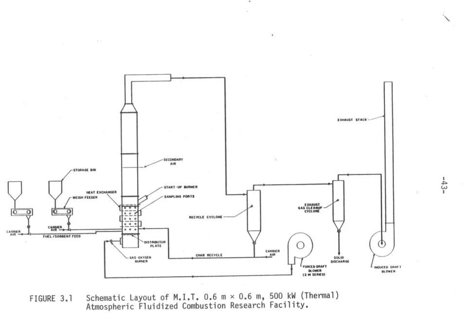
The atmospheric fluidized bed combustor which was used for these experiments was built and is operated by the Energy Laboratory at M.I.T. A schematic layout of the Fluidized Combustion Research Facility is shown

in Figure 3.1. The bed itself has a square cross-section which is 0.61 meters on a side and is 4.4 m tall. It has a nozzle type distributor plate with a square array of 64 nozzles. Each nozzle has four holes

(5.1 mm diameter) drilled radially, 7.5 cm from the base (see Figure 3.2).

in-STORAGE SIN

HEAT EXCHANGER

WEIGH FEEDER """""

CARRIER

AIIS

CA R IERFUEL /SORKEM FEED

GAS-OXYGEN BURNER SECA"f AR START-UP SI SAMPLG PC LATEI SITS RECYCLE CYCLONE -CHAR RECYCLE EXHAUST STACK--EXHAUST GAS CLEANUP CYCLONE SOI

FOMCD DRAIFT INOJ

SLOWER (aIN SERIES)

FIGURE 3.1 Schematic Layout of M.I.T. 0.6 m x 0.6 m, 500 kW (Thermal) Atmospheric Fluidized Combustion Research Facility.

IA

CEO DRAFT

U

-44-DISTRIBUTOR

PLAN VIEW

64 nozzles

15.88

(3.97

mm OD

)

E

L

4 -

5.08

mm

D

(1.27)

4

0.61 m (0.15)

FIGURE 3.2 Hot and Cold Bed Distributor Layout and Nozzle

Design (Cold Bed Dimensions are Shown in Parentheses.)

-45-jected into the side of the bed, near the distributor, through two in-dependent pneumatic feed systems. The heat of combustion is carried away from the bed by heat exchanger tubes which can either be immersed in the fluidized bed material and/or located in the freeboard. Each is made from 3.2 cm diameter tubing and has approximately 0.3 m2 of heat transfer sur-face area.

The bed becomes fluidized by the action of air which is forced up through the distributor nozzles from the plenum. The plenum is, in turn, pressurized by two forced draft fans placed in series on the inlet duct. In addition, the freeboard pressure can be controlled by an induced draft fan which is located on the exhaust side of the combustor. For a more detailed description of the combustor facility see reference [13].

Distributor air mass flow rate is measured by means of a pitot static tube located on the inlet side between the gas-oxygen burner and the forced draft blowers (not shown in figure). Carrier air, through the two fuel/sorbent feed lines, is measured upstream of the weigh feeders by separate rotometers. Typically, the portion of total fluidizing air that enters the bed through the two fuel lines, varies from 10% (when coal is burned and only one fuel line is used) to 50% (when oil shale is burned and both fuel lines are required).

For characterizing the performance of the furnace, there are provi-sions for inserting probes into the bed at some 70 locations. For instance, average pressure was measured at several different heights above the dis-tributor using water manometers which are connected to taps on the walls of the bed. This information is used, among other things, to determine the

-46-fluidized bed height in the combustor. Thermocouple probes are also located along a common vertical axis and were used to calculate the average bed temperature. (It should be mentioned that the temperature

rarely varied by more than 10C fromlocation to location.) At other locations on the walls of the combustor are special ports in which solid sampling probes may be inserted and through which samples of the bed material are drawn out during an experiment.

Figure 3.3 is anisometric view of the hot bed which shows the relative positions of some of the pertinent bed internals. The probes that are shown are those which were used to collect pressure fluctuation data or had a significant affect on the fluid mechanics of the bed. Among the intervals which are not shown are thermocouple probes, solid sampling probes and any probes which were in the freeboard (since they would have no effect on the fluid mechanics of the bed).

3.2 The Cold Bed

The scale model cold bed was built by Dalrymple [14] in the Mechanical Engineering Department to replicate the 0.61 m.xO.61 m. fluidized bed com-bustor. The cold bed is a geometric copy of the hot bed, with all dimen-sions scaled down by a factor of four (according to the scale factor from Table 2.1, (L.₁, L2' -- )cold be3 = 0.25 (LI, L2, L3 ''')hot ). The bed

bed' bed

is a square cross section column which is 0.15 m. on a side and 1.2 m. tall. One of the sides is made of clear plexiglass to allow visual observation of the fluidization. The distributor plate has plastic nozzles which are

geometrically similar to the steel nozzles in the hot bed and the nozzles dimensions were scaled by the same 4 to 1 ratio (the distorted length

-47-Dimensions Shown are Measured from Center Line of Distributor Nozzle Openings

FIGURE 3.3 Hot and Cold Bed Internal Configuration

(Cold Bed Dimensions are Shown in Parentheses.)

lyeo'

46'**

(9 0) 11k

,?less S*.

-,0 e

SO

eq

W

-48-scale discussed in Section 2.3 to compensate for thermal effects near the distributor was not used for these experiments). The nozzle pattern, the number of nozzles and the number of holes in each nozzle was of course

kept the same.

A schematic diagram of the entire cold bed laboratory apparatus is shown in Figure 3.4. The cold bed was designed to model the air flows in the hot bed which enter through the distributor nozzles and through the fuel/sorbent pneumatic feed lines. Air mass flowrates through the three branches (two feed lines and one line that supplies the plenum for the distributor air) are measured separately by square edge orifice flow-meters and the flows are controlled by needle valves.

Probe ports were drilled in the cold bed at locations which corres-pond to the positions of the probe ports in the hot bed. Water mano-meters were connected to taps along a common vertical axis of the column to measure average bed pressure. This data is used, as in the hot bed, to determine the fluidized bed height.

One aspect of the hot bed which was not modelled in the cold bed was the solid fuel flow through the feed lines. This was done to simplify the cold bed model. Its effects on the fluid mechanics in the cold bed will be discussed in Chapter 5.

Since all geometric aspects of the cold bed are identical, the isomet-ri~c view of the hot bed (Figure 3.3) can also serve as anisometric view for the cold bed. The cold bed dimensions are shown in parentheses next to the hot bed dimensions.

DUST FILTER

DUMMY

HEAT

EXCHANGER

TUBE

CARRIER AIR LINER

ORIFICE

FLOWMETERS

COMPRESSED

AIR

~-100

PSIG

SAMPL

PORT

ING

PRESSURE

REGULATORS

DISTRIBUTOR PLATE

ISTRIBUTOR AIR LINE

mT

H7~~

FIGURE 3.4 Schematic Layout of Cold Bed Laboratory Apparatus.

I