HAL Id: hal-02471456
https://hal.inria.fr/hal-02471456
Submitted on 8 Feb 2020
HAL is a multi-disciplinary open access
archive for the deposit and dissemination of
sci-entific research documents, whether they are
pub-lished or not. The documents may come from
teaching and research institutions in France or
abroad, or from public or private research centers.
L’archive ouverte pluridisciplinaire HAL, est
destinée au dépôt et à la diffusion de documents
scientifiques de niveau recherche, publiés ou non,
émanant des établissements d’enseignement et de
recherche français ou étrangers, des laboratoires
publics ou privés.
Toward real-time embedded observer of unsteady fluid
flow environment
Valentin Resseguier, Matheus Ladvig, Augustin Picard, Etienne Mémin,
Bertrand Chapron
To cite this version:
Valentin Resseguier, Matheus Ladvig, Augustin Picard, Etienne Mémin, Bertrand Chapron. Toward
real-time embedded observer of unsteady fluid flow environment. 10th European Congress on
Em-bedded Real Time Software and Systems (ERTS 2020), Jan 2020, Toulouse, France. �hal-02471456�
EMBEDDED REAL TIME SYSTEMS 2020 – Short paper
T
oward real-time embedded observer
of unsteady fluid flow environment
V. Resseguier
a, M. Ladvig
a, A. M. Picard
a,
E. Mémin
band B. Chapron
c[a] Lab, SCALIAN DS, Espace Nobel, 2 Allée de Becquerel, 35700 Rennes, FRANCE
[b] Fluminance team, Inria, Campus de Beaulieu, 263 Avenue Général Leclerc, 35042 Rennes, FRANCE [c] LOPS, Ifremer, 1625 Route de Sainte-Anne, 29280 Plouzané, FRANCE
Abstract:
For monitoring and actively controlling hydrodynamic and aerodynamic systems (e.g. aircraft wing), it can be necessary to estimate in real-time and predict the flow around those systems. We propose here a new method which combines data, physical models and measurements for this purpose. Very good numerical results have been obtained on 2- and 3-dimensional wake flows at moderate Reynolds, even 16 vortices shedding cycles after the learning window.
Keywords: state observer, data-driven, model-driven, low-order model, data assimilation
1. Introduction
Accurate aerodynamics active control (e.g. active flutter suppression) can require state observers. However, estimating in real-time -- or even predicting -- an unsteady turbulent flow state from sparse measurements is very challenging. To go beyond simple empirical estimation formulas, measurements can be coupled with flow dynamical models. Nevertheless, this path brings new difficulties.
First of all, such a dynamical system would need to resolve – in real time – enough spatio-temporal scales. On one hand, pure-data-driven fluid dynamics models (learned from e.g. least square, machine/deep learning) may not be accurate or robust enough. On the other hand, pure-physics-based model simulations (e.g. LES, RANS) are often too slow for real-time applications and can miss some important spatio-temporal scales. Reduced Order Models (ROM) are hence a good trade-off (see e.g. [9] for aeroelastic applications). In particular, the Proper Orthogonal Decomposition (POD) -Galerkin method relies on the physical equations while constraining the solution to live into a small subspace learned from data. Nevertheless, unsteady CFD ROM state of art is mainly limited to deterministic ROMs (often linear and/or with purely data-driven calibration) with weak prediction skills, especially because of the chaotic and intermittent nature of turbulence and of closure problems.
The simulation-measurement coupling, so-called data assimilation, is itself a challenging task. Thanks to the weather forecast community, there have been many advances from both research and operational perspectives. Notwithstanding, algorithms fully addressing non-linear dynamics – like fluid mechanics – are limited by the available computational effort and by the dynamical model accuracy quantification. We propose to overcome the first limitation with ROM. The second issue is the corner stone to combine the two distinct information sources which have different accuracies: numerical simulation outputs and measurements. This task is even more difficult for ROM [5]. We will here rely on the “dynamics under location uncertainty” -- a random fluid mechanics framework designed for this purpose [6,7].
Section 2 recalls the main aspects of POD-Galerkin ROM. Section 3 presents our main contribution: the randomized version of POD-Galerkin ROM. Section 4 explains the data assimilation procedure. Finally, section 5 presents our numerical results.
2. POD-ROM
Reduced order models (ROM) reduce computational costs of simulations by drastically reducing the solution degrees of freedom. This gain is enabled by the combination of simulation output data with physical models. In CFD, solutions
-- say the velocity field – have as many degrees of freedom as there are grid points over the spatial domain (say 105). In
ROM, velocity fields are traditionally decomposed as follows:
𝒗(𝒙, 𝒕) = 𝒗̅(𝒙)⏟ 𝐓𝐢𝐦𝐞 𝐚𝐯𝐞𝐫𝐚𝐠𝐞𝐝 + ∑ 𝒃𝒊(𝒕)𝝓𝒊(𝒙) 𝒏 𝒊=𝟏 ⏟ 𝐑𝐞𝐬𝐨𝐥𝐯𝐞𝐝 𝐛𝐲 𝐭𝐡𝐞 𝐑𝐎𝐌 + 𝒗′(𝒙, 𝒕) ⏟ 𝐕𝐞𝐥𝐨𝐜𝐢𝐭𝐲 𝐧𝐞𝐠𝐥𝐞𝐜𝐭𝐞𝐝 𝐛𝐲 𝐭𝐡𝐞 𝐑𝐎𝐌 , (𝟏)
with 𝑛 of the order of 10 or 102. Proper orthogonal decomposition (POD) learns the time averaged 𝑣̅(𝑥) and the spatial
modes 𝜙𝑖(𝑥) from a principal component analysis (PCA) applied to a set of high-resolution simulation outputs (learning period). Then, one can project the physical equations (e.g. Navier-Stokes equations) onto the spatial modes. This so-called POD-Galerkin algorithm provides a system of 𝑛 coupled ordinary differential equations describing the evolution of the temporal modes 𝑏𝑖(𝑡). Then, from time integration of this low-dimensional system and from equation (1), we can predict an approximation of the velocity field at a priori any time.This ROM construction stands halfway between fully data-driven methods and pure physical simulations. It takes advantage of the coupling between available data and physical models in order to infer reliable new prediction faster.
3. Model uncertainty quantification and data assimilation
Models under location uncertainty are a type of random CFD models [6,7]. It provides bothan efficient closure (i.e. an efficient way to model the effect of the neglected dynamics degrees of freedom 𝑣′) and an efficient quantification of the errors induced by this closure. In order to represent that uncertainty (inherent to any closure in CFD), multiple simulations are run in parallel using the random model and they efficiently cover the likely futures of a fluid system. Since that stochastic closure is based on physics, it is very robust, calibrations can be done from available physical quantities and almost no tuning nor fitting is needed.
Following the chapter 8 of [8], we have performed the POD-Galerkin of the Navier-Stokes model under location uncertainty. This procedure involves technical statistical estimations based on stochastic calculus. The interested reader can refer to [8] for more details. The ensuing low-dimensional system involves noises enabling model uncertainty quantification. Then, this random system can be used to make forecasts, even outside the learning period.
Sequentially in time, the random POD-ROM is coupled with measurements, using a particle filter with tempering and non-Gaussian mutation [2,3,1].
4. Numerical results
Our data assimilation procedure has been applied to 2- and 3-dimensional cylinder wake flows at Reynolds number 100 and 300 respectively. In these flows, vortices are shed from the cylinder in a pseudo-periodic way. Before our data assimilation tests, we have performed direct numerical simulations (DNS) using Incompact3d, a high-order flow solver, based on the discretization of the incompressible Navier-Stokes equations [4]. The simulation spatial grids correspond to state space dimension of about 104 at Reynolds 100 and about 106 at Reynolds 300. 100 and 80 vortex shedding
cycles are used for the ROM constructions (learning period) at Reynolds 100 and 300 respectively. The remaining vortex shedding cycles are used to test and to build synthetic measurements. For this first test, we assume that the resolved temporal modes 𝑏1(𝑡), … , 𝑏𝑛(𝑡) are directly observed, up to a strong additive noise. For every vortex shedding cycle, one of these measurements is assimilated by the random ROM. To model large measurement errors and/or measurements sparse in space, we choose a low signal to noise ratio (SNR=2dB) for the measurements.
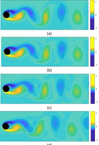
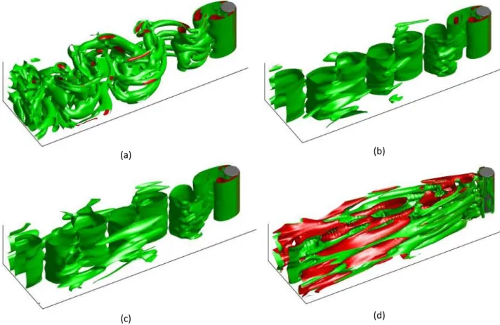
Despite the weak information contained in the measurements, the ROM shows very good prediction skills even outside the learning period, as illustrated by Figures 1 and 2. References are the DNS outputs, shown in Figures 1(a) and 2(a). The proposed observers (Figures 1(c) et 2(c)) are almost identical to the best possible estimations that could be obtained from 6-dimensional systems (Figures 1(b) et 2(b)). It illustrates the strong potential of our approach. Those optimums (Figures 1(b) et 2(b)) are theoretical performance limits: they correspond to the case of exactly known temporal modes 𝑏𝑖(𝑡) in the equation (1). The differences between those theoretical optimums (Figures 1(b) et 2(b)) and the DNS references (Figures 1(a) et 2(a)) is the unresolved velocity 𝑣′. At Reynolds 100, this difference is almost zero. At Reynolds 300, it is restricted to small scales and 3 dimensional effects. In order to better appreciate the strong skills of our observer, Figures 1(d) et 2(d) show predictions from benchmark deterministic POD-ROMs (POD-Galerkin with optimally fitted eddy viscosity) with the exact initial conditions but without data assimilation. At Reynolds 100, Figures 1(d) shows that this ROM predicts the vortices at wrong positions. At Reynolds 300, this benchmark ROM begins to diverge one vortex shedding cycle after the learning period.
To generate the simulation dataset, the off-line high-resolution CFD code runs during several hours on a supercomputer. The off-line ROM construction takes several hours on a laptop with a non-parallelized MATLAB® code. In contrast, the on-line ROM simulation -- assimilating measurement data on-the-fly – approximately runs in real (non-dimensional) time (i.e. one vortex shedding cycle every 5 seconds) also on a laptop, with a non-parallelized Python™ code. Huge speed-ups are expected with a C++ implementation for the off-line procedure, an embedded system for the on-line one and parallelization for both.
5. Conclusion
In this paper, we have proposed a new accurate and very fast method to estimate and predict a flow velocity field globally in space from sparse measurements. Comparisons with a benchmark approach have showed a huge improvement. Our algorithm is based on a random low-dimensional system built from physics and past DNS data, and the coupling of this system to measurements.
Currently, we generate synthetic particle image velocimetry (PIV) measurements. First assimilations results are very good. In the near future, we will assimilate real particle image velocimetry (PIV) measurements. Then, the methodology will be improved in order to address more turbulent flows and parametric ROMs. Eventually, thanks to the very low dimensionality of the random system, our method will be deployed in real-time embedded systems.
(a)
(b)
(c)
(d)
Figure 1: Vorticity fields (local spinwise velocity quantification) at Reynolds 100 -- 20 vortex shedding cycles after the learning period
a) Reference simulation (2D Direct Numerical Simulation (DNS): state space dimension of about 104)
b) The closest possible velocity field that can be obtained from the 𝑛-degree-of-freedom decomposition (1) (theoretical optimum for 𝑛 = 6)
c) Prediction from our POD-ROM-based data-assimilation (POD-ROM state space of dimension 𝑛 = 6)
d) Prediction from a benchmark deterministic POD-ROM (POD-Galerkin with fitted eddy viscosity) with the exact initial condition but without data assimilation (POD-ROM state space of dimension 𝑛 = 6)
(a) (b)
(c) (d)
Figure 2: Q-criterion fields (visual representation of vortices) at Reynolds 300-- 16 vortex shedding cycles after the learning period
a) Reference simulation (3D Direct Numerical Simulation (DNS): state space dimension of about 106)
b) The closest possible velocity field that can be obtained from the 𝑛-degree-of-freedom decomposition (1) (theoretical optimum for 𝑛 = 6)
c) Prediction from our POD-ROM-based data-assimilation (POD-ROM state space of dimension 𝑛 = 6)
d) Prediction from a benchmark deterministic POD-ROM (POD-Galerkin with fitted eddy viscosity) with the exact initial condition but without data assimilation (POD-ROM state space of dimension 𝑛 = 6)
References
[1] Cotter, C., Crisan, D., Holm, D. D., Pan, W., & Shevchenko, I. (2019). “Sequential Monte Carlo for Stochastic Advection by Lie Transport (SALT): A case study for the damped and forced incompressible 2D stochastic Euler equation”. In preparation. [2] Doucet, A., and Adam J. "A tutorial on particle filtering and smoothing: Fifteen years later." Handbook of nonlinear filtering
12.656-704 (2009): 3.
[3] Kantas, N., Beskos, A., and Jasra, A.. "Sequential Monte Carlo Methods for High-Dimensional Inverse Problems: A Case Study for the Navier--Stokes Equations." SIAM/ASA Journal on Uncertainty Quantification 2.1 (2014): 464-489.
[4] Laizet, S., and Lamballais., E. "High-order compact schemes for incompressible flows: A simple and efficient method with quasi-spectral accuracy." Journal of Computational Physics 228.16 (2009): 5989-6015.
[5] Livne, E. "Aircraft active flutter suppression: State of the art and technology maturation needs." Journal of Aircraft 55.1 (2017): 410-452.
[6] Mémin, E.. "Fluid flow dynamics under location uncertainty." Geophysical & Astrophysical Fluid Dynamics 108.2 (2014): 119-146.
[7] Resseguier, V., Mémin, E., and Chapron, B.. "Geophysical flows under location uncertainty, Part II Quasi-geostrophy and efficient ensemble spreading." Geophysical & Astrophysical Fluid Dynamics 111.3 (2017): 177-208.
[8] Resseguier, V.. Mixing and fluid dynamics under location uncertainty. Diss. Université Rennes 1, (2017).
[9] Thomas, P., Earl D., and Kenneth H.. "Three-dimensional transonic aeroelasticity using proper orthogonal decomposition-based reduced-order models." Journal of Aircraft 40.3 (2003): 544-551.