Parameter Free Image Artifacts Detection: A Compression Based Approach

HAL Id: hal-00687318

https://hal.archives-ouvertes.fr/hal-00687318

HAL is a multi-disciplinary open access

archive for the deposit and dissemination of

sci-L’archive ouverte pluridisciplinaire HAL, est destinée au dépôt et à la diffusion de documents

Parameter Free Image Artifacts Detection: A

Compression Based Approach

Avid Roman Gonzalez, Mihai Datcu

To cite this version:

Avid Roman Gonzalez, Mihai Datcu. Parameter Free Image Artifacts Detection: A Compression Based Approach. SPIE Remote Sensing, Sep 2010, Toulouse, France. pp.783008. �hal-00687318�

Parameter Free Image Artifacts Detection: A Compression Based

Approach

Avid Roman-Gonzalez

, Mihai Datcu

_{TELECOM ParisTech, 75013 Paris, France}

_{German Aerospace Center (DLR), Oberpfaffenhofen}

ABSTRACT

The qualified Earth Observation (EO) images sometimes may present unexpected artifacts. These perturbations and distortions can make more difficult the analysis of images and may decrease the efficiency of interpretation algorithms because the information is distorted. Thus is necessary to implement methods able to detect these artifacts regardless of the model which are formed, i.e. parameter free. In this article, we propose and present a method based on data compression, whether lossy compression or lossless compression for detecting aliasing, strips, saturation, etc.

1. INTRODUCTION

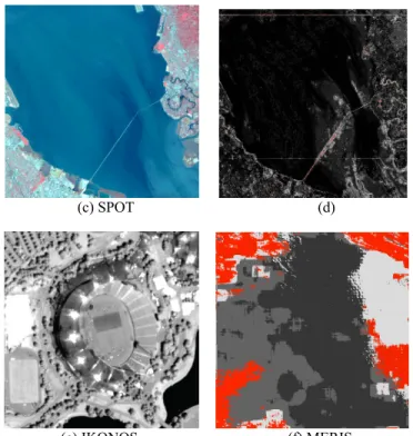
The qualified EO images, sometimes may present unexpected artifacts, distortions or artificial structures which can be produced by the instrument itself or due to pre-processing. These perturbations may come from miss adaptation of the sensor resolution for the scene detected, thus aliasing may occur, artifacts due to eventual compression of the EO product, potential saturation of the sensor for particular image geometry, accidental image stripes or bands, etc. These perturbations and distortions can make more difficult the analysis of images and may decrease the efficiency of interpretation algorithms because the information is distorted. The artifacts produce very small variations in gray level. The growing volume of data provided by different sources of images requires the use of tools to perform analysis automatically, such as similarity detection, classification, pattern recognition, etc. Fig 1 shows some examples of artifacts, in (a) and (b) we can see a change of texture; (c) and (d) show the existence of horizontal lines which can be detected as bridges; (e) shows the saturation and (f) shows the blocking. All these processes may be affected if the image has artifacts, these artifacts may interfere with the recognition of a texture or the quantification of features. The nature of some of these artifacts is unknown and varied, these artifacts doesn’t have the same models, that is why it is necessary to implement methods able to detect these artifacts regardless of the model which are formed, i.e. parameter free.

In the process of elaborating the standard product of a satellite image, there is a process of correction of artifacts as presented by Hyung-Sup in [1] which is an algorithm for the restoration of defectives lines; however some artifacts may be remaining after this process.

(a) (b)

(c) SPOT (d)

(e) IKONOS (f) MERIS

Fig. 1 Some Examples of Artifacts: (a) and (b) Shows a change of texture by aliasing. (c) Shows a sea picture where there a bridge. (d) Shows the existence of horizontal lines and these lines could be detected as bridges by an algorithm for indexing. (e) Shows saturation

of the sensor. (f) Shows the blocking in the picture.

The work presented in this paper is the continuation of the work by A. Mallet in [2] and [3]. In this article, we propose the use of compression techniques, lossless and lossy compression, such as parameter-free method for the artifacts detection like aliasing, strips, saturation, etc. Using these compression techniques the aim is to evaluate the level of regularity or irregularity that may have an artifact.

In this article we propose two methods: The first method uses Lossy Compression to calculate the Rate-Distortion Function. The Rate-Distortion analysis allows us to evaluate how much the data was distorted, we further develop and asses the method in [3] based on the analysis of the lossy compression error for variable compression factor. The error behavior of the sectors with artifacts is different from the sectors that do not contain artifacts. Second method uses the Lossless Compression to calculate Normalized Compression Distance (NCD), the NCD is a method proposed by M- Li in [4] to determine the similarity between two files using a distance measure based on Kolmogorov complexity. The paper is structured as follow. Section II presents an overview on the theory on which these methods are based. Section III shows practical applications in artifacts detection in optical images. Finally section IV reports our conclusions.

2. THEORETICAL BACKGROUND

2.1 Rate – Distortion Function

The Rate-Distortion (RD) Function is given by the minimum value of mutual information between source and receiver under some distortion restrictions.

Where:

)

,

( Q

p

I

The RD function shows the compression error given for different compression factor.

The RD function depends of the visual complexity, for example plotting Experimental RD Curve, we can do an analysis of the image, for example Fig. 2 shows two images in (a) shows an image that has a lot of detail because it contains hills, houses, trees, cars, people, etc; while in (b) we have a picture without much detail that the background appears to be constant and the color of the dogs too. This analysis is reflected in the experimental RD curve shown in Fig. 3 in which we can see that the curve of the image (a) which is the blue line is above to the curve of the image (b) which is the green. Can be considered that the artifacts increase the complexity in the image, for example we can do the same experiment to see the change in the experimental RD curve of any image and the same image but with synthetic lines added, in Fig. 4 (a) shows the normal Cusco city image and Fig. 4 (b) shows the Cusco city image but with some defectives lines. We can observe in Fig. 5 the experimental RD curves for each image, blue for (a) and green for (b), we can see that the curve of the image with defectives lines is above to the curve of the normal image, this is because the defects cause that the image is more irregular. To calculate RD Function, is used Baseline-JPEG as a lossy compressor.

(a) Cusco City (b) Puppies

Fig. 2: (a) Cusco City is an image with a lot of detail; it contains hills, houses, trees, cars, people, etc. (b) Puppies is an image with a background almost constant, this image is less complex than image (a).

0 10 20 30 40 50 60 70 80 90 100 0 20 40 60 80 100 120 140 160 180

Fig. 3 Experimental Rate-Distortion Curve: blue for Fig. 2 (a) and green for Fig. 2 (b), the experimental RD curve for the complex image (a) is above than the experimental RD curve for image (b).

)

,

(

min

)

(

D

I

p

Q

R

=

(a) Cusco City (b) Cusco City with Defectives Lines

Fig. 4: (a) Cusco City is an image normal. (b) Is the same image (a) but with defectives lines artificially introduced to analyze its influence to the calculation of experimental RD curve.

0 10 20 30 40 50 60 70 80 90 100 0 50 100 150 200 250 300 350

Fig. 5 Experimental Rate-Distortion Curve: blue for Fig. 4 (a) and green for Fig. 4 (b), the experimental RD curve of normal image is below than the experimental RD curve of image with defectives lines

2.2 Normalized Compression Distance (NCD)

The Kolmogorov Complexity K(x) of an object x is the minimum amount of computational resources (q) needed to represent x. The Kolmogorov Complexity is defined by:

( )

min

K x

q

=

Q

There is a dependency of the size and descriptive language, but it is not very worrying as it is reduced to some constant, i.e., given two languages L1 and L2, and any string of symbols x, |K1(x)-K2(x)| < k. For move from a description in L1 to

another in L2 is a program interpreter of L1 in L2 writing. The interpreter may be more or less long, but it's fixed, so that

its size is a constant.

Within the Information Theory we can say that the Kolmogorov complexity or algorithmic complexity is the amount of information needed to recover x. It is important to note that K(x) is a non-calculable function. The conditional complexity

K(x, y) of x related to y is defined as the length of the shortest program with which we can obtain an output x from y. An

important application of this notion is to estimate the shared information between two objects: The Normalized

Information Distance (NID) [1]. The NID is proportional to the length of the shortest program that can calculate x given y. The distance calculated from these considerations is then normalized as follows:

(a) (b)

(1)

( )

( )

{

( ) ( )

}

( ) ( )

{

}

The NID result is a positive value r in the range of: 0 ≤ r ≤ 1, with r = 0 if the objects are identical and r = 1 is the maximum distance between them.

The compressibility is a term that derives from having a small program P that describes a string x. Therefore, if K(x) <

|x| we say that x is compressible.

The Normalized Compression Distance NCD has a definition as follows: Since the Kolmogorov Complexity K(x) is a non-computable function, an approximation is defined by Li in [1] considering K(x) as the compressed version of x, and a lower limit of what can be achieved with the compressor C.

Previous research [1, 2] use the Kolmogorov Complexity for define the Normalized information Distance NID and from there derive the Normalized Compression Distance. It is to approximate K(x) with C(x) = K(x) + k, the length of the compressed version of x obtained by a lossless compressor C plus an unknown constant k: the presence of k is necessary because it is not possible to estimate how close of K(x) is this approach.To clarify this concept, we take two strings b y p have the same length n, where the first is a random output of a Bernoulli process and the second represents the first n digits of π. The quantity K(p) would be smaller tan K(b) because there is a program of length K(p) << n which output is the number π, while a program that has as output a random sequence of bits would have a close to n length, is so K(p) <<

K(b).Thus, the equation (1) could be estimated by the Normalized Compression Distance (NCD) as shown in equation (2): (2)

(

)

(

)

{

( ) ( )

}

( ) ( )

{

}

C(x, y) represents the size of compressed file obtained by the concatenation of x and y.

The NCD can be calculated explicitly between two strings or two files x and y, and this represents how different are these files, facilitating the use of this result into various applications with different data into a parameter-free approach [2, 5] and classify them by unsupervised methods [6]. The NCD is a positive result 0 ≤ NCD ≤ 1+e, with e as a representation of imperfections of the compression algorithms. It is necessary to remark that the K(x) approximation with C(x) depends on the data with which to work, knowing that common compressors are built base don different hypotheses, some are more efficient than others with a specific type of data. In this article we using a JPEG-LS compressor because the JPEG is a compressor oriented to images, then its performance is higher compared to a general purpose compressor [7].

3. EXPERIMENTS AND RESULTS

3.1 Artifacts Detection Using Rate – Distortion Analysis

For the artifacts detection, we propose to use the RD function obtained by compression of the image with different compression factors and examine how an artifact can have a high degree of regularity or irregularity for compression. The RD Analysis is done as the blocks diagram shown in Fig. 6, first we take the image under test, we compress the image with different compression factors, then decompress the image and calculate the error for each compression factor, based on the errors we make a features vector and then apply classification methods.

Fig. 6 Block Diagram for Rate-Distortion Analysis: we take the image under test, we compress the image with different compression factors, then decompress the image and calculate the error for each compression factor, based on the errors we make a features vector

and then apply classification methods

A) Case Study 1 – Validation with Synthetic Data:For doing this experiment, we use artificial artifacts in images, so we

have simulated the aliasing artifact. For simulating aliasing in an image, is necessary a downsampling process of the image, while we do the downsampling, aliasing occurs and to avoid aliasing, is necessary a low pass filter before downsampling process; taking these considerations, the simulation of aliasing used for this experiment was do following scheme of Fig. 7.

Fig. 7 Aliasing Process Simulation, first we make a downsampling process of the image, while we do the downsampling, aliasing occurs and to avoid aliasing, is necessary a low pass filter before downsampling process

After applying the methodology presented to the image with aliasing, the results for the aliasing detection is shown in Fig. 8, where we can clearly see the areas that contain the aliasing.

(a) Image with Aliasing (b) Aliasing Detection

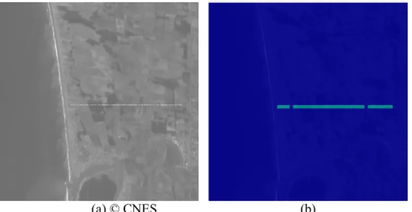
B) Case Study 2 – Validation with Actual Data:Another result of artifacts with RD, it is the Dropout detection shown in

Fig. 9, In this case it is a SPOT image containing actual artifacts, the detection is done correctly.

(a) © CNES (b)

Fig. 9 Dropout (SPOT). (a) Some electronic losses during the image formation process create these randomly saturated pixels. The dropouts often follow a line pattern (corresponding to the structure of the SPOT sensor). (b) Artifact is detected.

3.2 Artifacts Detection Using Normalized Compression Distance (NCD)

For this methodology, we take the satellite image and divide it into patches of 64x64 pixels, with these patches we calculate the distance matrix between them using NCD and finally we applied a hierarchical classification method to cluster and identify the patches with artifacts. This process can be seen in Fig. 10.

Fig. 10 Experiment Process: we take the satellite image and divide it into patches of 64x64 pixels, with these patches we calculate the distance matrix between them using NCD and finally we applied a hierarchical classification method to cluster and identify the

patches with artifacts

In this part we will use two datasets, a dataset of satellite images with artificial artifacts introduced manually; and another dataset of satellite images with real artifacts introduced by the sensor itself.

A) Case Study 1 – Validation with Synthetic Data: For the images with artificial artifacts, we introduce two types of

artifacts with different intensities in such a way to study their behavior; these artifacts introduced manually can be seen in Fig. 11, in the first instance we introduce strips with different levels of intensity, which is done is to increase the grayscale value of the satellite image in the desired positions. For the aliasing simulation, we also use different values of down sampling. The introduction of artificial artifacts is made with different intensities to assess the sensitivity of the detection method.

Fig. 11 Artifacts Simulation with Various Intensities: the first artifacts are the strips with different levels of intensity, which is done is to increase the grayscale value of the satellite image in the desired positions. The second artifact is aliasing simulation; we also use

different values of down sampling.

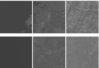
Then, we have a database with different types of artifacts with different intensities and in different environments such as: city, forest and sea; as shown in the following images:

Fig. 12 Satellite image database for our experiment with different types of artifacts such as strips and aliasing, with different intensities and in different environments such as city, forest and sea.

After making de division of the image into patches of 64x64 pixels as explained in the procedure as shown in Fig. 13, we apply a hierarchical classification method whose results are shown in Fig. 14. The Dendrogram is a type of graphical representation of data as a tree that organizes the data into subcategories that are dividing in others to reach the level of detail desired, this type of representation allows appreciating clearly the relationship between data classes. To plot the dendrogram we use the Euclidean Distance method.

Fig. 13 Separate image in patches of 64x64 pixels for calculate the distance matrix between the patches

To evaluate the proposed method, we made a study of detection sensitivity with different levels of intensity of the artifact, so also this study has been done in different environments such as: sea, forest and city. So our database contains images of different environments with different types of artifacts at different levels of intensity.

Fig. 14 Hierarchical Classification of the Patches: we can see two cluster, red cluster for patches with artifacts, and cyan cluster for patches without artifacts.

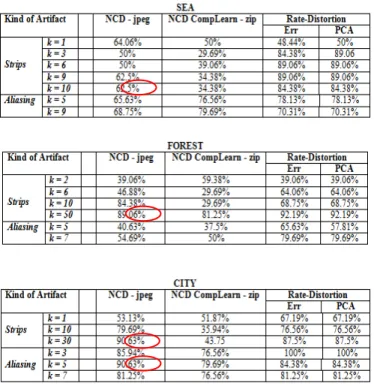
Finally, after applying the method to our database, the results expressed as percentage of success are:

In the table above, we can see the results for the different environment: sea, forest and city, with the strips and the aliasing artifacts in different intensities. The NCD calculation was made using different compressors as JPEG and zip. The intensity of the strips for detection is lower in the sea. The better detection of aliasing occurs in the city because the bandwidth is wider.

B) Case Study 2 – Validation with Actual Data: For images with real artifacts, we take images acquired by the ROSIS

sensor provided by the German Aerospace Center (DLR); these data are hyperspectral images of 7946x512 pixels, 16 bits and 115 bands. We work with subscene of 512x512 pixels as the example in Fig. 15. First thing, we make a manual analysis to determine the location of artifacts, thus we detect strips in the last two bits as shown in Fig. 16.

Fig. 15 Examples of 512x512 subscenes with real artifacts, the image is acquired by ROSIS sensor provided by German Aerospace Center (DLR).

Fig. 16 Bit by Bit Analysis for Strips Detection in the ROSIS Image: we can see the strips in the last bits. After applying the proposed method, the results are not encouraging and are shown in the following table:

These bad results may be because the strips are presented in the last bits are indexed not detected.

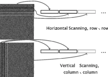
Given these results, the next experiment is to take directly the binary image containing strips, divided it into 64x64 patches as shown in Fig. 17 and each patches convert to a text string with values of 0s and 1s, then calculate the Normalized Compression Distance with these strings and finally apply the hierarchical classification. For make the conversion to text string, we have two possibilities, a horizontal scanning or vertical scanning as shown in Fig. 18. As each patch has 64x64 pixels and to form the text string we order either row or column after another, then finally each text string will be formed by 4096 values.

Fig. 18 Formation of the text string based on binary images: we have two options for scanning process, horizontal scanning and vertical scanning. We form the text string order either row or column after another, then finally each text string will be formed by

4096 values

The results after to apply the proposed approach is shown in the following table:

Horizontal Scanning Vertical Scanning

NCD for text Total mixture 81.25%

The results for vertical scanning are much better because the strips have the same vertical orientation.

Finally we have developed a small tool to do an artifact detection process using the previously methods reported, the interface tool is shown in Fig. 19. This interface has the methods proposed, both, the calculation of NCD as also the use of Rate-Distortion function; in this interface it is possible to vary the size of patches.

Fig. 19 Tool for Artifacts Detection: With this interface we can apply the different methods proposed, both, the calculation of NCD as also use the Rate-Distortion analysis; in this interface it is possible to vary the size of patches

4. CONCLUSIONS

The conclusions are in function of two datasets: About the artificial artifacts

ƒ We can appreciate that the strips have an acceptable possibility to be detected in a sea environment from an intensity of k = 10, however in the forest and the city environment with intensity k = 30.

ƒ The aliasing can be detected in a city environment, but not at sea or in the forest, due to de city’s bandwidth is widest than the sea and forest.

ƒ The detection of artifacts is done best way depending on the environment we are working, at sea and in the field is easier to detect the strips but not so the aliasing, while in the city and the forest is easier to detect aliasing. About the real artifacts

ƒ We can see that there aren’t good results and this may be because the strips are presented in the last bits and can not be detected.

ƒ The acceptable results are found with scanning vertically, column by column as the strips also have the same orientation.

5. ACKNOWLEDGMENT

HyMap was made available from HyVista Corp. and DLRs Optical Airborne Remote Sensing and Calibration Facility service (http://www.OpAiRS.aero), and the ROSIS data by DLRs OpAIRS service (http://www.OpAiRS.aero). The authors very much acknowledge the support of Dr. Martin Bachmann from DLR.

REFERENCES

[1] J. Hyung-Sup, W. Joong-Sun, K. Myung-Ho, L. Yong-Woong, “Detection and Restoration of Defective Lines in the SPOT 4 SWIR Band”, IEEE Transaction on Image Processing, 2010.

[2] D. Cerra, A. Mallet, L. Gueguen, M. Datcu, “Algorithmic Information Theory Based Analysis of Earth Observation Images: an Assessment”, IEEE Geosciences and remote Sensing Letters, in press.

[3] A. Mallet, M. Datcu, “Rate Distortion Based Detection of Artifacts in Earth Observation Images”, IEEE

Geosciences and Remote Sensing Letters, vol. 5, N° 3, pp. 354-358, July 2008.

[4] M. Li, X. Chen, X. Li, B. Ma, P. M. B. Vitanyi; “The Similarity Metric”, IEEE Trans. Inf. Theory, vol. 50, N° 12, pp. 3250-3264.

[5] E. Keogh, S. Lonardi, Ch. Ratanamahatana, “Towards Parameter-Free Data Mining”, Department of Computer

Science and Engineering, University of California, Riverside.

[6] R. Cilibrasi, P. M. B. Vitanyi; “Clustering by Compression”, IEEE Transaction on Information Theory, vol. 51, N° 4, April 2005, pp 1523 - 1545.

[7] T. Tao, A. Mukherjee, and R.V. Satya, “A search-aware JPEG-LS variation for compressed image retrieval”,