MODEL OF HIGH-SPEED TRAIN ENERGY CONSUMPTION P-O. VANDANJON1, R. BOSQUET2, A. COIRET1 and M. GAUTIER3
1Université Bretagne-Loire, Ifsttar,
AME, EASE, Ifsttar, Route de Bouaye,
F-44341 Bouguenais, France
2SNCF-Direction du
matériel/Ingéniérie du matériel-Centre d'ingéniérie du matériel –
F-72100 Le Mans France
3Université de Nantes, IRCCyN
1, rue de la Noë BP 92 101, F-44321 Nantes
France
Received: November 7, 2016
ABSTRACT
The current transport system is not sustainable because of its high consumption of finite resources (mainly oil) and its impact on the environment (air quality, global warming, etc.). In this context, rail has several advantages: lower consumption and emissions than road and air modes, larger passenger flow, etc. That is why, many rail infrastructures are planned in the world. Today, the impact of energy is not taken into account during the project design. At the project phase of new rail infrastructures, it is nowadays important to characterize accurately the energy that will be induced by its operation phase, in addition to other more classical criteria as construction costs and travel time. Current literature consumption models used to estimate railways operation phase are obsolete or not enough accurate for taking into account the newest train or railways technologies. In this paper, an updated model of consumption for high-speed is proposed, based on experimental data obtained from full-scale tests performed on a new high-speed line. The assessment of the model is achieved by identifying train parameters and measured power consumptions for more than one hundred train routes. Perspectives are then discussed to use this updated model for accurately assess the energy impact of future railway infrastructures.
Keywords: identification, consumption model, high-speed line, high-speed train
1. INTRODUCTION
According to the International Transport Forum at the OECD [1]: Greenhouse gases emissions (GHG) due to the transport sector will increase by 34 % to 106 % between 2010 and 2050 depending on different economic scenarios. In the same time, the experts of the intergovernmental panel on climate change recommend to stabilize these GHG emissions from the transport sector in order to follow the representative concentration pathway 2.6 (RCP 2.6) to keep the global warming below 2° [2]. These two studies imply that our actual transport system is not sustainable.
One solution, among others, is to switch from the petrol to the electricity as energy source for the transport system. It will be very advantageous for countries where the electricity mix has a low carbon content as in France (due to the nuclear power) or in Norway (due to the hydraulic power).
In this context, high speed trains offer many advantages, as consuming significantly less energy than road or air transports. According to Akerman [3], high-speed transport consuming roughly 4 times less energy use than road transport and 9 times less than air transport (expressed as kilowatt-hour by passenger-kilometer - kWh/pkm). Even if Chester and Horvath [4] moderates this result with the life cycle assessment point of view, rail modes have the smallest energy consumption. So, about 10,000 km of tracks are under construction in the world and more than 15,000 km are planned as determined by UIC [5].
At a railway project, several alternative routes are usually studied. The final choice of the rail line is the output of a complex process including numerous actors as described by
Leheis [6]. The different stakeholders (national government, local authorities, local residents, economic sector, ecological associations, etc.) request objective methods in order to enlighten public debates. Our contribution is to propose a consumption model for high speed train in order to simulate different scenarios. Our first result was described in [7]. In this actual paper, an updated model is proposed which is a major improvement in comparison with this first paper by modelling the power for the mechanical and electrical part of the system. Moreover, the identification process is based on a robotic technique called IDIM-LS, more robust than the technique used in the first paper. This new approach yields to a more consistent and more accurate comprehensive model.
The next section builds the consumption model. This model depends linearly on parameters which are identified in the section 3 through experimental data. The last section concludes this paper.
2. COMPREHENSIVE MODEL
In this topic, the first approach is to reduce the train to a point and to apply the Newton's second law to this point. Lukaszewicz [8] or Rochard and Schmid [9] give an interesting general formulation of running resistance as a function of train characteristics like mass, number of bogies, inter-vehicle gap, number of pantographs, etc. Unfortunately in those models, the maximum speed is generally lower than 300 km/h although the projects speed of a new high-speed line are at least 350 km/h. Formulation presented in the current paper is an adaptation of these literature models to higher speeds by taking into account test data. Particularly, for high speeds, aerodynamic have to be analysed more accurately. Raghunathan et al. [10] study it for Shinkansen and their approach is adapted to the TGV Dasye in this paper.
Then, the second step of the model review is to gather knowledge on the method to convert the force developed by the train (based on a physical model) in energy consumption. Lindgreen and Sorenson [11] and Boullanger [12] propose a consumption model with information about engine efficiency, loss of auxiliary equipment and transformer. These models will not directly be used in this paper since they are not suitable for the electric French case (25 kV 50 Hz AC) and high-speed train.
Our comprehensive model is the union of a mechanical model and an electrical model. They are described in the following paragraphs.
2.1 The Mechanical Model
The mechanical model, described by figure 1, associated with the theorem the derivative of the mechanical energy is equal to the power of the non-conservative forces yield to the following equation :
(1)
Fm is the tractive force produced by the driving chain including the motor at the drive
wheels; V is the speed of the train; m is the mass; k is the conventional coefficient, it represents inertia of rotating masses; α is the slope of the rail line;
Frr is the running resistance and is composed of the following physical effects.
• Rolling resistance: it is related to the contact wheel rail. As a first approximation, it is considered as constant. Because of sticking effect, this value is not the same when the train is stop or sets in motion.
• Mechanical resistance: it consists of friction which are viscous friction Fc,
depending mainly of the velocity, and the dry friction Fs , which can be considered
as constant (unless when the train starts for the same reason as for the rolling resistance).
• Aerodynamic resistance, related to drag coefficient Cx , and the weather conditions
(wind, rain, etc...). This resistance depends mainly on the squared velocity.
By taking into account the previous physical interpretation, this resistance force (Frr) is
approximated by a second order polynomial [9]:
(2)
ρ is the air density; Vwind is the speed of the wind along the direction of the speed of
the train; A, B, C are coefficients depending on the rolling stock.
One speciality of our model is to multiply only A by the mass m. In [9], all the right side of the equation (2) is multiplied by the mass m. Our model is an adaptation of the classical models to High-Speed train for which the C term plays a major role and is not substantially influenced by the mass.
In our model, the resistance force in curve is not modelled. Knowing that the radius of high speed line is superior to 3,000m, and considering the model of this force given in [9], this resistance force can be neglected in a first approach.
2.2 Electrical model
Fig. 2 displays the electrical model and the different losses at each step of the transformation of the electrical power to the mechanical power. It is based on classical results in Electrical Engineering.
The input of this scheme is Pp the active power exchanged at the catenary with the
pantograph. Pp =Up Ip cos(Ф). Up Ip is the rms voltage and current delivered by the
pantograph. Ф is the current-voltage phase shift. Pp is positive while the engine is
providing traction and is negative while energy-recovery braking system is used. The output of this scheme is the power computed with the tractive force Pm = Fm V.
The first step is done by the transformer which decreases the initial voltage: 25 kV to 1kV, the copper losses are Pct =Rt Ip2. As the voltage is assumed constant, the iron
losses Pft are constant.
One part of the power after the transformer Pa, is consumed by the auxiliary equipment,
they are the cooling of the motor, the air-conditioning system, the lighting. As the tests were carried out in summer during the day, this loss is assumed to be constant.
The rectifier transforms alternative current (AC) to direct current (DC). The losses of the rectifier are proportional to Is, the secondary current output of the transformer.
Pro =du Is.
The motor of the train is asynchronous. The power loss is approximated by the following equation.
Pfm, Km1, Km2 are constant in relation with the iron losses in the stator; Im is the current
in the stator, Rm is an equivalent resistor.
The following equation is calculated by rearranging the previous equations and replacing the currents by the current delivered by the pantograph,
( 3)
PF, Km1 and Km2 are constant in relation with the iron losses; Du is a constant in
relation with the losses in the rectifier; R models the copper losses.
2.3 Comprehensive model
Finally, by combining equations 3 and 1 and regrouping parameters, the final equation of the power is
(4)
Pco, Du, R, A, B, C, m, k are parameters of the train (Pco regroups the constant terms).
V, Ip is the state of the system; ρ, Vwind are the meteorological conditions, α is the local
slop of the train line.
3. IDENTIFICATION
In the previous equation, some parameters are known thanks to public technical data: the mass of the train, m = 380 tons + estimated weight of the passengers, the model of the rotating inertia, k = 1.04, but most of them are unknown: Pco , Du , R, A, B, C. In
order to identify them, data of the acceptance tests of the High-Speed Line Rhin-Rhône were processed. It is the purpose of this section.
4. EXPERIMENT
The acceptance tests of the French Rhin-Rhône high- speed line have been used to obtain experimental data. The line has been opened to the traffic since the end of 2011 and links Mulhouse to Dijon, via Belfort-Montbéliard and Besançon
Numerous tests have been performed on this high-speed line. Among these tests, 130 trial runs (half in the east/west direction, half in the west/east direction) (79 hours of travels) have been carried out for the purpose of this study within a period of three months between June and August 2011. For field testing, 20 sensors were added to the test train. During these tests, geometry, energy, dynamic measurements, direction and velocity of the wind were recorded. A special attention was dedicated to the aerodynamic drag [13]. The test train is the standard French TGV Duplex DASYE (duplex asynchronous ERTMS). Speed, position and active power measured at the pantograph have been recorded at a 5 Hz.
5. RESULTS
A first analysis of the comprehensive model (equation 4) is that the equation is linear in relation to parameters. Then, this equation is rearranging to:
W is the observation matrix :
χbs is the vector of the basic parameters:
A well-known identification technique is to use linear least-squares which solve the
optimization program where ym is computed from the
measurements. However, the observation matrix is also built with measurements. In this case, the least-squares estimate does not converge to the true value. It is the reason why, a method coming form Robotic: IDIM-LS (Identification Dynamic Inverse Model – Least-Squares) was used (see [14]). It consists, mainly, to apply a filter on each signal and a parallel filter on each column of the observation matrix.
The identification process warns us that two parameters are not identifiable with the given experimental data: A and R. Finally, the following table presents the value of the essential parameters, their standard deviations, their units and the ratio between standard deviation and the value of the parameter.
Essential parameters sd( ) SI sd( )/ B 154 4 kg/s 2 % C 5.04 0.04 Kg/m 0.8 % Pco 287×103 5.3×10³ W 2 % Du 425×101 1.4×101 V 0.3 %
The parameters are well identified, the ratio sd( )/ is small. Moreover, we checked the physical meaning of the values by comparing them with fragmented technical data.
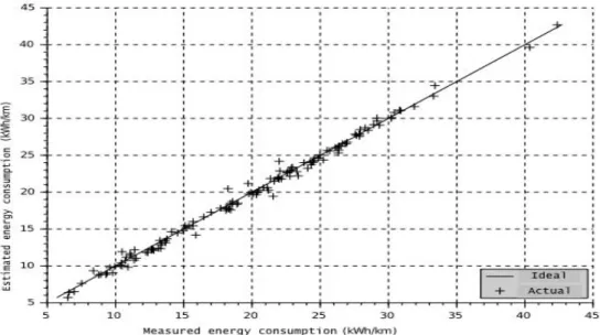
Fig. 3 Validation of the model
Fig. 3 displays a comparison between the measured and estimated energy consumption of the 130 trial runs. 95 % of the energy spent during the tests is explained by our model.
6. CONCLUSION
Numerous high-speed line projects arise due to the energy efficiency of this system of transport. However, it is important to assess in advance the impact of future energy lines. Unfortunately, there was no bibliography for consumption model which can be used to assess different routes from an energy point of view. In this paper, an energy consumption model is proposed to assess operation phase. Along a route, the model provides instantaneous power supply as well for acceleration, deceleration and constant speed phases in function of route profile. Thanks to this model, key infrastructure parameters affecting the energy consumption can be identified (see [15]). The energy consumption of the new 15,000 km of high-speed line, which are planned in the world, represents the issue of such energy models. This study is part of a global methodology called PEAM (Project Energy Assessment Method) which takes into account too the consumption of construction phase. This methodology was applied on the project of the High Speed Line Montpellier-Perpignan [16]. An unintended outcome of this study is a contribution to the eco-driving of train [17].
7. ACKNOWLEDGMENT
This investigation is part of a partnership with SNCF Réseau, the French railway owner. Tests were performed by SYSTRA (http://www.systra.com), EURAILTEST (http://www.eurailtest.com) and SNCF/AEF.
8. REFERENCES
[1] ITF Transport Outlook 2015. OECD Publishing, 2015.
[2] Pachauri, R.K. - Meyers,L.A.: Climate Change 2014: Synthesis Report. Contribu-tion of Working Groups I, II and III to the Fifth Assessment Report of the Intergovernmental Panel on Climate Change, IPCC. Geneva, Switzerland, 2014. [3] Akerman, J.: The role of high-speed rail in mitigating climate change − The
Swedish case Europabanan from a life cycle perspective, Transp. Res. Part
Transp. Environ., vol. 16, no 3, 2011, p.208-217.
[4] Chester, M. V. - Horvath, A.: Environmental assessment of passenger transport-ation should include infrastructure and supply chains, Environ. Res. Lett., vol. 4, no 2, avr. 2009, p.024008.
[5] High Speed - International Union of Railways (UIC). [En ligne]. Disponible sur: http://www.uic.org/highspeed. [Consulté le: 03-nov-2016].
[6] Leheis, S.: High-speed train planning in France: Lessons from the Mediterranean TGV-line, Transp. Policy, vol. 21, no 0, 2012, p.37-44
[7] Bosquet, R. - Vandanjon, P.-O. - Coiret, A. - Lorino, T.: Model of High-Speed Train Energy Consumption, in World Academy of Science, Engineering and Technology, 2013, vol. 78.
[8] Lukaszewicz, P.: Running resistance - results and analysis of full-scale tests with passenger and freight trains in Sweden, Proc. Inst. Mech. Eng. Part F J. Rail Rapid Transit, vol. 221, January, 2007, p.183-192.
[9] Rochard, B. - Schmid, F.: A review of methods to measure and calculate train resistances, Proc. Inst. Mech. Eng. Part F J. Rail Rapid Transit, vol. 214, no 4, 2000, p.185–199. [10] Raghunathan, R. S. - Kim, H.-D. - Setoguchi, T.: Aerodynamics of high-speed
railway train », Prog. Aerosp. Sci., vol. 38, no 6–7, 2002, p.469-514.
[11] Lindgreen, E. - Sorenson, S. C.: Simulation of energy sinsumption and emis-sions from rail traffic, Technical University of Denmark, Department of Mechanical Engineering, February, 2005.
[12] Boullanger, B.: Modelling and simulation of future railways, BANVERKET, 2008. [13] Coiret, A. - Vandanjon, P.-O. - Bosquet, R. - Soubrié, T. - Baty, G.:
Experi-mental assessment of wind influence on high-speed train energy consumptions, in Proc. Transport Research Arena 5th conference, Paris, France, 2014, p. 6.
[14] Janot, A. - Vandanjon, P.-O. - Gautier, M.: A Generic Instrumental Variable Approach for Industrial Robot Identification, IEEE Trans. Control Syst. Technol., vol. 22, no 1, January. 2014, p.132-145.
[15] Bosquet, R. - Vandanjon, P.-O. - Gautier, M. - Coiret, A. - Cazier, O.: Influence of railway gradient on energy efficiency of high speed train », in Proc. Transport Research Arena 5th conference, Paris, France, 2014, p. 8 p.
[16] Bosquet, R. - Jullien, A. - Vandanjon, P.- Dauvergne, O. M. - Sanchez, F.: Eco-design model of a railway: A method for comparing the energy consumption of two project variants, Transp. Res. Part Transp. Environ., vol. 33, December, 2014. p.111-124. [17] Lejeune, A. - Chevrier, R. - Vandanjon, P.-O. Rodriguez, J.: Towards
eco-aware timetabling: evolutionary approach and cascading initialisation strategy for the bi-objective optimisation of train running times. IET Intell. Transp. Syst., vol. 10, no 7, September, 2016. p. 483-494.