Comparing P and S wave heterogeneity in the mantle
The MIT Faculty has made this article openly available.
Please share
how this access benefits you. Your story matters.
Citation
Saltzer, R. L., R. D. van der Hilst, and H. Kárason. “Comparing P and
S Wave Heterogeneity in the Mantle.” Geophysical Research Letters
28.7 (2001): 1335–1338. © 2001 American Geophysical Union
As Published
http://dx.doi.org/10.1029/2000GL012339
Publisher
American Geophysical Union (AGU)
Version
Final published version
Citable link
http://hdl.handle.net/1721.1/107741
Terms of Use
Article is made available in accordance with the publisher's
policy and may be subject to US copyright law. Please refer to the
publisher's site for terms of use.
Comparing P and S wave Heterogeneity in the Mantle
R. L. Saltzer, R. D. van der Hilst, and H. K´arason
Massachusetts Institute of Technology, Cambridge, Massachusetts
Abstract. From the reprocessed data set of Engdahl and co-workers we have carefully selected matching P and S data for tomographic imaging. We assess data and model error and conclude that our S model uncertainty is twice that of the P model. We account for this in our comparison of the perturbations in P and S-wavespeed. In accord with previ-ous studies we find that P and S perturbations are positively correlated at all depths. However, in the deep mantle sys-tematic differences occur between regions that have under-gone subduction in the last 120 million years and those that have not. In particular, below 1500 km depth∂ ln Vs/∂ ln Vp
is significantly larger in mantle regions away from subduc-tion than in mantle beneath convergent margins. This infer-ence is substantiated by wavespeed analyses with random re-alizations of the slab/non-slab distribution. Through much of the mantle there is no significant correlation between bulk sound and S-wave perturbations, but they appear to be neg-atively correlated between 1700 and 2100 km depth, which is also where the largest differences in∂ ln Vs/∂ ln Vp occur. This finding supports convection models with compositional heterogeneity in the lowermost mantle.
Introduction
Systematic differences between P and S-wave velocity models can be used to infer mantle properties because the bulk (κ) and shear (µ) moduli have different sensitivities to temperature and mineral composition. In particular, similar behavior in the moduli is consistent with a thermal origin for velocity variations while an inverse relationship suggests chemical heterogeneity or the presence of volatiles [Stacey, 1998].
Robertson and Woodhouse [1996] have found that P and S-wave models are correlated to∼2100 km depth but that the patterns of P and S-wave heterogeneity are different be-low that depth. Other studies focusing explicitly on bulk-sound and S-wave heterogeneity find that variations inκ and µ are decorrelated below ∼2000 km depth [Su and Dziewon-ski, 1997; Kennett et al., 1998]. Furthermore, Su et al. [1994] and Li and Romanowicz [1996] suggested that some-where between 1500 and 2000 km depth imaged velocity structures become longer wavelength. In accordance with these and other observations [Van der Hilst and K´arason, 1999], and in an attempt to reconcile geophysical convection models with geochemical constraints, Kellogg et al. [1999] suggested the presence of a compositionally distinct region in the lower mantle that is hotter, but nonetheless more dense than the overlying mantle, due to compositional dif-ferences. Previous studies used spherical harmonic
repre-Copyright 2001 by the American Geophysical Union. Paper number 2000GL012339.
0094-8276/01/2000GL012339$05.00
sentations of long wavelength radial and lateral variations [Robertson and Woodhouse, 1996; Su and Dziewonski, 1997; Masters et al., 2000] or relatively small constant wavespeed cells [Kennett et al., 1998]. Here we take a different approach and investigate whether subduction leaves a discernible im-print on the large-scale distribution of compositionally dis-tinct domains in the deep mantle, as implied by Kellogg et al. [1999]. We determine as a function of depth the difference in average P, S and bulk-sound wavespeed perturbations be-tween regions (Figure 1) where subduction has occurred in the last 120 million years and where it has not. For the up-per mantle we also distinguish between oceans, active tec-tonic regions, and Precambrian cratons and shields, but we emphasize the results for the lower mantle.
Data and Tomographic Models
Following Robertson and Woodhouse [1996] and Kennett et al. [1998] we select bodywave traveltime residuals with common source-receiver pairs. We use the most recent global dataset of reprocessed ISC traveltime residuals [Eng-dahl et al., 1998] (EHB), which are better than the original in both hypocenter determination (EHB includes S phases also) and phase identification. Owing to the interference of the S and SKS wave fields near 84◦ epicentral distance, S picks associated with rays turning in the lowermost mantle are prone to phase misidentification that can affect shear wave models at depths exceeding 2000 km [Robertson and Woodhouse, 1996; Su and Dziewonski, 1997; Kennett et al., 1998; Van der Hilst and K´arason, 1999]. Engdahl et al. [1998] paid special attention to this problem and we use this dataset to infer aspherical variations in P and S-wave models throughout the entire mantle.
Restricting the P and S-wave datasets to match one an-other allows us to construct P and S-wave models with sim-ilar ray coverage and, hence, simsim-ilar resolution properties. The individual P and S models could be improved by ex-ploiting all EHB P wave data or by adding constraints from surface wave propagation, but the one to one correspon-dence between the P and S sampling would then be lost and comparisons between the resulting models more problem-atic. We further limit the P and S-wave residuals to those that are less than 5 s and 10 s respectively, group the data associated with nearby events and recorded within 1◦ by 1◦ regions into summary rays, and take the median of the repeated measurements. This clustering reduces the tomo-graphic system of equations and produces robust residuals for well-traveled paths. The clustered rays contribute more heavily to the solution with a weighting that depends on the total number of rays contributing to the bundle. Bundles containing more than 10 rays are limited to the equivalent weight of just 10 rays so that they do not dominate the solu-tion [K´arason and Van der Hilst, 2001]. We recognize that the level of noise (picking errors) in the P and S datasets is
1336 SALTZER ET AL: P AND S WAVE HETEROGENEITY IN THE MANTLE
Figure 1. Map depicting regions (light grey) where there has been subduction in the last 120 million years (after Wen and Anderson [1995]).
different, and we account for this in our present study. Rays are traced through the one-dimensional Earth model ak135 [Kennett et al., 1995], and the P and S-wave data are inverted separately to obtain tomographic images with 1◦ by 1◦by 100 km constant velocity blocks using an iterative, conjugate gradient algorithm. From the independently de-rived P and S-wave velocity models it is possible to extract a bulk-wavespeed modelVφusing the relation
V2
φ =Vp2−43Vs2 =κρ (1)
which, unlike the P wavespeeds, depends on just one elas-tic modulus, κ. While this model is perhaps noisier than one that would be generated in a joint inversion of the data [Kennett et al., 1998] it makes explicit the differences be-tween the P and S-wave models.
Even though the P and S-wave models are constructed from a similar ray set and subjected to identical damp-ing and smoothdamp-ing constraints, we have more confidence in the P-wave model than we do in the S-wave model because the traveltime residuals used to construct the model are of higher quality. We quantify this by determining the scatter of the residuals in ray bundles containing at least 25 paths. On average, we found that the P-wave traveltime residuals for earthquakes originating from within a 50 km square re-gion to any single station have∼0.6 s of scatter. In contrast, the S-wave residuals show ∼2.0 s of scatter along the same path. Part of this difference is structural signal but S-waves also tend to have larger picking errors because they often ar-rive in the coda of P and PP and they may be more prone to effects of attenuation and anisotropy. As regards the latter, we note that ISC does not report on which sensor compo-nent an S wave pick was made. The inferred bulk-sound model is noisier still, since it is derived by differencing the P and S-wave models. Nonetheless, we find that the resulting models are qualitatively similar to one another, and when we take the ratio of velocity perturbations from one model to the next the large scale features in the tomographic images remain evident.
To quantify the confidence we have in the P-wave model relative to the S-wave model we add uniformly distributed random noise to the traveltime residuals in an amount equal to the estimated picking error associated with each data type and then calculate how much the model changes when the noisier data is inverted. In over 300 inversion runs we find that with the addition of ±0.6 s maximum P-wave noise and ±2.0 s maximum S-wave noise the average change in
the S-wave model (the block by block difference between the noise-free and noisy models) is just twice (0.02%) that of the P-wave model (0.01%), even though the variability in the raw S-wave data is 3.3 times that of the P-wave data. This is due to the larger signal in S and the effects of smoothing and regularization imposed upon inversion. In the following we assume that the uncertainty in the S-wave model is twice that of the P-wave model.
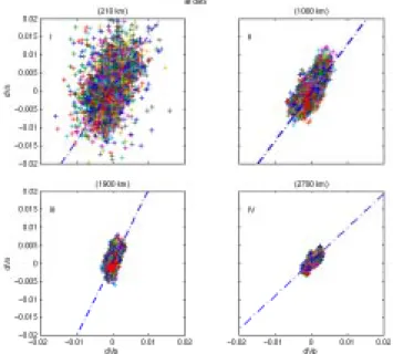
To quantify the correlation between the models and to calculate∂ ln Vs/∂ ln Vpand∂ ln Vφ/∂ ln Vsfor a given region and depth of interest, we plot for each cell the magnitude of the perturbations against one another and determine the slope of the best-fitting line by iterative linear regression (Figure 2). After rescaling the axes according to the results of the noise tests, so that both have similar estimated uncer-tainties, we make an initial guess of the slope and y-intercept and then iteratively refit the line by weighting the perturba-tions that are outside of 1σ by the inverse of their distance from this line. Perturbations within 1σ are weighted equally. This weighting scheme minimizes the effects of outliers and at the same time prevents the data closest to the initial guess from dominating the solution. Unsampled regions are excluded from the analysis.
The bulk-sound errors (σVφ) are inferred from the errors in the P and S wave models according to
σ2 Vφ =σV2p( Vp Vφ) 2+16 9σ 2 Vs( Vs Vφ) 2, (2)
which yields an estimate of bulk-sound model uncertainty of ∼1.2 times the S-wave model.
Results
We find that the P and S-wave models are strongly cor-related at all depths (R∼0.6-0.7) confirming earlier results [Robertson and Woodhouse, 1996; Kennett et al., 1998; Mas-ters et al., 2000]. However, except for the very deep mantle and the top several hundred km near the surface, we find
Figure 2. Plots of P-wave versus S-wave perturbations from each of the four depth ranges. Note how the slope of the fitted line changes with depth.
that through much of the mantle there is no significant cor-relation between the bulk-sound and S-wave perturbations, although the magnitude and slope of the correlation coeffi-cients as a function of depth is similar to that of Masters et al. [2000]. It is possible that this lack of correlation is due to compositional heterogeneity throughout the lower mantle or that the contribution of the bulk modulus is small. It is also possible that our bulk-sound wavespeed model is too noisy for this comparison.
Next, we distinguish regions where there has been sub-duction in the last 120 million years from those where there has not and loosely divide the mantle into four depth inter-vals: I (0-660 km), II (660-1500 km), III (1500-2400 km), and IV (2400-CMB). In the upper mantle (depth I), which is best sampled beneath earthquakes and stations, and the mid-mantle (depth II), which is generally well sampled, we find no significant differences in ∂ ln Vs/∂ ln Vp between re-gions where there has and has not been subduction in the last 120 million years (Figure 3a). However, in the lower mantle the curves have different slopes and begin to diverge at ∼1000 km depth. The lack of a statistically significant difference between the slab and non-slab regions to at least 1200 km depth is consistent with an interpretation that the anomalies have a thermal origin.
0 1 2 3 0 500 1000 1500 2000 2500 depth (km) ∂lnVs/∂lnVp I II III IV slab non−slab −1 0 1 correlation coefficient bulk vs shear compressional vs shear 0 1 2
difference between two regions
Figure 3. (a) S-wave versus P-wave model perturbations in non-slab regions (solid line) versus slab regions (dashed line) as a function of depth. The shaded areas indicate the 1σ uncertainty and encompass the models allowed by the data. (b) Correlation coefficients for bulk and shear (pair on the left) and P and S-waves (pair on the right) as a function of depth. Slab regions shown with dashed and non-slab-regions with solid lines. The gray zone around zero depicts the range within which the correlations are not thought to be significant. Throughout most of the mantle the bulk and shear models are not significantly correlated except for a negative correlation between 1700 and 2400 km depth. The P and S-wave models are positively correlated throughout the mantle. (c) Difference between the slab and non-slab regions for a series of regionalizations shifted by 10 degree intervals around the globe (green). The regionalization shown in Figure 1 is the one that produces the largest difference between the slab and non-slab regions (pink curve) in the lower mantle, demonstrating that the differences are not due to a bias in sampling or random chance.
Between∼1500 and ∼2100 km depth, ∂ ln Vs/∂ ln Vp in-creases slightly in the slab regions and dramatically in the non-slab regions before decreasing (along with data cover-age) toward the core mantle boundary. Previous studies [Robertson and Woodhouse, 1996] found a similar increase in ∂ ln Vs/∂ ln Vp and argued that it results from the in-crease in pressure with depth, which causes a reduction in the sensitivity of the bulk modulus to changes in tempera-ture [Agnon and Bukowinski, 1990; Isaak et al., 1992]. While that effect may be occuring, it is unlikely the dominant fac-tor here because at those same depths we also find the bulk and shear wave perturbations are negatively correlated in the non-slab regions (Figure 3b), which suggests, instead, a predominance of compositional heterogeneity [Stacey, 1998]. In addition to our uncertainty analysis, we conducted two tests to assess the significance and robustness of the result shown in Figure 3a. First, we applied the above analysis to a large number of different regionalizations. Figure 3c shows the result of shifting the slab vs. non-slab regions randomly around the globe. The deep mantle difference in ∂ ln Vs/∂ ln Vppeaks for the regionalization that is based on the actual distribution of slabs, that is, the regionalization as shown in Figure 1. For any other regionalization the
dif-1338 SALTZER ET AL: P AND S WAVE HETEROGENEITY IN THE MANTLE ferences are smaller, except in the shallow mantle. Second,
we have tested whether preferential sampling of low-velocity regions beneath the southern Pacific ocean and Africa as suggested by Masters et al. [2000] could bias our results and found that excluding those regions from the analysis does not significantly change them. These results suggest that the deep mantle difference in ∂ ln Vs/∂ ln Vp between the slab and non-slab regions and the negative correlation in ∂ ln Vφ/∂ ln Vsare robust and causally related to the pattern of subduction in the lower mantle.
The boundary layers (regions I and IV) are another part of the globe where we find significant differences. In the very top of the upper mantle beneath cratons and shields (not shown) we find a negative correlation in∂ ln Vφ/∂ ln Vs
suggesting they are compositionally distinct, in support of the tectosphere hypothesis [Jordan, 1975]. In addition, ∂ ln Vs/∂ ln Vpis significantly higher in both tectonically
ac-tive and young, oceanic regions than in more stable, con-tinental regions, which is consistent with high temperature gradients or the presence of partial melt and volatiles. At the very bottom of the mantle (the lower boundary layer) we find a positive correlation between ∂ ln Vφ/∂ ln Vs, which is consistent with thermal effects at the core-mantle boundary.
Conclusions
The deep mantle (>1000 km depth) beneath regions that have undergone subduction in the last 120 million years have consistently lower ∂ ln Vs/∂ ln Vp ratios than regions that have not. In addition, the largest difference occurs between 1700 and 2400 km depth where a significant nega-tive correlation between∂ ln Vφ/∂ ln Vssuggests widespread chemical heterogeneity. These results do not dictate the na-ture of the compositional heterogeneity and are consistent with mantle models involving anomalous domains, as en-visioned by Kellogg et al. [1999], or slab accumulations, as suggested by Christensen and Hofmann [1994], provided the latter extend far enough above the core mantle boundary.
The boundary layers (regions I and IV) are another part of the globe where we find significant differences. Beneath Pre-cambrian cratons and shields to ∼250 km depth, we find a negative correlation in∂ ln Vφ/∂ ln Vssuggesting com-positional heterogeneity. In tectonically active and young oceanic regions ∂ ln Vs/∂ ln Vp is significantly higher than in more stable, continental regions, consistent with elevated temperature gradients and partial melt or volatiles. We find a positive correlation between∂ ln Vφ/∂ ln Vs at the base of the mantle (the lower boundary layer) which is consistent with thermal effects at the core mantle boundary.
We realize that higher-quality traveltime residuals are necessary to provide a more complete and robust picture. In particular, the S-wave model is less robust than the P-wave model despite similar ray sets, damping etc. which we attribute to lower quality S-wave residuals. Higher-quality S-wave and bulk-sound wavespeed models are required to determine whether the lack of correlation in bulk and shear wavespeed models throughout much of the mantle is due to physical properties in the mantle or is just an artifact of noise in the models.
Acknowledgments. We thank Frank Stacey and Jeannot Trampert for thoughtful reviews of the manuscript. This research was supported by NSF under grant EAR-9905779 and the David and Lucille Packard Foundation.
References
Agnon, A., and M. S. T. Bukowinski, δs at high-pressure and ∂ ln Vs/∂ ln Vp in the lower mantle, Geophys. Res. Lett., 17, 1149-1152, 1990.
Christensen, U. R., and A. Hofmann, Segregation of subducted oceanic-crust in the convecting mantle, J. Geophys. Res., 95, 19,867-19,884, 1994
Engdahl, E. R., van der Hilst, R. D., and R. Buland, Global tele-seismic earthquake relocation with improved travel times and procedures for depth determination, Bull. Seis. Soc. Amer., 88, 72-743, 1998
Jordan, T. H., The continental tectosphere, Rev. Geophys., 13, 1-12, 1975
Isaak, D. G., Anderson, O. L., and R. E. Cohen, The relationship between shear and compressional velocities at high pressures: reconciliation of seismic tomography and mineral physics, Geo-phys. Res. Lett., 8, 741-744, 1992
K´arason, H., and R. D. Van der Hilst, Improving the tomographic imaging of the lowermost mantle by incorporation of differen-tial times of refracted and diffracted core phases (PKP, Pdiff), J. Geophys. Res., in press, 2001
Kellogg, L. H., Hager, B. H., and R. D. van der Hilst, Compo-sitional stratification in the deep mantle, Science, 283, 1881-1884, 1999
Kennett, B. L. N., Engdahl, E. R., and R. Buland, Constraints on seismic velocities in the Earth from traveltimes, Geophys, J. Int., 122, 108-124, 1995
Kennett, B. L. N., Widiyantoro, S., and R. D. van der Hilst, Joint seismic tomography for bulk sound and shear wave speed in the Earth’s mantle, J. Geophys. Res., 103, 12,469-12,493, 1998 Li, X. D., and B. Romanowicz, Global mantle shear velocity
model developed using nonlinear asymptotic coupling theory, J. Geophys. Res., 101, 22,245-22,272, 1996
Masters, G., Laske G., Bolton, H., and A. Dziewonski, The rela-tive behavior of shear velocity, bulk sound speed and compres-sional velocity in the mantle: implications for chemical and thermal structure, Geophys. Mon., 117, 63-87, 2000
Robertson, G. S., and J. H. Woodhouse, Ratio of relative S to P velocity heterogeneity in the lower mantle, J. Geophys. Res., 101, 20,041-20,052, 1996
Stacey, F. D., Thermoelasticity of a mineral composite and a reconsideration of lower mantle properties, Phys. Earth. Plan. Int., 106, 219-236, 1998
Su, W., and A. M. Dziewonski, Simultaneous inversion for 3-D variations in shear and bulk velocity in the mantle, Phys. Earth. Plan. Int., 100, 135-156, 1997
Su, W., Woodward, R. L., and A. M. Dziewonski, Degree 12 model of shear velocity heterogeneity in the mantle, J. Geo-phys. Res., 99, 6945-6980, 1994
Van der Hilst, R. D., and H. K´arason, Compositional heterogene-ity in the bottom 1000 kilometers of Earth’s mantle: toward a hybrid convection model, Science, 283, 1885-1888, 1999 Wen, L., and D. L. Anderson, The fate of slabs inferred from
seismic tomography and 130 million years of subduction, Earth Plan. Sci. Lett., 133, 185-198, 1995
R. L. Saltzer, R. D. Van der Hilst, and H. K´arason De-partment of Earth, Atmospheric and Planetary Sciences, Mas-sachusetts Institute of Technology, Cambridge, MA, 02142. (e-mail: [email protected])
(Received September 14, 2000; revised December 29, 2000; accepted January 15, 2001.)