HAL Id: hal-02167956
https://hal.archives-ouvertes.fr/hal-02167956
Submitted on 28 Jun 2019
HAL is a multi-disciplinary open access
archive for the deposit and dissemination of
sci-entific research documents, whether they are
pub-lished or not. The documents may come from
teaching and research institutions in France or
abroad, or from public or private research centers.
L’archive ouverte pluridisciplinaire HAL, est
destinée au dépôt et à la diffusion de documents
scientifiques de niveau recherche, publiés ou non,
émanant des établissements d’enseignement et de
recherche français ou étrangers, des laboratoires
publics ou privés.
Performance evaluation of solar energy predictor for
wireless sensors
Bingying Li, Yuehua Ding, Yanping Wang
To cite this version:
Bingying Li, Yuehua Ding, Yanping Wang. Performance evaluation of solar energy predictor for
wire-less sensors. Fifth Sino-French Workshop on Information and Communication Technologies (SIFWICT
2019), Jun 2019, Nantes, France. �hal-02167956�
Fifth Sino-French Workshop on Information and Communication Technologies
SIFWICT 2019 - June 21, 2019, Nantes, France
Direction-of-Arrival Estimation Using Co-prime
Array in the Context of Both Circular and
Non-circular Sources
Bingying LI,
Yuehua DING
School of Electronic and Information Engineering South China University of Technology
Guangzhou, China eeyhding@scut.edu.cn
Yide WANG
IETR, UMR 6164, School of Polytech’ Nantes University of Nantes
Nantes, France Yide.wang@univ-nantes.fr
Abstract—Recently, coprime array has been proposed to
es-timate the direction of arrival (DoA) of O(M N ) sources using only O(M + N ) physical sensors. In this paper, we investigate a new method to achieve higher degrees of freedom for the coprime array under the coexistence of K1non-circular and K2 circular
sources. By exploiting the properties of the signal sources, a new model is constructed based on a longer virtual uniform linear array (ULA). Simulation results show that the proposed method can identify more sources once the condition K1+ 2K2< 2M N
is satisfied.
Index Terms—DoA estimation, coprime array, MUSIC, non
circularity and circularity.
I. INTRODUCTION
Direction of arrival (DoA) estimation plays a significant role in array signal processing. It has wide application in many fields such as radar, sonar and wireless communication systems [1] - [3]. During the past several decades, research in DoA estimation of narrowband signals has achieved a huge progress since the multiple signal classification (MUSIC) [4] was proposed. Its mainstream is focused on half wave length spaced uniform linear arrays (ULA). It is well known that the resolution capability of a ULA is directly limited by the number of its physical sensors. For example, with a ULA of
N sensors, the number of resolvable uncorrelated sources by
MUSIC-like algorithms is N − 1.
To overcome the above mentioned limitation, coprime array has been recently proposed, which is a non-uniform linear array constituted of two uniform linear subarrays with large inter-element distances [5]. This new geometry shape can increase the degrees of freedom of the array by exploiting the covariance matrix of the received signals. A new system model can be obtained by vectorizing the covariance matrix of the received signals. It can be viewed as a virtual ULA with a much wider aperture, which is able to detect O(M N ) sources using only O(M + N ) physical sensors. The spatial smoothing method is then used to overcome the correlation effect [6]. Actually, this method has been widely applied in many systems to get further improvements in sources’ DoA
finding [7] - [9].
Moreover, researchers are also interested in the exploitation of the properties of incoming signals which can bring further estimation improvement. When the incoming signals are from non-circular sources, the DoA estimation accuracy and the maximum number of detectable signals can be greatly increased [10]. [11] developed an algorithm to cope with more general scenarios, where the non-circular and circular sources are mixed together. It can make use of the existing non-circular signals to increase the maximum number of detectable signals. It combines the received signal vector and its complex conjugate counterpart to form a new signal vector and exploits the covariance matrix of the new signal vector. It also proposes different estimators for non-circular sources and for circular sources to achieve higher accuracy.
For the coprime arrays, the property of non-circular signals is exploited in [12] to enhance the DoA finding performance, while the case of mixed signals including non-circular and circular signals is still not investigated. Motivated by this observation, in this paper, we make use of coprime array and exploit the properties of real and complex circular sources to increase the degrees of freedom in DoA estimation. The rest of this paper is organized as follows: Section II presents the MUSIC-based DoA estimation for a classical ULA, then for a coprime array. The proposed method is presented in Section III. Simulation results are provided in section IV. Section V concludes the paper.
Notation: Capital letters of boldface are used for matrices.
Lowercase letters of boldface denote column vectors. (·)Hand
(·)T denote the operations of Hermitian (complex conjugate
transpose) and transpose, respectively. The operation of
com-plex conjugate is denoted by (·)∗. E[·] denotes the expectation.
∥ · ∥ represents the Frobenius norm. ⊗ denotes the Kronecker
product. Diagonal matrices are denoted by diag(·). j is used
the M × M identity matrix. 0 represents a zero matrix or vector.
II. PROBLEMFORMULATION
A. Classical model
Consider a ULA of M sensors with d the distance between two adjacent sensors. Suppose K uncorrelated narrowband
sources impinging on this array from directions θk, k =
1, . . . , K. The used snapshots number is denoted by N . The received signal at the array sensors is the superposition of these signals, which can be expressed as:
x(t) = As(t) + n(t) (1)
where A = [a(θ1), . . . , a(θK)]; s(t) = [s1(t), . . . , sK(t)]T;
n(t) represents the spatially and temporally white noise; sk(t)
denotes the k-th signal received at the first sensor; n(t) and
s(t) are assumed to be uncorrelated and a(θk) is the steering
vector corresponding to sk(t), given by
a(θk) = [1, ej
2π
λdsinθk, . . . , ej(M−1)2πλdsinθk]T λ is the wavelength of the impinging narrowband signals, and d is usually set to be λ/2.
B. MUSIC algorithm
The correlation matrix of the received signal in (1) can be expressed as Rxx= E[x(t)xH(t)] = AE[s(t)sH(t)]AH+ σn2IM = ARssAH+ σ2nIM = UΛUH+ GΓGH (2)
where the columns of U generate the signal-subspace, formed by the eigenvectors corresponding to the K largest eigenvalues and the columns of G span the noise-subspace, formed by the
eigenvectors corresponding to the M−K smallest eigenvalues.
Since the signal-subspace and noise-subspace are orthogonal,
the actual source steering vector a(θk) and the noise-subspace
are orthogonal.
a(θk)HG = 0, f or k = 1, 2, . . . , K (3)
Therefore, the spatial pseudo-spectrum can be expressed as
p(θ) = 1
a(θ)HGGHa(θ) (4)
C. Coprime array
Assume N and M are two coprime numbers. Consider a
linear array with N + 2M− 1 non-uniformly located sensors
along the X-axis, whose positions are given by the following set in terms of X-coordinate:
S ={Mnd, 0 ≤ n ≤ N − 1}∪{Nmd, 1 ≤ m ≤ 2M − 1}
0 Md 2Md (N-1)Md
Nd 2Nd (2M-1)Nd ĂĂ
ĂĂĂĂ
Fig. 1. Coprime array.
where, d is the fundamental spacing.
Similar to model (1), the received signal is denoted by
x(t) = As(t) + n(t) (5)
where a(θ) is the (N + 2M− 1) × 1 steering vector whose
elements are given by
ej2πλlsinθ, l∈ S
The correlation matrix of the received signal is given by:
Rxx= E[x(t)xH(t)] = ARssAH+ σn2IN +2M−1 = K ∑ i=1 σi2a(θi)aH(θi) + σ2nIN +2M−1 (6)
Since the sources are temporally uncorrelated, Rss is a
di-agonal matrix with didi-agonal elements σ2
1, σ22, . . . , σK2 which
are equal to the actual sources powers. By vectorizing the
correlation matrix Rxx. The following vector is obtained:
z = vec(Rxx) = vec[ K ∑ i=1 σ2ia(θi)aH(θi)] + σn2˜ln = B(θ1, . . . , θK)p + σn2˜ln (7)
where B(θ1, . . . , θK) = [a∗(θ1)⊗a(θ1), . . . , a∗(θK)⊗a(θK)],
p = [σ2
1, σ22, . . . , σK2] T
, and ˜ln = [eT1, eT2, . . . , eTN +2M−1] T
with ei a column vector of all zeros, except the one at the
i-th position, which is equal to one. Comparing (7) with (1),
z behaves like a signal vector received by a longer virtual array and B acts as the manifold matrix. The equivalent source signal vector is represented by p and the noise becomes
a deterministic vector given by σn2˜ln. According to B, the
locations of the virtual sensor array are given by the values in the following set including the subset of cross differences
{±(Mn − Nm)d, 0 ≤ n ≤ N − 1, 1 ≤ m ≤ 2M − 1} and
the subset of self-differences{(Mn1− Mn2)d, 0≤ n1, n2≤
N−1}, {(Nm1−Nm2)d, 1≤ m1, m2≤ 2M −1}. It includes
2M N + 1 consecutive differences from−MNd to MNd [5].
By extracting and sorting those rows corresponding to the 2M N + 1 consecutive differences, a new model is obtained as follows:
˜
where ˜e′is a vector of all zeros except a ”1” at the (M N +1)-th position. (8) is equivalent to a ULA receiving K coherent
sources p with deterministic noise term σn2e˜′. By applying
MUSIC with spatial smoothing, it can identify M N sources.
III. PROPOSED METHOD FOR MIXED SIGNALS
Recently, [12] proposed a method to enhance the DoA finding performance for non-circular signals by using coprime array. In this paper, we extend the discussion to the mixed signals including non-circular and circular signals.
A. Data model
Consider the model in (5), assume K temporally uncorrelat-ed narrowband signals are impinging on this array from
direc-tions{θi, i = 1, 2, . . . , K} with powers {σi2, i = 1, 2, . . . , K},
in which there are K1 non-circular signals and K2 circular
signals, respectively, K = K1+ K2. Equation (5) can be
rewritten as:
x(t) = As(t) + n(t) = A1snc(t) + A2sc(t) + n(t) (9)
where A = [A1, A2] with A1 = [a(θ1), a(θ2), . . . , a(θK1)]
and A2= [a(θK1+1), a(θK1+2), . . . , a(θK1+K2)] denoting the
array manifold matrices, and snc(t) and sc(t) denoting the
non-circular real signals and complex circular signals respec-tively. n(t) represents the spatially and temporally white noise, which is uncorrelated with the sources. By combining the original signal vector and its complex conjugate counterpart, a new extended signal model can be formed:
˜ x = [ x(t) x∗(t) ] = [ A1 A∗1 ] snc+ [ A2 0 0 A∗2 ][ sc(t) s∗c(t) ] + [ n(t) n∗(t) ] (10) B. Co-array model
Based on model (10), we get the correlation matrix of the extended received signal:
Rx˜˜x= E[˜x˜xH] = [ E[x(t)xH(t)] E[x(t)xT(t)] E[x∗(t)xH(t)] E[x∗(t)xT(t)] ] (11)
Considering the fact that the signals are uncorrelated with each other and with the noise, and that both the mean and the elliptic covariance of a circular signal are equal to zero,
we have E[sisTi ] = E[s∗isHi ] = 0, for K1+ 1≤ i ≤ K1+ K2,
and the following equations hold:
E[x(t)xH(t)] = K ∑ i=1 σi2a(θi)aH(θi) + σ2nIN +2M−1 (12) E[x(t)xT(t)] = K1 ∑ i=1 σ2ia(θi)aT(θi) (13) E[x∗(t)xH(t)] = K1 ∑ i=1 σi2a∗(θi)aH(θi) (14) E[x∗(t)xT(t)] = K ∑ i=1 σ2ia∗(θi)aT(θi) + σn2IN +2M−1 (15)
Next, we vectorize these four parts of R˜x˜xto get the following
vectors: z1= vec(E[x(t)xH(t)]) = B1(θ1, . . . , θK1+K2)p1+ σ 2 n˜ln (16) z2= vec(E[x(t)xT(t)]) = B2(θ1, . . . , θK1+K2)p2 (17) z3= vec(E[x∗(t)xH(t)]) = B3(θ1, . . . , θK1+K2)p3 (18) z4= vec(E[x∗(t)xT(t)]) = B4(θ1, . . . , θK1+K2)p4+ σ 2 n˜ln (19) The following extended model can be obtained by stacking z1, z2, z3 and z4: z = [zT1, zT2, zT3, zT4]T = Bp∗+ σ2nζ˜n (20) where B = [BT 1, BT2, BT3, BT4] T , with B1(θ1, . . . , θK1+K2) = [a∗(θ1)⊗ a(θ1), . . . , a∗(θK1+K2)⊗ a(θK1+K2)], B2(θ1, . . . , θK1+K2)
= [a(θ1)⊗ a(θ1), . . . , a(θK1+K2)⊗ a(θK1+K2)],
B3(θ1, . . . , θK1+K2) = [a∗(θ1)⊗ a∗(θ1), . . . , a∗(θK1+K2)⊗ a∗(θK1+K2)], B4(θ1, . . . , θK1+K2) = [a(θ1)⊗ a∗(θ1), . . . , a(θK1+K2)⊗ a∗(θK1+K2)]; p∗= [pT1, pT2, pT3, pT4]T, with p1= p4= [σ12, σ22, . . . , σK21+K2] T , p2 = p3 = [σ21, σ22, . . . , σK21, 0, . . . , 0] T
in which there are
zeros for the last K2 elements; and ˜ζn = [˜lTn, 0
T, 0T,˜lT n]
T,
˜ln = [eT1, eT2, . . . , eTN +2M−1] T
with ei denoting column
vector of all zeros, except the one at the i-th position, which is equal to one, and 0 represents a zero column vector
with the same size as ˜ln. Similar to Section II-C, Bi can
be regarded as a manifold matrix and the corresponding
equivalent source signal vector is represented by pi, while
the noise becomes a deterministic vector.
The distinct rows of B1and B4behave like the manifold of
a longer array whose sensor locations are given by the values
in the set including the subset of cross differences{±(Mn −
N m)d, 0≤ n ≤ N − 1, 1 ≤ m ≤ 2M − 1} and that of
N m2)d, 1≤ m1, m2≤ 2M − 1}. This set includes 2MN +
1 consecutive differences from −MN to MN. The sensor
positions represented by the rows of B2 and B3are given by
the set including subset{±(Mn+Nm)d, 0 ≤ n ≤ N −1, 1 ≤
m≤ 2M − 1}, {(Mn1± Mn2)d, 0≤ n1, n2≤ N − 1} and
subset {(Nm1± Nm2)d, 1≤ m1, m2≤ 2M − 1}.
The positions of the virtual sensors include more than
4M N + 1 consecutive differences. Hence from Bi, for
non-circular signals, we can extract a manifold matrix of
a much longer ULA with 2Mmax + 1 sensors located at
nd,−Mmax≤ n ≤ Mmax, where Mmax> 2M N .
By extracting and sorting those rows from B which
corre-spond to the 2Mmax+ 1 consecutive sequence, we construct
a new matrix M of size (2Mmax+ 1)× K. The (n, i)−th
element of M is given by ej2nπdsinθi/λ, i = 1, 2, . . . , K, n =
−Mmax,−Mmax + 1, . . . ,−1, 0, 1, . . . , Mmax− 1, , Mmax.
This is equivalent to extracting and sorting the corresponding
rows from the observation vector z to form a new vector ˜z:
˜
z = Mp∗+ σn2e˜′
where ˜e′∈ R(2Mmax+1)×1 is a vector of all zeros except a 1
at the (Mmax+ 1)-th position. The vector ˜ζn consists of 0s
and 1s with the 1s occurring exactly at those rows where the phase terms in B are equal to 0. Therefore, corresponding to
the center row, the (Mmax+ 1)th element of ˜e′ is equal to
1. M is exactly identical to the manifold matrix of an ULA
with 2Mmax+ 1 sensors located from −Mmaxd to Mmaxd.
C. Spatial smoothing
For ˜z, it consists of the powers of the actual sources
behaving like fully coherent sources, spatial smoothing is
needed. We divide the virtual ULA with 2Mmax+ 1 sensors
into Mmax+ 1 overlapping subarrays, each with Mmax+ 1
elements, where the th subarray corresponding to the
i-th to i-the (Mmax+ i)-th rows of ˜z has sensors located at
{(n+i−Mmax)d, n = 0, 1, . . . , Mmax}. We denote the signal
received by the i-th subarray as ˜
zi= Mip∗+ σ2ne′i (21)
where Mi is a (Mmax+ 1)× K matrix taking the elements
from the i-th to the (Mmax+ i)-th rows of M and e′i is a
vector of all zeros except a ”1” at the (Mmax + 2− i)-th
position. Define Ri = ˜zi˜zHi . Taking the average of Ri over
all i, we get Rs = 1 Mmax+ 1 Mmax∑+1 i=1 Ri (22)
Since Mmax > 2M N , Rs is the spatially smoothed matrix
with which we are able to estimate the DoA of up to 2M N non-circular sources or M N circular sources. As for
mixed source signals, it can identify K1+ K2 sources once
K1+ 2K2< 2M N is satisfied.
D. Estimating method
Rsis a full rank matrix and the eigendecomposition can be
applied as
Rs = UΛUH+ GΓGH (23)
where the diagonal matrix Λ of (K1+ 2K2)× (K1+ 2K2)
contains the K1+ 2K2 eigenvalues of Rs and the diagonal
matrix Γ contains the Mmax− K1− 2K2 eigenvalues of Rs.
According to [11], we partition G as G = [GT1, GT2]
T
where
G1and G2are two matrices with equal dimension. In general,
we can use (24) to estimate the DoA of each signal as follows:
f (θ) = 1
a(θ)HGGHa(θ) (24)
To improve the estimation performance for circular signals, (25) is employed as follows: fc(θ) = 1 a(θ)HG 1GH1 a(θ) (25)
IV. SIMULATIONRESULTS
In this section, simulation is performed to examine the performance of the proposed method in 3 different cases. In the simulation, we assumed M = 5, N = 7, the fundamental spacing d = λ/2.
A. Case I: circular signals
In this case, we consider D = 35 circular signals with DoAs
θ uniformly distributed from sin(θ) =−1 to sin(θ) = 1. The SN R is set to be 0 dB using 3000 snapshots. With M = 5 and N = 7, we can estimate up to M N = 35 sources from distinct
directions. Fig.2 shows the MUSIC spectrum. Apparently, it can identify all the DoAs clearly.
sin(θ) -1 -0.8 -0.6 -0.4 -0.2 0 0.2 0.4 0.6 0.8 1 Log(Steered Response) -18 -16 -14 -12 -10 -8 -6 -4 -2 0
Fig. 2. Spectrum for DOA estimation of circular signals using proposed method,M=5,N=7,SNR=0dB.
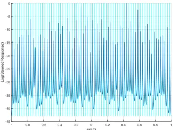
B. Case II: real signals
For the real signal case, we use D = 70 real signals with
DoAs θ uniformly distributed from sin(θ) =−1 to sin(θ) =
1. The SN R is set to be 0 dB. 1000 snapshots is used, M = 5 and N = 7. Fig.3 shows that the proposed method can identify 70 sources clearly, which is 2 times more than the traditional MUSIC based on coprime array.
sin(θ) -1 -0.8 -0.6 -0.4 -0.2 0 0.2 0.4 0.6 0.8 1 Log(Steered Response) -45 -40 -35 -30 -25 -20 -15 -10 -5 0
Fig. 3. Spectrum for DOA estimation of real signals using proposed method,M=5,N=7,SNR=0dB.
C. Case III: co-existence of circular and non-circular signals
As for the mixed signals, we consider K1= 30 non-circular
signals and K2= 10 circular signals with M = 5 and N = 7.
The SN R is set to be 0 dB. 3000 snapshots are used in simulation. Fig.4 shows that the proposed estimator is able
sin(θ) -1 -0.8 -0.6 -0.4 -0.2 0 0.2 0.4 0.6 0.8 1 Normalized spectrum) 0 0.1 0.2 0.3 0.4 0.5 0.6 0.7 0.8 0.9 1
DoA of all signals by (24) DoA of circular signals by (25)
Fig. 4. Spectrum for mixed signals using proposed method.
to identify both non-circular signals and circular signals with good accuracy.
V. CONCLUSIONS
In this paper, a new DOA estimation method is proposed
for the co-prime array in the context of K1 non-circular
and K2 circular sources. Simulation results shows that the
proposed method increases degrees of freedom greatly and distinguish the circular signal and the non-circular signal
clearly once the condition K1+ 2K2< 2M N is satisfied.
REFERENCES
[1] G. Zheng, B. Chen, and M. Yang, ”Unitary ESPRIT algorithm for bistatic MIMO radar,”Electronics Letters, vol. 48, no. 3, pp. 179-181, Feb. 2012.
[2] R. Cao, B. Liu, F. Gao, and X. Zhang, ”A low-complex one-snapshot DOA estimation algorithm with massive ULA,” IEEE Communications Letters, vol. 21, no. 5, pp. 1071-1074, May 2017.
[3] M. Jiang, J. Huang , W. Han , F. Chu . ” Research on target DOA estimation method using MIMO sonar,” IEEE Conference on Industrial Electronics & Applications. IEEE, pp. 1982-1984, Jun. 2009. [4] R.O. Schmidt, ”Multiple emitter location and signal parameter
estima-tion,” IEEE Transactions on Antennas and Propagation, vol. 34, no. 3, pp. 276-280, Mar. 1986.
[5] P. Pal and P. P. Vaidyanathan, ”Coprime sampling and the music algorithm,” Digital Signal Processing and Signal Processing Education Meeting (DSP/SPE), pp. 289-294. Mar. 2011.
[6] T. J. .Shan ”On Spatial Smoothing for Direction-of-Arrival Estimation of Coherent Signals,” IEEE Transactions on Acoustics, Speech, and Signal Processing, Vol. ASSP-33, NO. 4, pp. 806-811, Aug. 1985
[7] J. Li, M. Shen, D. Jiang, ”DOA estimation based on combined ESPRIT for co-prime array,” IEEE Conference on Antennas & Propagation. IEEE, pp. 117-118, Feb. 2017.
[8] A. Nguyen, T. Matsubara, and T. Kurokawa, ”High-Performance DOA Estimation for Coprime Arrays with Unknown Number of Sources,” Asia-Pacific International Symposium on Electromagnetic Compatibility (APEMC), pp. 369-371, Jun. 2017.
[9] J. Li, D. Li, D. Jiang, and X. Zhang, ”Extended-Aperture Unitary Root MUSIC-Based DOA Estimation for Coprime Array,” IEEE Communi-cations Letters, Vol. 22, no. 4 pp. 752-755, Apr. 2018
[10] P. Charge, Y. Wang, and J.Saillard, ”A root-music algorithm for non circular sources,” 2001 IEEE International Conference on Acoustics, Speech, and Signal Processing, vol. 5, pp. 7-11, May 2001.
[11] F. Gao, A. Nallanathan, Y. Wang, Improved MUSIC Under the Coexis-tence of Both Circular and Noncircular Sources, IEEE Transactions on Signal Processing, vol. 56, no. 7, pp. 3033-3038, Jul. 2008.
[12] H. Zhai, X. Zhang, W. Zheng, and P. GONG, ”DOA Estimation of Noncircular Signals for Unfolded Coprime Linear Array: Identifiability, DOF and Algorithm(May 2018),” IEEE Access, Vol. 6, pp. 29382-29390, May 2018.