The Design of Intergovernmental Equalisation Transfers: Indian States and Kosovo

The Design of Intergovernmental Equalisation Transfers: Indian states

and Kosovo

By

January 2007

MSc Essay, sciences économiques ,Université de Montréal

1

I wish to thank François Vaillancourt for research supervision 2

Introduction

This essay examines how to design intergovernmental equalisation transfers (IET) for two cases. The first is the case of Indian states where we examine how the use of imperfect data can efficiently approximate first-best measures of fiscal capacity and optimal IET schemes. The second is the case of Kosovo where we will simulate an IET scheme using property tax data.

The purpose of the first part of this paper is to examine how a number of imperfect indicators usually available in developing countries compare to a first-best measure of fiscal capacity. This is of interest since economists working in the field of fiscal federalism often have to conceive intergovernmental equalisation transfers (IET) schemes in countries where the appropriate data required for optimal design is not available. This paper follows two prior studies that sought to answer the same question: Vaillancourt (2001) and Boex and Martinez-Vazquez (2004). Our analysis was carried out using a World Bank study of local organizations in India which provides us with data that both is and is not usually available in developing countries.

In the second part of this paper we will devise an IET scheme for Kosovo using recent data on tax assessment as a proxy for fiscal capacity. Limited data availability had prevented ed the country from having a proper IET scheme for a number of years.

The paper is divided into three sections. We first review the theoretical and empirical literature on IET in section 1. In the second section, we present the data and related issues, discuss our methodology and examine the results for the Indian case and then conclude. In the third and last section of this paper, we look at the case of Kosovo. We present the data and methodology. The results are discussed. Lastly, we conclude briefly.

1. What are IET ?

Equalisation consists of a system of unconditional redistributive transfers usually from the central to sub-national governments (SNGs), hence the name intergovernmental equalisation transfers (IET). The main purpose of such transfers is to enable SNGs with different revenue raising capabilities (fiscal capacity) and different expenditure needs (fiscal needs) to provide comparable levels of public services at comparable revenue efforts. In other words, such transfers aim to equalise the net fiscal benefit (NFB) received by otherwise-equal individuals in different regions of a single country; where NFB equals the amount of public services received minus the amount of taxes paid.

i i i

NFB = public services received −taxes paid

IET are a consequence of decentralisation. That is, IET are needed to replicate the fiscal structure of unitary state within a decentralised federation. The question of whether IETs are desirable is a matter for societal consensus and subsequent policy choices. This paper will not examine the case for desirability. Rather, this paper assumes such equalisation schemes are desirable.

Since James Buchanan’s influential paper (1950) a significant literature has developed on the use of IET to rectify inequities and inefficiencies that may arise within a decentralised federation. Indeed, Buchanan and many others3 (Boadway and Flatters, Shah) argue that IET constitute a rare occurrence in economics, i.e., it is the case where both equity and efficiency concerns coincide. This section will provide a brief overview of this literature4.

Equity

Buchanan’s approach focuses solely on the fiscal capacity of SNGs. The fiscal capacity of a SNG is defined as its ability to raise revenues from its particular tax bases.

3

See Buchanan (1950), Boadway and Flatters (1982), Shah (1994) 4

Regarding equity, IET aim to enable SNGs with different fiscal capacities to provide comparable levels of public services at comparable tax rates. In a country with heterogeneous regions, SNGs will likely have different fiscal capacities and as a result will be unable to offer the same level of public services at the same tax rates.

Consequently, to ensure that the same level of public services will be available, the poorer SNGs must impose greater tax burdens on its citizens.

Buchanan focuses exclusively on the “taxes paid” part of the NFB equation. This approach ignores the fact that heterogeneous regions may have inherent characteristics that render them unable to provide certain public services at the same costs. Thus, with respect to IET design one must also take into account the public services received part of the equation which in practice is assessed by indicators of fiscal needs. With heterogeneous regions, fiscal needs differentials may lie in cost differences or needs differences. That is, differences may exist in the per-unit cost or in the number of units needed per capita of a standardised public service. The former may arise from climatic and geographic features or density and distance factors whereas the latter may be due to demographic factors such as the age structure of the population or cultural factors such as the need to provide public services in multiple languages. Thus, IET design should be predominantly concerned with eliminating differences in NFB provided to otherwise-identical individuals living in different regions rather than focusing just on fiscal capacity or fiscal needs.

Efficiency

With respect to efficiency, IET aim to eliminate migration of labour and capital induced by regional differences in NFBs induced by decentralisation. Indeed, economic efficiency requires that the geographical distribution of labour and capital be based on productivity considerations, not on expected NFB.

IET around the world

Many countries opt for a decentralised structure of governance and attempt to implement effective equalisation transfer schemes. For instance, India has used since 1919 a system of intergovernmental fiscal transfers to rectify horizontal and vertical inefficiencies between states5. In India, as it is the case for a number of countries, decision-making over intergovernmental transfers is delegated to an independent agency. In this case, India’s Finance commission provides formulae-based6 equalisation transfers using fiscal capacity, expenditure differential and fiscal effort indices: For the 2000-2005 period, 62.5 percent is based on income per capita, 10 percent is based on population, 7.5 percent on area, 7.5 percent on an index of infrastructure, 7.5 percent on “fiscal discipline” and 5 percent on tax effort. Many other countries have opted for equalisation schemes (e.g. Brazil, China, Malaysia, and Nigeria). Consider Table A-1 from Bird & Vaillancourt (2004). This table shows the importance of IET around the world as well as the diversity of equalisation schemes. However in most developing countries the necessary data to compute IET using formulae-based instruments are rather limited or simply unavailable. How can such countries make an optimal design? This is a question that we and other researchers seek to answer.

When countries opt for equalisation, efficient formulae and indicators are needed. However, in developing countries, it is often the case that the data needed to compute such transfers are limited or unavailable. This has motivated authors (Vaillancourt, 2001 Martinez-Vazquez and Boex, 2004) to find indicators among the available data that best fit the first-best measures of fiscal needs and fiscal capacity.

Vaillancourt’s paper (2001) is a first attempt at examining the way in which various indicators typically prevalent in developing countries are correlated to an indicator of fiscal capacity. To do so, the author used data from the 1951 and 1961 censuses and from 1954 taxation data for the two poorest Canadian provinces, Newfoundland and Prince-Edward-Island. According to Vaillancourt, this data can serve

5

See Rao (2004) p.16 6

as a reasonable proxy for a middle-income developing country such as Morocco. Eight simple indicators are computed:

Demographic indicators

- percentage of the population under age 19 attending school - percentage of the population with little schooling

- percentage of rural population

Housing indicators

- housing in need of repair - wood used for heating fuel - wood or coal used for cooking - households with no piped water

Labour market indicator

- percentage of the population 14 years and older employed

These indicators are computed for each of the thirteen census divisions examined. Both the mean and maximum value of a given indicator are used as targets for equalisation. As a measure of fit, the author reports the absolute difference between the equalisation entitlement obtained for indicator i and the reference point, i.e., an indicator of taxable capacity for each SNG; in this case taxable income. Although no indicator is clearly more precise than another, indicators of rurality (percentage of rural population, percentage with no piped water) perform fairly well. The paper’s main finding is that using maximum rather than mean values as equalisation targets yields better results, since the need to correctly match transfers equal to zero is reduced.

Martinez-Vazquez and Boex proposed a similar analysis. Based on data available for Georgia for 1957-1960 they were able to compute a variety of indicators.

Eight measures of local fiscal needs:

- actual and lagged local expenditures per capita - equal per capita expenditure norm

- the proportion of poor households

- the proportion of households without piped water - an index of need based on infant mortality

- an index of expenditure needs based on poverty, water access and infant mortality (similar to HDI)

- a traditional Representative Expenditure System - a regression-based Representative Expenditure System

They also provide measures of fiscal capacity:

- revenue collection and lagged revenue collection per capita - poverty as a proxy of fiscal capacity

- regional income level as a proxy of fiscal capacity - average per capita personal income

- traditional Representative Revenue System - regression-based Representative Revenue System

The regression-based Representative Expenditure System (and the regression-based RRS) is a data-intensive method based on regression analysis. It involves regressing different expenditure categories on a series of explanatory variables (land area, population, age distribution, etc…) in order to obtain equations for every expenditure category and every SNG. According to the authors, these are the first-best measures of fiscal capacity and fiscal needs.

With respect to fiscal needs, the authors find that the best performing alternative measure is the per capita expenditure norm, which is solely allocated in proportion to population. As it was the case for Vaillancourt, composite indices perform fairly poorly. With respect to fiscal capacity, all the proposed indicators performed well.

The authors conclude rather tentatively. First, different methodologies can have a great impact on IET design. Second, their analysis shows that the best indicators of fiscal needs and fiscal capacity are not necessarily data-intensive. For instance, the per capita

expenditure norm is one of the best-performing indicator and its formula relies only on two variables. Finally, the best performing indicators are both the actual expenditures and revenue collections per capita. But these do not satisfy an incentives criterion which we will discuss later on.

2. India

Data

The data used to perform this analysis came from the World Bank (2001) study of the performance of local organizations in India. The study used a mixed methodology comprised of traditional extensive data collection based on questionnaires and intensive enquiry using interactive methods such as focus groups and various rural appraisal instruments. It aimed to assess the performance of local organizations (LO) that provide development programs in the three key sectors of watershed development (natural resource management), rural water supply and sanitation (basic needs) and rural women empowerment and development (social development).

By means of both quantitative and qualitative methodologies, data were gathered from representatives and staff of LOs implementing such programs; from the villages and elected bodies; and from households benefiting from development programs. The study was conducted in the three states of Karnataka, Madhya Pradesh, and Uttaranchal (formerly Uttar Pradesh) although due to missing data only Karnataka is included in our analysis. We will discuss this point later on.

Respondents for the household questionnaire were selected using a stratified random sample from a listing of members of sector specific local organizations. These organizations were identified during an organizational mapping of each village studied. It is important to point out that villages were not selected at random. Rather, these entities were selected based on the prevalence of sector specific LOs operating within their territory. Therefore, it is unclear whether our results are applicable to the general case. We discuss this point in the next section.

The main issues are twofold. First of all, there is missing or suspicious data for some of the variables in the World Bank study. Second, selection of villages based on the prevalence of LOs within their territory could induce a bias.

Because of missing data on revenues and lagged revenues many observations on villages had to be dropped. In some cases, the data were suspicious showing great variations from year to year. In other cases, the data showed patterns that raised doubts on data collection itself. Thus, many villages were dropped from the sample. The original dataset contained data on 36 villages in Karnataka. After data cleaning only 28 villages were available for analysis. Additionally, there was missing or suspicious data for actual and lagged revenue collections and other variables for villages in Uttaranchal and Madhya Pradesh. Because of this limited availability only the state of Karnataka was included in the final sample.

Table 1 - Original and Final Sample Size by State

State Original Sample Size Final Sample Size

Karnataka 36 28

Uttaranchal 36 0

Madhya Pradesh 36 0

Source: WB Data on the performance of local organisations

Second, as noted above village selection in the World Bank study based on the prevalence of sector specific LOs operating within their territory. Since villages were not selected at random, it is unsure whether our results can be representative of villages without important LO activity. However, the similarity of results to those found in prior studies lessens this concern. Nevertheless, the reader should be warned of such a possibility.

Methodology

We draw on the above-mentioned studies to compute sixteen indicators; their values are reported in table A-2.

- average total income (first-best measure)

- population (distribution based solely on population share) - average revenue collections per capita for each village

- average lagged revenue collections per capita for each village (revenues for the preceding year)

- percentage of poor households

- percentage of households with a water connection

- percentage of households where a child was sick in the last six months - percentage of households who own a television set

- percentage of households who own a radio - percentage of households who own a wall clock - percentage of households who own land

- percentage of households who own an iron box

- percentage of households who own sheep and/or goats - distance (in meters) from the nearest water source - percentage of population that is literate

Revenues and lagged revenues per capita provide information about revenue collections for the Gram Panchayat (government body) from 1998 to 2001 for every village. Since revenues and lagged revenues have proved to be successful indicators for Martinez-Vazquez and Boex, villages for which this data was missing were excluded from the analysis. However, this type of indicator is clearly inefficient from an incentives stand point. Indeed, should IET be based on such indicators SNGs would clearly be inclined to spend more and to minimise tax effort in order to receive more transfers.

As mentioned in the introduction regression-based RRS is argued by Boex and Martinez-Vasquez to be the best available measure of fiscal capacity (regression-based RES is argued to be the best available measure of fiscal needs). However, it is also the

most data-intensive. Ideally, these regression-based methods should be computed using time series data. However, in the World Bank study data on expenditure and revenues was only available for three fiscal years, 1998-1999, 1999-2000 and 2000-2001. Given this limited availability, neither RRS nor RES can be obtained by regressing expenditures categories on a series of factors such as population and land area.

Method

A transfer pool (1 000 000 R’s) is to be allocated between villages (SNGs) using average total income as our first-best indicator. The formula for a given indicator and village i: 1 * * * i i i n i i i TP SharePop ShareDev Allocation SharePop ShareDev = =

∑

Where TP stands for transfer pool, SharePopi is for the share of the total population for village i and ShareDevi is for the share of the sum of the deviations for villages 1…, n from the equalisation target. The same formula is used to compute the allocation of this transfer pool for each of the fifteen remaining indicators. We use both the maximum and the mean value of a given indicator as targets for equalisation. For example, to obtain the allocation for village i we first calculate the total population which is the sum of the population for all villages.

28 1

i

Total Population population of village i

= =

∑

28 1 i i population of village i SharePop population of village i = =

∑

For a given indicator, we then choose an equalisation target - either the mean or the maximum value of the indicator – and obtain the deviation from this target for every village in the sample. By definition, when the maximum value is used, one deviation will equal zero whereas with the use of the mean value, deviations can be either negative,

positive or zero. Villages for which the observed value of an indicator exceeds its mean – with positive deviations - do not receive transfers. The values of their deviations are set to zero. We then compute the absolute value of the sum of the modified deviations.

28 1

i

Total Deviation deviation for village i

= =

∑

We then obtain the share of this sum for village I

28 1

i

i

deviation for village i ShareDev

deviation of village i

= =

∑

We multiply the amount of the transfer pool by these two shares. We compute the sum of the product of these two shares to ensure that the proportions sum to one.

1 * * * i i i n i i i TP SharePop ShareDev Allocation SharePop ShareDev = =

∑

Finally, the allocation produced by each indicator is compared with the first-best indicator (average total income) by computing the total absolute difference (TAD). We also report the sum of squared differences (SSQ) which gives greater weight to observations that deviate farther from the equalisation target.

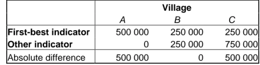
Table 2 - Allocation of transfer pool for villages A, B and C, $ (example)

Village

A B C

First-best indicator 500 000 250 000 250 000

Other indicator 0 250 000 750 000

The TAD is simply the sum of the absolute differences calculated for every village in the sample. The method to calculate the SSQ is straightforward. In this case the TAD equals 1 000 000 $ which is a fairly poor performance. Indicators are ranked according to their respective TADs (and SSQs); from the smallest to the largest (the smallest being the best performing indicator).

Results

We report the TAD in the first and third column of table 3. The indicators are ranked according to their respective TADs in the second and fourth column. The ranks specified in parentheses are those computed when SSQ is used as goodness-of-fit measure.

As it was the case in Vaillancourt (2001), for a given indicator using maximum values as targets for equalisation rather than mean values yields better fit. This is due to the fact that when using maximum value as a target the need to correctly match transfers equal to zero is reduced. For any given indicator, the TAD reported when mean value was used ranged from 2 to 5 times the size of the maximum value TAD. For example, the TAD for the worst fitting indicator (distance from the nearest water source) when mean value is used is equal to 1 588 323 $ which is more than twice as large as the maximum value TAD, 708 419 $. The mean value TAD for the best fitting indicator (population) is roughly five times larger than the maximum value TAD. Furthermore, our results show that the worst fitting indicator when maximum value is used (distance from the nearest water source) still outperforms the best fitting indicator with mean value (percentage of poor households) as a target for equalisation. This suggests that for any given indicator maximum value as a target for IET is preferable to mean value.

Population constitutes the best performing indicator when using maximum value as a target posting a TAD of 148 818$. It places fifth using the mean value method. This is of interest since many countries already use such an indicator. Thus, the data is usually readily available at the micro level and by age brackets. Correcting for age distribution

could improve the fit (data on age distribution was not available). Further studies are needed to verify its effectiveness.

Table 3 - Total absolute difference (TAD) and Total Sum of Squared Deviations

(SSQ) using maximum and mean value as targets, rank for fifteen indicators (in rupees) Indicator Max (R’s) Rank (SSQ) Mean (R’s) Rank (SSQ) %literate 291 763 5 (5) 1 024 608 9 (8) %poor 387 188 10 (8) 819 563 1 (1) %pucca 452 297 13 (14) 1 048 361 11 (12) %radio 398 776 12 (10) 979 149 6 (5) %tv 259 298 4 (4) 1 002 148 7 (7) %wall clock 301 797 6 (6) 1 026 546 10 (11) %iron box 312 085 7 (7) 844 004 2 (4) %land 363 639 8 (9) 933 214 3 (9) %sheep/goat 393 041 11 (12) 1 493 102 14 (14) % with water 244 441 3 (3) 1 019 741 8 (6) %child sick 516 495 14 (13) 1 270 263 13 (13) distance 708 419 15 (15) 1 588 323 15 (15) revenues 184 267 2 (2) 940 513 4 (3) lagged revenues 380 441 9 (11) 1 087 696 12 (10) per capita 148 818 1 (1) 953 164 5 (2)

Source: Tables A-3 and A-4

Average revenue collections per capita constitute the second best performing indicator when using maximum value as a target posting a TAD of 184 267 $. It places fourth using the mean value method. Martinez-Vasquez & Boex found similar results as it ranked first. However, as we have already mentioned this indicator does not have an efficient incentives structure. Thus, although effective in theory its use is discouraged in practice.

Overall, indicators of rurality perform fairly well. The percentage of households with a water connection is the third best performing indicator posting a TAD of 244 441$. It places eighth when using mean value as a target. Vaillancourt found similar results whereas Martinez-Vasquez & Boex found it to be the worst performing indicator. As opposed to average revenues per capita, this indicator satisfies the incentives constraint. Moreover, the data needed for its calculation is fairly easy to collect. Water connections are easier to account for than television sets for example because they cannot be easily disposed of or hidden7. Thus, this indicator satisfies the necessary incentives and ease of collection criterions while performing well. Developing countries looking for methods that are not data-intensive should pay attention to such an indicator.

The percentage of households who own a television set performed well posting a TAD of 259 298 $. None of the prior studies have examined this indicator. However as we have mentioned already, television sets are relatively easy to hide and thus would probably not yield efficient IETs in practice.

Lastly, using the SSQ method did not yield significant changes in the ranking of the indicators.

Conclusion

This section of the paper aimed to replicate two prior studies where imperfect indicators were used to simulate IETs. Fifteen indicators were computed and compared with a first-best measure of fiscal capacity. The performance of each indicator was established using total absolute difference (TAD) from the first-best equalisation transfer entitlement. As it was the case for Vaillancourt (2001), we find that for a given indicator using maximum values as targets for IET rather than mean values yields better fit. This is due to the fact that the need to match transfers equal to zero is reduced. Furthermore, our results show that the worst fitting indicator when maximum value is used still

7

If satellite dishes are used, this may be less of an issue as the need for a clear line of sight makes them hard to hide.

outperforms the best fitting indicator with mean value as a target for equalisation. This suggests that maximum value as a target for equalisation is always preferable to mean value. Second, population constitutes the best performing indicator when using maximum value as a target. Third, as it was the case for Boex & Martinez-Vasquez average revenue collections per capita perform well. However, this indicator does not have an efficient incentives structure. Finally, the percentage of households with a water connection is the third best performing indicator and it also satisfies the necessary incentives and ease of collection criterions. Vaillancourt also found this indicator to be effective. As a result, developing countries looking to devise IET schemes that are not data-intensive should pay attention to such an indicator. However, further studies are needed to clearly confirm its effectiveness.

3. An IET scheme for Kosovo

Introduction

The purpose of the second part of this paper is to design an IET scheme for Kosovo. Since the end of the tragic events that took place in the late 1990’s Kosovo has been ruled by a bifurcated central government comprised of the UNMIK (United Nations Mission in Kosovo) and of the PISG (Provisional Institutions of Self Government) with an assembly, a president and a ministerial council. However, due to limited data

availability the country still lacks a proper IET scheme. Using methods which were tested in the first part of this paper, four schemes will be devised. We will report and discuss differences in per capita allocations for a selection of municipalities.

Data

The data on tax assessment and other demographic characteristics was obtained as a by-product from work by François Vaillancourt on Kosovo Decentralisation for the UNDP8. Although data on tax assessment was available for 2004, 2005 and 2006 we only used 2005. Data on actual grants received came from the 2006 Kosovo Budget. Finally, data on majority and minority profiles was provided by the Statistical Office of Kosovo but was only available for 1991. From the 30 municipalities in the original dataset only 27 remain due to missing data. The municipalities that were excluded are Leposaviç, Zveçan and Zubin-Potok; these are Serbian municipalities that do not provide data to the relevant central agencies . The municipality of Fushe Kosove was also excluded because it is a significant outlier with respect to fiscal capacity. Indeed the municipality posts a 26.34 Euros tax assessment per capita which lies at roughly four standard deviations from a mean of 5.77. Thus, the final sample is comprised of 26 municipalities; the data re found in table A-5.

8

Data compiled by Luan Bicaj from multiple public sources such as Association of Kosovo

Municipalities 2005 and Organisation for Security and Co-operation in Europe Municipal Profiles 2005 and provided by François Vaillancourt..,.

The population data used to perform this analysis was derived from information on population figures available to the UNMIK Department of Local Administration (DLA) and the Central Fiscal Authority (CFA) as of the 8th of August 2001. The last valid Census was conducted in 1981; the Albanian majority boycotted the 1991 Census. The population of Kosovo adds up to a little more than 2 million people and is composed of 85-90% Albanians, 5-8% Serbs and other small minorities such as Romas, Turks, etc.

The 2001 population data is often contested by municipalities who claim that their population has now increased. This is probably true; however the important issue is the relative population size since the absolute size of the population does not affect the allocation of grants. So, “in this respect, it is plausible that internal migration since 2001 will have increased the population share of municipalities with greater economic activity such as Prishtine or Prizen. This means that using the 2001 population implicitly

equalises for fiscal potential since Prishtine which has greater local tax potential than poorer municipalities receives less per capita than it should while the others receive more.”9.

Methodology

The municipalities of Kosovo constitute sub-national government (SNGs) bodies which were the focus point of the first part of this paper. In 2006, the main source of municipal revenues is central government grants, which represent 79.6 % of total revenues with municipal own source revenues (MOSR) making up 20.4 %.

The actual setting of transfers to SNGs as a share of Kosovo generated revenues began in 2001-2002. This share of forecast central budget revenues was established at around 22% for 2005. This proportion is historically related to the needs of the

municipalities. It is divided into four specific grants:

9

The Education Grant: The amount of this grant awarded to the 26 municipalities studied

here was 73 132 291 Euros in 200510.

The Health Grant: The amount of this grant was 17 184 438 Euros for the 26

municipalitie) in 2005.

Additionally, there is a General Grant of 36 365 264 Euros for the 26 municipalities and a Property Tax Collection Incentive Grant.

This part of the paper will consider the sum of the Education, Health and General Grants which constitutes a total transfer pool of 125 681 993 Euros (excluding the Property Tax Grant).

Current Methods11

The allocation of the Education Grant uses a formula developed by the World Bank which allocates transfers to majority and minority populations on the basis of pupil/teacher ratios and a variety of other factors12. As for the allocation of the Health Grant it is based solely on the 2001 population data. Finally, the General Grant is the difference between the sum of these previous grants and the total transfer pool which is set at 22% of forecast central government revenue. The General Grant is comprised of two parts, a fixed amount of 100,000 Euros per municipality and the remainder divided according to the 2001 population data.

Revised Methods

To compute the revised methods we will make use of both shares and deviations. Using shares to simulate transfers is straightforward. For example, a municipality with a relatively greater population size would receive a proportional transfers – a larger slice of the pie. Using deviations requires a different approach which was laid out in the first part of the paper.

10

This in a sense assumes that the formula applied to the 30 municipalities would yield this amount for the 26;thsis debatable but is the simplest assumption that can be used here.

11

See Vaillancourt (2006) 12

First, we simulate a scheme based solely on population. Formally, 1) 1 1.00 i i n i i Pop Grant TP Pop = ⎛ ⎞ ⎜ ⎟ ⎜ ⎟ = ⋅ ⋅ ⎜ ⎟ ⎜ ⎟ ⎝

∑

where Granti is the total grant to municipality i, TP stands for transfer pool (125 681 993 Euros in our case), Popi represents the total population of municipality.

This and the current Kosovar scheme ignore fiscal capacity. Thus we propose an IET scheme based on Germany’s revenue sharing formula13 which accounts for differences in fiscal capacity. In this case 75 percent of the transfer pool is distributed on a per capita basis. The remaining 25 percent is allocated to municipalities with below-average fiscal capacity. For the purpose of our analysis, tax assessment per capita is used as a proxy for fiscal capacity. Formally,

2) 1 1 0.75 i 0.25 i i i n n i i i i i

Pop DevCap PopShare

Grant TP TP

Pop DevCap PopShare

= = ⎛ ⎞ ⎛ ⎞ ⎜ ⎟ ⎜ _× ⎟ ⎜ ⎟ ⎜ ⎟ = ⋅ ⋅ + ⋅ ⋅ ⎜ ⎟ ⎜ _× ⎟ ⎜ ⎟ ⎜ ⎟ ⎝

∑

∑

DevCapi is the deviation from the average tax assessment per capita PopSharei is the share of the total population for municipality i. This method is the same as in the first part of this paper. Remember that deviations for villages with above-average fiscal capacity are set to zero. The German approach was chosen because it has been shown to be significantly equalising14,15 while having minimal data requirements.

Third we use population, land area and number of villages to allocate the transfer pool. Formally,

13

See Ma (1997) pp. 12-14 14

See Vaillancourt & Bird (2004) p.15 15

3) 1 1 1 0.75 i 0.125 i 0.125 i i n n n i i i i i i Pop LA NbVil Grant Pop LA NbVil = = = ⎛ ⎞ ⎛ ⎞ ⎛ ⎞ ⎜ ⎟ ⎜ ⎟ ⎜ ⎟ ⎜ ⎟ ⎜ ⎟ ⎜ ⎟ = + + ⎜ ⎟ ⎜ ⎟ ⎜ ⎟ ⎜ ⎟ ⎜ ⎟ ⎜ ⎟ ⎝

∑

∑

∑

where LAi is land area and NbVili is the number of villages in municipality i. The fact that the percentages attributed to population are the same in method 2 and 3 will enable us to better compare the allocation of the transfer pool. The main advantage of this method is that the data needed for its computation can be easily obtained. Moreover, it requires minimal monitoring by the central government of data collection carried out by SNGs.

Fourth we compute an IET scheme which accounts for population, fiscal capacity and fiscal needs.

4) 1 1 1 1 0.50 i 0.125 i 0.125 i 0.25 i i i n n n n i i i i i i i i i

Pop LA NbVil DevCap PopShare

Grant

Pop LA NbVil DevCap PopShare

= = = = ⎛ ⎞ ⎛ ⎞ ⎛ ⎞ ⎛ ⎞ ⎜ ⎟ ⎜ ⎟ ⎜ ⎟ ⎜ _× ⎟ ⎜ ⎟ ⎜ ⎟ ⎜ ⎟ ⎜ ⎟ = + + + ⎜ ⎟ ⎜ ⎟ ⎜ ⎟ ⎜ _× ⎟ ⎜ ⎟ ⎜ ⎟ ⎜ ⎟ ⎜ ⎟ ⎝

∑

∑

∑

∑

Results

Our first method sees the transfer pool allocated using only population16. It yields three clear-cut winners, Podujevë, Prishtinë and Prizren respectively posting 7.68 €, 13.76 € and 7.41€ per capita increases in grants. These municipalities are also the most populous in Kosovo. Novobërde and Shtërpcë post the greatest decreases with 73.58 € and 58.63 € per capita. The total absolute difference (TAD) from the current Kosovar scheme is roughly 16 million Euros.

The second method allocates 75 percent of the transfer pool on a per capita basis. The remaining 25 percent is distributed using tax assessment per capita as a proxy for

16

fiscal capacity. This formula yields four winners Ferizaj, Malishevë, Podujeve and Skenderaj. Each of these municipalities post increases of more than 28 € per capita. Prizren and Prishtinë now post decreases of 3.87€, 0.85€ per capita while Novobërde and Shtërpcë post decreases of 9.06€ and 65.23€ respectively. This method yields a TAD of about 32 million Euros.

The third method utilises 75 percent population, 12.5 percent land area and 12.5 percent number of villages as equalisation factors. Prishtinë and Prizren post increases and Novobërdë and Shtërpcë post decreases smaller than those in methods 1 and 2. The TAD for this method is approximately 11 million Euros.

Finally, our fourth method is a variation on the third. It includes equalisation in terms of population, fiscal capacity and fiscal needs. For the first time Prishtinë posts a significant decrease whereas Novobërdë posts an increase.

First, we notice that methods that account for differences in fiscal capacity report decreases in per capita transfers to Prishtinë and Prizren. Indeed, the tax assessment per capita data suggest that the current scheme gives too high transfers to these municipalities. Second, methods 1 to 3 decreased transfers to Novobërdë and Shtërpcë. This may be evidence that the current scheme overestimates transfers to these municipalities as well.

Of all the methods reviewed in this analysis, the fourth is recommended because it accounts for both fiscal capacity and fiscal needs. Moreover, it is easy to compute and the necessary data is fairly easy collect.

Conclusion

In the second part of this paper we proposed four IET schemes for Kosovo. The fourth method is recommended because it accounts for both fiscal capacity and fiscal needs. Three out of the four formulas decreased transfers to Novobërdë and Shtërpcë. We also notice that methods accounting for differences in fiscal capacity report decreases in per capita transfers to Prishtinë and Prizren This consistency suggest than the current Kosovar scheme overestimates the needs of these municipalities. However, it is important to remember that our methods did not completely account for fiscal needs differentials. This fact could explain some unexpected results such as the negative correlation between a municipality’s share of total minority population and its average per capita grant. A new census is planned for late 2006 or 2007. This fresh data will enable us to better assess the fiscal capacity and fiscal needs of Kosovar municipalities and to design an optimal IET scheme which would account for fiscal gap differentials.

Table A-1 Intergovernmental Equalisation Transfers in Six Countries Country Number of Regions Number of equalisation programs Distributive pool Fiscal capacity categories Expenditures differential categories Fiscal effort

Australia 8 1 Federal VAT 18 (RTS) 41 No

Germany 16 3 Federal VAT 3 (RTS) - No

Horizontal Sharing 3(RTS) 2

Supplementary federal grants

from general revenue Variable -

Switzerland 26 3

Federal conditional grants from general revenue

3 (RTS and

macro) 2 Yes

FDT, withholding tax custom duties (petrol and motor fuel)

and National Bank's benefit 3 2

Cantonal contributions to social

security 3 2

China 31 9 Gap-filling (general revenue) - - No

Determined ad hoc by the

central government 13 (RTS) 12 Central VAT 13 (RTS) 12 General revenue - 1 (number of civil servants) Other programs

India 35 3 Total central taxes

2 (RTS and macro) plus

gap filling 2 Yes

General revenue 2 2

Specific purpose grants

Brazil 27 2

Federal personal and corporate

income tax and VAT No

For states - 2

For cities - 1

Table A-2 Final Dataset, 29 villages, Karnataka state, India.

Village ID 211111 211121 211131 211141 211151 211211 211221

Income mean 37428 14045 31031 21624 106453 30919 22763,75

Literacy rate %literate 0,4375 0,3125 0,5 0,5 0,375 0,8 0,5625

Poverty % poor 0,625 0,8125 0,6875 0,625 0,5625 0,625 0,6875 Type of house owned %pucca 0 0 0 0,125 0,375 0,25 0,0625

Asset ownership %radio 0,3125 0,1875 0,25 0,5 0,5 0,4375 0,4375 %tv 0,3125 0,125 0 0,3125 0,5625 0,3125 0,4375 %wall clock 0,5625 0,4375 0,625 0,625 0,8125 0,75 0,5625 %iron box 0,0625 0,0625 0,0625 0,1875 0,3125 0,3125 0,0625 %land 0,5 0,5 0,5625 0,9375 0,8125 0,9375 0,4375 %sheep/goat 0,125 0,25 0,25 0,125 0,0625 0 0,0625

Water connection %yes 0,25 0,25 0,25 0,25 0,25 0,375 0,25 Child 36 months

or less fell sick %no 0,75 0,875 0,6875 0,6875 0,9375 0,9375 0,8125 Distance from

source of water mean (mtr) 102 33 215 314 9 188 51

Total population 20000 9847 6436 7241 5330 3281 10024 Total revenues for SNG 2000-2001 1274827229141 213716 218551 204304 307170 1479770 1999-2000 906455 252766 271914 495796 204257 204927 481393

Table A-2 continued

Village ID 211231 211241 211251 211311 211321 211331 211341

Income mean 27654 54131 33738 34801 40213 25398 41350

Literacy rate %literate 0,5 0,75 0,5 0,5625 0,875 0,375 0,5625

Poverty % poor 0,5 0,4375 0,5625 0,625 0,625 0,8125 0,375 Type of house owned %pucca 0,25 0,375 0,4375 0 0,375 0 0,375

Asset ownership %radio 0,4375 0,5625 0,5 0,3125 0,4375 0,125 0,625 %tv 0,4375 0,4375 0,5625 0,4375 0,4375 0,25 0,75 %wall clock 0,625 0,6875 0,75 0,6875 0,6875 0,6875 0,9375 %iron box 0,0625 0,0625 0,375 0,4375 0,375 0 0,625 %land 0,5 0,625 0,125 0,4375 0,875 0,5625 0,625 %sheep/goat 0,125 0,0625 0 0,125 0,0625 0,0625 0

Water connection %yes 0,4375 0,25 0,25 0,25 0,25 0,375 0,25 Child 36 months

or less fell sick %no 0,75 0,9375 1 0,75 0,9375 0,8125 0,625 Distance from

source of water mean (mtr) 16 24 28 112 67 58 23

Total population 10500 8227 8164 12258 6516 9314 7701 Total revenues for SNG 2000-2001 598930 475323 482823 919288 643097 568524 279487 1999-2000 454130 558849 581608 594437 462455 961057 159273

Table A-2 continued

Village ID 211351 211362 215121 215131 215141 215151 215162

Income mean 58050 39900 25754 42041 29805 29802 35596

Literacy rate %literate 0,75 0,5 0,4375 0,6875 0,375 0,375 0,375

Poverty % poor 0,4375 0,625 0,8125 0,75 0,625 0,5625 0,6875 Type of house owned %pucca 0,1875 0,125 0,375 0,3125 0,4375 0,1875 0,1875

Asset ownership %radio 0,625 0,3125 0,3125 0,4375 0,125 0,25 0,3125 %tv 0,5 0,375 0,25 0,25 0,1875 0,0625 0,1875 %wall clock 0,875 0,25 0,5 0,8125 0,3125 0,5625 0,5 %iron box 0,5 0,25 0,125 0,3125 0,125 0,125 0,125 %land 0,8125 0,8125 0,4375 0,5625 0,875 0,625 0,625 %sheep/goat 0 0,0625 0,0625 0 0,0625 0,1875 0,0625

Water connection %yes 0,5625 0,5 0,25 0,25 0,3125 0,25 0,25 Child 36 months

or less fell sick %no 0,875 1 0,625 0,9375 1 0,9375 0,9375 Distance from

source of water mean (mtr) 177,13 160,19 72,813 81,688 95,813 32,375 229,75

Total population 5820 4983 5392 5281 3703 6438 3842 Total revenues for SNG 2000-2001 471519 371118 220271 357927 374989 427992 336447 1999-2000 229991 409641 218973 298837 299653 425531 254091

Table A-2 continued

Village ID 215231 215262 215321 215331 215341 215351 215362

Income mean 32213 23584 44509 56069 46569 34278 54206

Literacy rate %literate 0,5 0,375 0,5625 0,2 0,625 0,2667 0,625

Poverty % poor 0,5 0,8125 0,6875 0,6875 0,375 0,5 0,4375 Type of house owned %pucca 0,1875 0,25 0,3125 0,25 0,1875 0,125 0,125

Asset ownership %radio 0,375 0,125 0,3125 0,3125 0,375 0,375 0,5 %tv 0,3125 0,3125 0,375 0,4375 0,3125 0,1875 0,375 %wall clock 0,625 0,5625 0,75 0,8125 0,75 0,625 0,5 %iron box 0,3125 0,125 0,125 0,125 0,3125 0,0625 0,4375 %land 0,8125 0,4375 0,6875 0,625 0,875 0,75 1 %sheep/goat 0 0,0625 0,125 0,125 0,0625 0,0625 0,0625 Water connection %yes 0,25 0,1875 0,25 0,25 0,3125 0,25 0,3125 Child 36 months

or less fell sick %no 0,8125 0,875 0,75 0,75 0,75 0,875 0,75 Distance from

source of water mean (mtr) 80,625 85,625 72,75 30,125 37,375 28,938 32,9375

Total population 5694 7172 5000 5598 5363 6834 5400 Total revenues for SNG 2000-2001 2617881 688726 395655 443469 289620 539000 237002 1999-2000 442737 509477 361209 540782 344283 129000 284344 Source :Compilation by the author

Table A-3 Allocation of transfer pool (1 000 000 R’s) in rupees for fifteen indicators using maximum value as a target for equalisation, 29 villages, Karnataka state, India.

average

income %literate %poor %pucca %radio %tv

%wall

clock %iron box

Village 1 96 841 115 018 103 053 166 085 118 662 106 247 122 010 130 758 Village 2 63 832 72 809 88 792 81 772 81 793 74 730 80 095 64 379 Village 3 34 051 31 725 41 453 53 446 45 823 58 612 32 719 42 078 Village 4 43 089 35 693 37 310 42 951 17 185 38 467 36 811 36 821 Village 5 0 35 031 20 598 6 323 12 649 12 135 10 839 19 359 Village 6 17 385 3 235 16 906 11 677 11 680 17 430 10 008 11 917 Village 7 58 848 41 176 64 563 71 350 35 684 38 037 61 151 65 536 Village 8 58 041 51 758 27 051 37 369 37 379 39 843 53 379 68 648 Village 9 30 196 13 518 10 598 9 760 9 762 31 218 33 459 53 787 Village 10 41 644 40 243 31 550 0 19 375 18 587 24 902 23 722 Village 11 15 237 11 103 13 928 16 033 12 830 14 359 16 490 7 854 Village 12 61 613 50 353 63 161 101 793 72 728 46 514 49 853 26 714 Village 13 30 278 0 33 575 7 730 23 196 24 725 26 501 18 934 Village 14 52 959 61 216 83 986 77 346 88 418 56 548 37 880 67 660 Village 15 35 170 31 634 0 9 136 0 0 0 0 Village 16 19 761 9 563 7 497 27 618 0 17 667 5 917 8 456 Village 17 23 264 24 563 25 676 29 557 29 565 22 690 55 731 21 719 Village 18 30 524 31 009 48 620 6 397 31 991 32 736 38 376 31 335 Village 19 23 862 13 016 40 817 12 530 18 800 32 062 10 739 19 181 Village 20 19 910 24 338 19 080 0 35 152 25 292 37 650 21 520 Village 21 34 617 42 314 24 880 30 550 45 837 53 744 39 275 37 414 Village 22 19 097 25 251 24 746 18 231 22 795 26 242 27 344 22 328 Village 23 29 654 28 068 14 670 27 020 27 026 30 249 28 947 20 682 Village 24 41 692 47 138 64 671 25 525 68 084 38 100 43 753 41 680 Village 25 21 727 20 539 32 204 11 863 29 666 22 767 15 251 29 057 Village 26 19 786 49 670 36 056 19 923 33 214 21 242 11 384 32 533 Village 27 22 529 17 624 0 25 449 25 455 28 490 16 358 19 479 Village 28 34 601 54 648 17 607 40 537 32 437 46 677 34 742 44 680 Village 29 19 791 17 746 6 956 32 031 12 816 24 589 38 433 11 768 TAD 0 291 763 387 188 452 297 398 776 259 298 301 797 312 085 Rank 5 10 13 12 4 6 7

Table A-3 continued

%land %sheep/goat

% with water

%child

sick distance revenues

lagged revenues population Village 1 127 080 75 685 110 218 134 909 125 523 101 811 120 357 98 009 Village 2 62 568 0 54 266 33 211 15 482 55 249 79 385 48 255 Village 3 35 782 0 35 468 54 267 89 948 35 289 40 788 31 539 Village 4 5 751 27 402 39 904 61 055 149 998 39 984 26 143 35 484 Village 5 12 700 30 255 29 373 8 988 0 28 874 35 956 26 120 Village 6 2 606 24 832 10 849 5 533 39 846 15 442 13 897 16 078 Village 7 71 654 56 900 55 241 50 712 28 581 40 220 57 507 49 122 Village 8 66 717 39 734 23 146 70 827 4 551 54 355 65 450 51 455 Village 9 39 206 46 699 45 338 13 874 8 320 42 511 30 166 40 316 Village 10 90 779 61 789 44 991 0 10 199 42 042 27 123 40 007 Village 11 8 587 20 458 14 896 27 349 1 149 11 369 18 282 13 246 Village 12 87 623 46 387 67 553 82 685 85 111 60 627 69 724 60 070 Village 13 10 351 36 987 35 909 10 988 25 584 30 242 21 830 31 931 Village 14 51 783 52 870 30 797 47 120 30 831 47 737 0 45 643 Village 15 36 699 58 285 42 439 77 920 6 970 41 920 66 079 37 739 Village 16 13 868 44 049 0 19 629 66 352 28 335 38 538 28 521 Village 17 11 873 28 285 5 492 0 51 072 24 679 10 871 24 419 Village 18 38 543 30 607 29 715 54 557 23 233 29 035 35 091 26 423 Village 19 29 361 39 969 29 103 8 906 25 941 26 609 25 593 25 879 Village 20 5 882 21 020 16 325 0 21 746 17 064 8 574 18 146 Village 21 30 680 12 181 35 479 10 857 10 040 32 546 24 833 31 549 Village 22 18 309 21 809 21 173 6 479 57 548 18 381 14 804 18 828 Village 23 13 567 43 095 31 379 28 806 27 558 0 15 059 27 903 Village 24 51 267 40 711 47 429 24 189 37 150 33 533 23 979 35 146 Village 25 19 856 18 921 27 554 33 727 21 522 24 464 16 091 24 502 Village 26 26 677 21 184 30 850 37 761 7 874 27 383 3 832 27 433 Village 27 8 519 30 442 23 644 36 176 10 187 27 972 21 747 26 281 Village 28 21 712 38 792 37 661 23 049 9 060 33 460 59 923 33 490 Village 29 0 30 652 23 807 36 425 8 628 28 867 28 378 26 463 TAD 363 639 393 041 244 441 516 495 708 419 184 267 380 441 148818,094 Rank 8 10 3 14 15 2 9 1

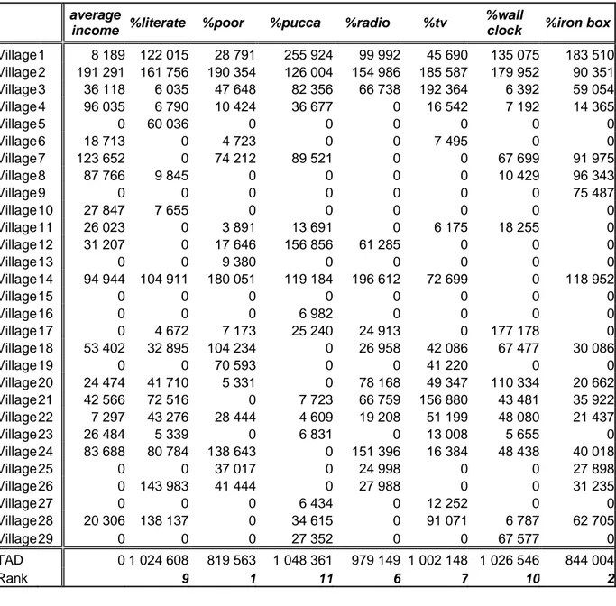
Table A-4 Allocation of transfer pool (1 000 000 R’s) in rupees for fifteen indicators using mean value as a target for equalisation 29 villages ,Karnataka state, India

average

income %literate %poor %pucca %radio %tv

%wall

clock %iron box

Village 1 8 189 122 015 28 791 255 924 99 992 45 690 135 075 183 510 Village 2 191 291 161 756 190 354 126 004 154 986 185 587 179 952 90 351 Village 3 36 118 6 035 47 648 82 356 66 738 192 364 6 392 59 054 Village 4 96 035 6 790 10 424 36 677 0 16 542 7 192 14 365 Village 5 0 60 036 0 0 0 0 0 0 Village 6 18 713 0 4 723 0 0 7 495 0 0 Village 7 123 652 0 74 212 89 521 0 0 67 699 91 975 Village 8 87 766 9 845 0 0 0 0 10 429 96 343 Village 9 0 0 0 0 0 0 0 75 487 Village 10 27 847 7 655 0 0 0 0 0 0 Village 11 26 023 0 3 891 13 691 0 6 175 18 255 0 Village 12 31 207 0 17 646 156 856 61 285 0 0 0 Village 13 0 0 9 380 0 0 0 0 0 Village 14 94 944 104 911 180 051 119 184 196 612 72 699 0 118 952 Village 15 0 0 0 0 0 0 0 0 Village 16 0 0 0 6 982 0 0 0 0 Village 17 0 4 672 7 173 25 240 24 913 0 177 178 0 Village 18 53 402 32 895 104 234 0 26 958 42 086 67 477 30 086 Village 19 0 0 70 593 0 0 41 220 0 0 Village 20 24 474 41 710 5 331 0 78 168 49 347 110 334 20 662 Village 21 42 566 72 516 0 7 723 66 759 156 880 43 481 35 922 Village 22 7 297 43 276 28 444 4 609 19 208 51 199 48 080 21 437 Village 23 26 484 5 339 0 6 831 0 13 008 5 655 0 Village 24 83 688 80 784 138 643 0 151 396 16 384 48 438 40 018 Village 25 0 0 37 017 0 24 998 0 0 27 898 Village 26 0 143 983 41 444 0 27 988 0 0 31 235 Village 27 0 0 0 6 434 0 12 252 0 0 Village 28 20 306 138 137 0 34 615 0 91 071 6 787 62 705 Village 29 0 0 0 27 352 0 0 67 577 0 TAD 0 1 024 608 819 563 1 048 361 979 149 1 002 148 1 026 546 844 004 Rank 9 1 11 6 7 10 2

Table A-4 continued

%land

% sheep/ goat

% with

water %child sick distance revenues

lagged revenues population Village 1 147 194 0 119 579 148 229 66 018 93 149 126 844 98 009 Village 2 72 471 0 58 875 0 0 140 403 159 837 48 255 Village 3 28 804 0 38 481 86 125 167 499 76 597 50 774 31 539 Village 4 0 0 43 294 96 898 332 475 91 371 0 35 484 Village 5 0 18 979 31 868 0 0 56 954 52 580 26 120 Village 6 0 60 083 0 0 67 655 0 0 16 078 Village 7 102 685 35 693 59 933 14 446 0 0 49 949 49 122 Village 8 77 277 0 0 77 820 0 65 593 77 543 51 455 Village 9 13 091 29 294 49 189 0 0 49 959 0 40 316 Village 10 201 364 149 502 48 812 0 0 46 934 0 40 007 Village 11 0 49 498 16 161 52 309 0 0 26 896 13 246 Village 12 125 570 0 73 290 90 850 64 598 24 366 58 183 60 070 Village 13 0 23 202 38 959 0 0 0 0 31 931 Village 14 41 685 33 165 0 13 423 0 49 349 0 45 643 Village 15 12 254 141 024 46 044 149 031 0 86 014 144 329 37 739 Village 16 0 106 578 0 0 107 236 3 254 53 914 28 521 Village 17 0 17 743 0 0 74 879 10 518 0 24 419 Village 18 55 235 19 200 32 239 104 347 0 54 392 46 982 26 423 Village 19 23 635 96 708 31 575 0 0 19 541 3 559 25 879 Village 20 0 13 185 0 0 7 811 0 0 18 146 Village 21 10 245 0 38 493 0 0 25 804 0 31 549 Village 22 6 114 13 680 22 971 0 111 361 0 0 18 828 Village 23 0 104 271 34 044 8 206 0 0 0 27 903 Village 24 73 469 25 538 111 968 0 468 0 0 35 146 Village 25 0 0 29 895 37 057 0 5 033 0 24 502 Village 26 8 908 0 33 470 41 489 0 5 518 0 27 433 Village 27 0 19 096 0 39 748 0 37 367 0 26 281 Village 28 0 24 334 40 860 0 0 7 302 134 291 33 490 Village 29 0 19 228 0 40 022 0 50 582 14 320 26 463 TAD 933 214 1 493 102 1 019 741 1 270 263 1 588 323 940 513 1 087 696 Rank 3 14 8 13 15 4 12 5

Table A-5 Original Dataset, 29 municipalities, Kosovo. MUNICIPALITY Total Tax Assessment 2005 Tax Assessment Per Capita Population Size in Square Km Density per Square Km Number of Villages %Majority DEÇAN € 204 877 € 4,10 50000 180 277,78 42 97,28% DRAGASH € 127 692 € 3,65 35000 434 80,65 37 57,78% FERIZAJ € 237 061 € 2,14 111000 345 322,01 44 88,10% FUSHE KOSOVE € 940 323 € 26,87 35000 96 364,58 15 56,63% GJAKOVË € 740 620 € 6,44 115000 521 220,73 84 92,85% GJILAN € 941 126 € 8,56 110000 515 213,59 63 76,54% GLLOGOVC € 167 834 € 2,80 60000 290 206,90 36 99,90% ISTOGU € 137 735 € 3,13 44000 454 96,92 51 76,68% KAMENICË € 231 078 € 4,20 55000 523 105,16 76 73,05% KAÇANIK € 156 438 € 3,64 43000 306 140,52 40 98,31% KLINA € 182 520 € 4,15 44000 308 142,86 54 82,75% LIPJAN € 293 734 € 3,92 75000 422 177,73 71 77,36% MALISHEVË € 111 513 € 2,14 52000 306 169,93 44 98,96% MITROVICA € 415 985 € 3,78 110000 350 314,29 44 78,98% NOVO BËRDË € 5 700 € 1,14 5000 92 54,35 15 40,03% OBILIQ € 181 718 € 6,99 26000 105 247,62 20 66,31% PEJA € 603 800 € 5,25 115000 603 190,71 97 75,46% PODUJEVE € 237 271 € 2,03 117000 602 194,35 78 97,91% PRISHTINE € 4 645 959 € 11,61 400000 854 468,38 48 77,63% PRIZREN € 884 205 € 4,02 220000 640 343,75 73 75,91% RAHOVEC € 217 939 € 3,46 63000 276 228,26 35 91,91% SHTËRPCË € 42 255 € 3,84 11000 248 44,35 16 33,83% SHTIME € 78 809 € 2,81 28000 134 208,96 22 92,38% SKENDERAJ € 110 263 € 1,97 56000 375 149,33 52 98,14% SUHAREKE € 260 744 € 3,26 80000 361 221,61 41 94,89% VITI € 286 406 € 5,62 51000 300 170,00 43 78,68% VUSHTRRI € 236 008 € 3,15 75000 344 218,02 66 88,48% Zvecan 16000 104 153,85 35 Leposavic 19000 536 35,45 72 Zubin Potok 15000 335 44,78 64 Total € 12 679 613 2236000 10959 5807 1478

Table A-6 Actual and revised grants using 100 percent population, 26 municipalities, Kosovo. (Method 1) Municipality Revised Grant Actual Grant Difference Difference Per Capita DEÇAN 2 921 478 2 992 808 -71 330 -1,43 DRAGASH 2 045 035 2 583 248 -538 213 -15,38 FERIZAJ 6 485 682 6 981 115 -495 433 -4,46 GJAKOVË 6 719 400 6 836 139 -116 739 -1,02 GJILAN 6 427 252 7 314 589 -887 337 -8,07 GLLOGOVC 3 505 774 3 988 124 -482 350 -8,04 ISTOG 2 570 901 2 814 898 -243 997 -5,55 KAMENICË 3 213 626 3 560 597 -346 971 -6,31 KAÇANIK 2 512 471 2 555 704 -43 233 -1,01 KLINË 2 570 901 2 917 054 -346 153 -7,87 LIPJAN 4 382 217 4 555 984 -173 767 -2,32 MALISHEVË 3 038 337 3 540 395 -502 058 -9,65 MITROVICA 6 427 252 7 346 002 -918 750 -8,35 NOVOBËRDË 292 148 660 028 -367 880 -73,58 OBILIQ 1 519 169 2 043 107 -523 938 -20,15 PEJË 6 719 400 6 773 239 -53 839 -0,47 PODUJEVE 6 836 259 5 937 433 898 826 7,68 PRISHTINE 23 371 826 17 867 639 5 504 187 13,76 PRIZREN 12 854 504 11 224 654 1 629 850 7,41 RAHOVEC 3 681 063 3 657 894 23 169 0,37 SHTËRPCË 642 725 1 287 614 -644 889 -58,63 SHTIME 1 636 028 1 746 391 -110 363 -3,94 SKENDERAJ 3 272 056 3 615 622 -343 566 -6,14 SUHAREKE 4 674 365 4 836 186 -161 821 -2,02 VITI 2 979 908 3 503 805 -523 897 -10,27 VUSHTRRI 4 382 217 4 541 724 -159 507 -2,13 Source :Calculations by the author

Table A-7 Actual and revised grants using 75 percent population and 25 percent tax assessment per capita. 26 municipalities, Kosovo. (Method 2)

Municipality Revised Grant Actual Grant Difference Difference Per Capita DEÇAN 2 254 241 2 992 808 -738 567 -14,77 DRAGASH 1 991 864 2 583 248 -591 384 -16,90 FERIZAJ 10 737 330 6 981 115 3 756 215 33,84 GJAKOVË 5 039 550 6 836 139 -1 796 589 -15,62 GJILAN 4 820 439 7 314 589 -2 494 150 -22,67 GLLOGOVC 4 759 005 3 988 124 770 881 12,85 ISTOG 3 104 083 2 814 898 289 185 6,57 KAMENICË 2 410 220 3 560 597 -1 150 377 -20,92 KAÇANIK 2 458 750 2 555 704 -96 954 -2,25 KLINË 1 925 071 2 917 054 -991 983 -22,55 LIPJAN 3 738 909 4 555 984 -817 075 -10,89 MALISHEVË 5 018 059 3 540 395 1 477 664 28,42 MITROVICA 5 874 013 7 346 002 -1 471 989 -13,38 NOVOBËRDË 614 726 660 028 -45 302 -9,06 OBILIQ 1 139 377 2 043 107 -903 730 -34,76 PEJË 5 039 550 6 773 239 -1 733 689 -15,08 PODUJEVE 11 649 543 5 937 433 5 712 110 48,82 PRISHTINE 17 528 869 17 867 639 -338 770 -0,85 PRIZREN 10 372 885 11 224 654 -851 769 -3,87 RAHOVEC 3 898 809 3 657 894 240 915 3,82 SHTËRPCË 570 118 1 287 614 -717 496 -65,23 SHTIME 2 208 062 1 746 391 461 671 16,49 SKENDERAJ 5 662 794 3 615 622 2 047 172 36,56 SUHAREKE 5 372 189 4 836 186 536 003 6,70 VITI 2 234 931 3 503 805 -1 268 874 -24,88 VUSHTRRI 5 258 606 4 541 724 716 882 9,56 Source :Calculations by the author

Table A-8 Actual and revised grants using 75 percent population, 12.5 percent land area and 12.5 percent for the number of villages. 26 municipalities, Kosovo. (Method 3)

Municipality Revised Grant Actual Grant Difference Difference Per Capita DEÇAN 2 987 809 2 992 808 -4 999 -0,10 DRAGASH 2 673 251 2 583 248 90 003 2,57 FERIZAJ 5 946 983 6 981 115 -1 034 132 -9,32 GJAKOVË 6 888 759 6 836 139 52 620 0,46 GJILAN 6 404 762 7 314 589 -909 827 -8,27 GLLOGOVC 3 527 849 3 988 124 -460 275 -7,67 ISTOG 3 269 662 2 814 898 454 764 10,34 KAMENICË 4 165 329 3 560 597 604 732 11,00 KAÇANIK 2 856 932 2 555 704 301 228 7,01 KLINË 3 074 167 2 917 054 157 113 3,57 LIPJAN 4 820 499 4 555 984 264 515 3,53 MALISHEVË 3 299 970 3 540 395 -240 425 -4,62 MITROVICA 5 911 566 7 346 002 -1 434 436 -13,04 NOVOBËRDË 547 681 660 028 -112 347 -22,47 OBILIQ 1 549 400 2 043 107 -493 707 -18,99 PEJË 7 177 121 6 773 239 403 882 3,51 PODUJEVE 7 032 143 5 937 433 1 094 710 9,36 PRISHTINE 19 469 424 17 867 639 1 601 785 4,00 PRIZREN 11 545 406 11 224 654 320 752 1,46 RAHOVEC 3 624 911 3 657 894 -32 983 -0,52 SHTËRPCË 1 070 637 1 287 614 -216 977 -19,73 SHTIME 1 707 441 1 746 391 -38 950 -1,39 SKENDERAJ 3 682 168 3 615 622 66 546 1,19 SUHAREKE 4 577 900 4 836 186 -258 286 -3,23 VITI 3 234 455 3 503 805 -269 350 -5,28 VUSHTRRI 4 635 769 4 541 724 94 045 1,25 Source :Calculations by the author

Table A-9 Actual and revised grants using 50 percent population, 12.5 percent land area, 12.5 percent for the number of villages and 25 percent fiscal capacity. 26 municipalities, Kosovo. (Method 4) Municipality Revised Grant Actual Grant Difference Difference Per Capita DEÇAN 2 320 572 2 992 808 -672 236 -13,44 DRAGASH 2 620 080 2 583 248 36 832 1,05 FERIZAJ 10 198 632 6 981 115 3 217 517 28,99 GJAKOVË 5 208 909 6 836 139 -1 627 230 -14,15 GJILAN 4 797 949 7 314 589 -2 516 640 -22,88 GLLOGOVC 4 781 079 3 988 124 792 955 13,22 ISTOG 3 802 845 2 814 898 987 947 22,45 KAMENICË 3 361 922 3 560 597 -198 675 -3,61 KAÇANIK 2 803 211 2 555 704 247 507 5,76 KLINË 2 428 337 2 917 054 -488 717 -11,11 LIPJAN 4 177 190 4 555 984 -378 794 -5,05 MALISHEVË 5 279 692 3 540 395 1 739 297 33,45 MITROVICA 5 358 327 7 346 002 -1 987 675 -18,07 NOVOBËRDË 870 259 660 028 210 231 42,05 OBILIQ 1 169 608 2 043 107 -873 499 -33,60 PEJË 5 497 271 6 773 239 -1 275 968 -11,10 PODUJEVE 11 845 427 5 937 433 5 907 994 50,50 PRISHTINE 13 626 467 17 867 639 -4 241 172 -10,60 PRIZREN 9 063 787 11 224 654 -2 160 867 -9,82 RAHOVEC 3 842 658 3 657 894 184 764 2,93 SHTËRPCË 998 030 1 287 614 -289 584 -26,33 SHTIME 2 279 475 1 746 391 533 084 19,04 SKENDERAJ 6 072 906 3 615 622 2 457 284 43,88 SUHAREKE 5 275 723 4 836 186 439 537 5,49 VITI 2 489 478 3 503 805 -1 014 327 -19,89 VUSHTRRI 5 512 157 4 541 724 970 433 12,94 Source :Calculations by the author

The Education Grant

The Education Grant uses a formula developed by the World Bank that was first applied in 2004, which allocates funding towards majority and minority populations on the basis of pupil/teacher ratios of 21.3 for majority pupils and 14.2 for minority pupils.

• The formula utilized is as follows:

o The number of minority and majority pupils in a municipality, - which should be obtained from official Directorate of Education reports to the MEST (Ministry of Education, Science and Technology), - are separately divided by the pupil/teacher ratio for that population type18. The resulting number of teachers is then multiplied times the Kosovo-wide average salary per teacher from payroll records.

ƒ Pupil/teacher ratios are set by the World Bank formula at 1 to 21.3 for majority pupils and 1 to 14.2 for minority pupils.

ƒ Formulae are:

No. Majority Teachers (NMAT) = No. Majority Pupils (NMAP) / 21.3 (Rounded Up) No. Minority Teachers (NMIT) = No. Minority Pupils (NMIP) / 14.2 (Rounded Up) Teacher Cost Need (TCN) = (NMAT+NMIT) x Kosovo-wide Average Salary of Teacher

o The number of administrative and support staff, as reported at thetimeof budget formulation, multiplied by the average salary per administrative and support employee from payroll records. This number, when added to the above, gives the total Wage Bill.

ƒ Formulae are:

Support Staff Cost Need (SSCN) = No. Admin & Support Staff 2004 x Kosovo-wide Average Salary of Staff

Wage Bill (WB) = TCN + SSCN = WB

o Good and Services: a fixed amount per school (500 Euro for each pre-primary and pre-primary school, 1,000 per secondary school) is added to a fixed amount per student differentiated by majority and minority students.

17

ƒ Fixed amounts per student for goods and services are set by the World Bank formula at €18 per Albanian student and €22.5 per student of other ethnic background.

ƒ The formula is:

Goods & Services (GS) = (NMAP x 18) + (NMIP x 22.5) = GS

o Capital Outlays: €5 per student is allocated to the municipality. ƒ The formula is:

Capital Outlays (CO) = (NMAP + NMIP) x 5 = CO o Master Formula Calculations:

Estimated Education Need (EEN) = WB + GS + CO = EEN

EEN / Combined Total of All Municipalities’ EEN = Percentage of Available Education Grant Funding to that municipality.

3. References

Bird, R. and Tarasov, A. (2002) “Closing the Gap: Fiscal Imbalances and

Intergovernmental Transfer in Developed Federations”, International Studies Program,

Andrew Young School of Policy Studies, Georgia State University, March.

Boadway, Robin and F. Flatters (1982) “Efficiency and Equalisation Payments in

Federal System of Governements, Canadian Journal of Economics 15, 613-633.

Boadway, Robin (2004) “The Theory and Practice of Equalisation”, Department of Economics, Queen’s University, WP#1016.

Boex, Jamie and Martinez-Vasquez, J.(2004),“Designing Intergovernmental

Equalisation Transfers with Imperfect Data : Concepts, Practices and Lessons” ,

Georgia State University.

Bernd Spahn, Paul. (2004) “Intergovernmental Transfers: The Funding Rule and

Mechanisms”, International Studies Program, Andrew Young School of Policy Studies,

Georgia State University, WP # 04-17.

Buchanan, James M. (1950) “Federalism and Fiscal Equity”, American Economic Review, # 40-4, 583-599.

Day, Kathleen and Winer, Stanley L. (2005) “Policy-Induced Internal Migration: An

Empirical Investigation of the Canadian Case”, CESifo, November, WP#1605.

Kehmani, Stuti (2004) “The Political Economy of Equalisation Transfers”, International Studies Program, Andrew Young School of Policy Studies, Georgia State University, WP # 04-13.

Ma, Jun (1997) “Intergovernmental Fiscal in Nine Countries: Lessons for Developing

Countries”, World Bank, Economic Development Institute, WP# 1822.

Rao, Govinda (2004), “Changing Contours in Fiscal Federalism in India”, International Symposium on Fiscal Decentralization in Asia Revisited, Hitotsubashi University, Tokyo, February.

Shah, Anwar (1994) “A Fiscal Needs Approach to Equalisation Transfers in

Decentralized Federations”, World Bank, Policy Research Department, Public

Economics Division, WP #1289.

Vaillancourt, François (2001), “Simulating Intergovernmental Equalisation Transfers

Vaillancourt, F. and Bird, R. (2004), “Expenditure-based equalisation transfers”, International Studies Program, Andrew Young School of Policy Studies, Georgia State University, November, WP # 04-10.

Vaillancourt, François (2006), “Fiscal Decentralisation in Kosovo”, prepared for UNDP, July.