HAL Id: hal-00909457
https://hal.archives-ouvertes.fr/hal-00909457
Submitted on 26 Nov 2013HAL is a multi-disciplinary open access archive for the deposit and dissemination of sci-entific research documents, whether they are pub-lished or not. The documents may come from teaching and research institutions in France or abroad, or from public or private research centers.
L’archive ouverte pluridisciplinaire HAL, est destinée au dépôt et à la diffusion de documents scientifiques de niveau recherche, publiés ou non, émanant des établissements d’enseignement et de recherche français ou étrangers, des laboratoires publics ou privés.
Modelling of the gravity compensators in robotic
manufacturing cells
Alexandr Klimchik, Yier Wu, Stéphane Caro, Claire Dumas, Benoît Furet,
Anatol Pashkevich
To cite this version:
Alexandr Klimchik, Yier Wu, Stéphane Caro, Claire Dumas, Benoît Furet, et al.. Modelling of the gravity compensators in robotic manufacturing cells. The IFAC Conference on Manufacturing Mod-eling, Management and Control (MIM 2013), Jun 2013, Saint Petersburg, Russia. pp.820-825. �hal-00909457�
A. Klimchik*, Y. Wu*, S. Caro**, C. Dumas***, B. Furet*** and A. Pashkevich*
*Ecole des Mines de Nantes, 4 rue Alfred-Kastler, Nantes 44307 France (Tel: +33-251-85-83-00; e-mail: [email protected], [email protected], [email protected]). **Centre National de la Recherche Scientifique, France (e-mail:[email protected]) *** University of Nantes, France, (e-mail: [email protected], [email protected])
Abstract: The paper deals with the modeling and identification of the gravity compensators used in heavy industrial robots. The main attention is paid to the geometrical parameters identification and calibration accuracy. To reduce impact of the measurement errors, the design of calibration experiments is used. The advantages of the developed technique are illustrated by experimental results .
Keywords: industrial robot, calibration, gravity compensator, geometrical modeling.
1. INTRODUCTION
Currently, aeronautic industry requires high-precision machining of huge aircraft component made from the high performance materials. For these applications, robots are quite attractive due to their large workspace that can be also easily extended. Another considerable advantage is their capability to process the parts with complex shape and geometry. However, processing of these materials causes essential cutting forces that are generated by tool-workpiece interaction during the material removal. Since these forces decrease the machining accuracy, the robot manufactures try to improve the robot stiffness by increasing the link cross-sections. This approach obviously leads to augmentation of robot link weights. So, the gravity forces applied to the manipulator components become non-negligible and also contribute to the position errors. To overcome this difficulty, the link weights are tended to be balanced by gravity compensators, which considerably complicate the stiffness modeling of these heavy manipulators.
The problem of stiffness modeling for the heavy manipulators with gravity compensators has been in the focus of rather limited number of works. In contrast, for conventional serial manipulators without gravity compensators, the problem has been studied by a number of authors that considered both industrial and medical robots with essential compliance in the links and joints (Meggiolaro 2005, Kövecses 2007). Relevant works are mainly based on the virtual joint method (VJM), which lumps the elastostatic properties of the robot components in virtual springs. To our knowledge, the stiffness modeling for the manipulators with gravity compensators has not been studied in detail yet. Currently, the main activity in this area focuses on the gravity compensator design (Takesue 2011, De Luca 2011). On the other hand, since the considered robots include closed loops induced by the compensators, some technique previously developed for the parallel manipulators can be adopted (Bouzgarrou 2004, Company 2005, Pashkevich 2011).
This paper focuses on the geometrical and stiffness modeling of the spring-based gravity compensators that can be integrated in a VJM-based stiffness model of a serial manipulator (Klimchik 2012). The main attention is paid to the identification of the model parameters and calibration experiment planning. The developed approach is confirmed by the experimental results that deal with the industrial robot employed in manufacturing of large-dimensional aircraft components.
To address these problems, the remainder of the paper is organized as follows. Section 2 presents the gravity compensator model. In Section 3, calibration methodology is presented. Section 4 proposes identification algorithms. Sections 5 is devoted to the experiment design. Experimental validation is presented in Section 6. Finally, Section 7 summarizes the main contributions.
2. GRAVITY COMPENSATOR MODEL
The mechanical structure of the gravity compensator under study is presented in Fig. 1. The compensator incorporates a passive spring attached to the first and second links, which creates a closed loop that generates the torque applied to the second joint of the manipulator. Corresponding model is presented in Fig. 2, where the most essential geometrical parameters are denoted as ax, y, and the compensator is
described by the spring compliance kc and the preloadi g
0
a L
n
s . This design allows us to limit the stiffness model modification by incorporating in it the compensator torque and adjusting the virtual joint stiffness matrix that here depends on the second joint variable q2 only.
The compensator geometrical model includes three node points P0, P1, P2, where two distances P P1, 2 , P P0, 2 are
constants and the third one P P0, 1 varies and depends on .
Let us denote them
2
q
1, 2
L P P , a P P1, 2 , s P1,P2 .
Besides, let us introduce the angles , and the distances
x
Using these notations, the variable s describing the compensator spring deflection can be computed from the expression 2 2 2 2 · · ·co 2 s( a L ) s a L q (1)
which defines the function s q
2 .0 P 2 P 1 P 01 P 02 P
Fig. 1. Gravity compensator of robot KUKA KR-270 TM
x a y a 2 q L 0 P P 1 P 2 a c k 2 q k s F c F l F O s
Fig. 2. Model of the gravity compensator
This mechanical design allows to balance the manipulator weight for any given configuration by adjusting the compensator spring preloading. It can be taken into account by introducing the zero-value of the compensator length s0
corresponding to the unloaded spring. Under this assumption, the compensator force applied to the node P1 can be
expressed as follows
0
·( )
s c s
F K s (2)
where kc is the compensator spring compliance.
Further, the angle between the compensator links P0P1 and
P1P2 (see Fig. 2) can be found from the expression
2
sina s·sin(q ) (3)
which allows us to compute the compensator torque Mc
applied to the second joint
0 ·(1 / )· · ·sin( c c s s L M K a q2) 2 q (4) Upon differentiation of the latter expression with respect to
2, the equivalent stiffness of the second joint (comprising
both the manipulator and compensator stiffnesses) can be expressed as: q 2 2 0 · · c K K K aL (5)
where the coefficient
2 2 0 2 2 2 sin cos co · ( ) ( ) s( q s a L q q s s q2) (6)
highly depends on the value of joint variable 2 and the initial preloading in the compensator spring described by
q
0
s . Hence, using expression (5), it is possible to extend the classical stiffness model of the serial manipulator
(F) 1 (F)T
1 C θ ( θ θθ) θ K J K H J (7)by modifying the virtual spring parameters in accordance with the compensator properties. Here, C θ are stiffness
matrices in the Cartesian and joint spaces respectively,
θ are corresponding Jacobian and Hessian matrices
(for more details see Klimchik 2012). While in the paper this approach has been used for the particular compensator type (spring-based, acting on the second joint), the similar idea can be evidently applied to other compensator types.
,
K K
(F) θ , θ
J H
Summarizing this Section, it is worth mentioning that the geometrical and elastostatic models of a heavy manipulator with a gravity compensator should include some additional parameters (ax, ay, L and Kc, s0 for the presented case)
that are usually not included in datasheets. For this reason, the following Sections focus on the identification of the extended set of manipulator parameters.
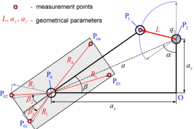
3. MODEL CALIBRATION METHODOLOGY In contrast to the serial manipulator that can be treated as a principal mechanism of the considered robots, geometrical data concerning gravity compensators are usually not included in the technical documentation provided by the robot manufacturers. For this reason, this Section focuses on the calibration methodology of the geometrical parameters for the described above compensator mechanism (see Fig. 1). The geometrical structure of the considered gravity compensator is presented in Fig. 2. Its principal geometrical parameters are denoted as L, ax, ay, where ax a·cos,
·sin
y
a a (see notation in Section III). As follows from the figure, the identification problem can be reduced to the determination of relative locations of points P0 and P1 with
respect to P2.
It is assumed that the measurement data are provided by the laser tracker whose "world" coordinate system is located at the intersection of the first and second actuated manipulator joints. The axes Y, Z of this system are aligned with the axes of joints #1 and #2 respectively, while the axis X is directed to ensure right-handed orthogonal basis. To obtain required data, there are several markers attached to the compensator mechanism (see Fig. 3). The first one is located at point P1,
which is easily accessible and perfectly visible (the center of the compensator axis P1 is exactly ticked on the fixing
locate the marker precisely. For this reason, several markers P0i are used that are shifted with respect to P0, but located on
the rigid component of the compensator mechanism (these markers are rotating around P0 while the joint coordinate 2
is actuated). It should be noted that for the adopted compensator geometrical model (which is in fact a planar one), the marker location relative to the plane XY is not significant, since the identification algorithm presented in the following sub-section will ignore Z-coordinate.
q
Using this setting, the identification problem is solved in two steps. The first step is devoted to the identification of the relative location of points P1 and P2. Here, for different
values of the manipulator joint coordinates {q2i, i1, }m , the laser tracker provides the set of the vectors
1ip describing the points that are located in an arc of the circle. After matching these points with a circle, one can obtain the desired value of (circle radius) and the Cartesian coordinates 2 of the point P2 (circle center) with respect to
the laser tracker coordinate system.
L p x a y a 2 q L 0 P 2 P 1 P a O 02 P 01 P 1 R 2 R 2 1 , x, y L a a 03 P 04 P 3 R 4 R
Fig. 3. Geometrical parameters of the gravity compensator and location of the measurement points labelled with markers The second step deals with the identification of the relative location of points P0 and P2. Relevant information is
extracted from two data sets
01i
p and that are provided by the laser tracker while targeting at the markers P01 and P02. Here, the points are matched to two circle arcs
with the same center (explicitly assuming that the compensator model is planar), which yields the Cartesian coordinates 0 of the point P0, also with respect to the laser
tracker coordinate system. Finally, the desired values
02 i p p x a , yare computed as a projection of the difference vector
2 on the corresponding axis of the coordinate
system.
a
0
a p p
As follows from the presented methodology, a key numerical problem in the presented approach is the matching of the experimental points with a circle arc. It looks like a classical problem, however, there is a particularity here caused by availability of additional data
q2i describing relativelocations of the points
. This feature allows us to reformulate the identification problem and to achieve higher accuracy compared with the traditional approach.
1
i
p
4. IDENTIFICATION ALGORITHMS
The above presented methodology requires solution of two identification problems. The first one aims at approximating of a given set of points (with additional arc angle argument) with an arc circle, which provides the circle center and the circle radius. The second problem deals with an approximation of several sets of points by corresponding number of circle arcs with the centers on the same rotation axis. Let us consider them sequentially.
4.1 Algorithm #1
To match the given set of points
with additional set ofangles
i
p
qi with a circle arc, let us define the affine mapping i ip R u t (8)
where denotes the set of reference points located on the unit circle whose distribution on the arc is similar to i,
[cos , sin , 0]T i qi qi
u
p is the scaling factor that defines the
desired circle radius, is the orthogonal rotation matrix, is the vector of the translation that defines the circle center. It worth mentioning that such a formulation has an advantage (in the sense of accuracy) comparing to a traditional circle approximation and it is a generalization of Procrustes problem known from the matrix analysis.
R t
Using equation (8), the identification can be reduced to the following optimization problem
1 min, , T i i i i i m F
p R u t p R u t R t (9) which should be solved subject to the orthogonality constraint R RT I. After differentiation with respect to t , the latter variable can be expressed as
1 1 1 1 i m i m m
t p R m i i
u (10)That leads to the simplification of (9) to
1 min, m i r T i i i i F
R p R u p R u (11) where 1 1 1 ; 1 i i i i m i i i i m m
p p p u u m u (12)Further, differentiation with respect to yields to
1 1 m T i i i i m i
p R u
u u T i (13)So, finally, after relevant substitutions the objective function can be presented as 1 1 1 1 2 min m m m i i i T T T i i i i i i F
p p
u u
p R u R (14)where the unknown matrix must satisfy the orthogonality constraint
R
T
R R I. Since the matrix is included in the second term only, the problem can be further simplified to
R
1 1 max m T m i i i i i i F
trace
R p Ru R u p T (15)and can be solved using SVD-decomposition of the matrix 1 m i i T i
u p UΣ V (16)where the matrices are orthogonal and is the diagonal matrix of the singular values. Further, using the same approach as for the Procrustes problem, it can be proved that the desired rotation matrix can be computed as
,
U V Σ
T
R V U (17)
which sequentially allows to find the scaling factor defining the arc radius and the vector defining the arc center.
t
4.2 Algorithm #2
The second problem aims at approximating of several point sets i by corresponding number of concentric circle arcs with the centers 0 on the rotation axis n. It should be noted that the data set
1 ,..., k i p p j p
qi is not useful here, sincethe required angles
are not measured directly and i cannot be computed without having exact compensator geometry. In this case, the objective function can be written in the straightforward way
0 2 2 0 0 1 1 minj, j k m j j j j j i i j i R T F
R p p p p p (18)where Rj denotes the j-th ark radius and 0
j
p is the corresponding center point. However, for this formulation it can be easily proved that the optimization problem (18) does not lead to a unique solution. In fact, it gives the rotation axis passing through the center points 0
j
p , which can be expressed as 0 c j j p p n (19)
where is the axis direction vector, pc is a point belonging
to the axis, and
n
j
are corresponding scalar factors.
To solve the problem (18), first the objective function F can be differentiate with respect to 2
j
R that yields the following expressions for the arc radii
2 1 0 1 m j j T j
0 j j i i i R m
p p p p min s (20) Further, after relevant substitution, the objective can berewritten as
1 1 2 2 k m j j i i T c j j i F
p n p (21) where 1 1 1 ; m m 1 j j j j j j i i l l i i i i i T T m s m
p p p p p p pj j l
(22)To solve the above mentioned ambiguity, additional objectives should be considered
2 min j j R R (23)
which leads to the following solution for the scalar parameter
1
1 T m i c i j j m p
p n (24)Further, after differentiation (21) with respect to pc
1 1
1 1 1 2 k m j j k m i i i i j i c j i T j j s
p p p
p (25)one can compute the point on the desired rotational axis as
1
1 1 1 1 2 k m k m 1 j j c j i i i j i T j j i i s
p p p p (26)The remaining unknown vector n can be obtained from the orthogonality constraints
pijp0j
Tn0, i1, ,m j k1,that leads to the following optimization problem
1 2 0 1 min k m j j T i j i f
n p p n (27)that after substitution in it (19), (24) and (26) gives
2 1 1 min k m j i j T i f
n p n (28)Further, differentiation (28) with respect to , the optimization problem reduces to the solving following homogeneous linear equation system
n 1 1 k m j j i i j i T
p p n 0 (29)Non-trivial solution of this system can be found using the singular value decomposition of the matrix k1 m1 j j
i i j i T
p p 1 1 k m j j i i j i T
p p UΣ VT (30) where the vector is the last column of the matrix n V.It should be mentioned that practical application of the latter expressions is essentially simplified by the adopted assumption concerning orientation of the reference coordinate system, where the direction of the rotation axis is close to Z-direction.
n
Hence, the developed algorithms allows us to identify the compensator geometrical parameters L, ax, y that are directly related to the above mentioned rotation center points P0, P2 and corresponding radii. Below they will be applied to
the processing of the experimental data.
a
5 DESIGN OF CALIBRATION EXPERIMENTS The main idea of the calibration experiment design is a set of robot configurations (as well as marker locations) that ensure the best identification accuracy. The key issue here is the ranging of different plans in accordance with the prescribed performance measure.
For the considered identification problem, the design variables are the set of angles
and the marker locations. The objective functions to be minimized are computed via the covariance matrix that describes the identification errors for the geometrical parameters and to be estimated. Since two identification algorithms are independent, selection of the optimal configurations
2iq
L a
q2iAssuming that each experiment includes the additive measurement errors in the Cartesian coordinates εi, expression (13) allows us to present the variance of the parameter in the following way
2 1 1 1 var iT T i T T m m m i i i i i i i E
u R ε
ε R u
u u (31)where denotes the expectation and the orthogonal matrix defines the orientation of the base coordinate system. Following usual assumption concerning the measurement errors (independent identically distributed, with zero expectation and standard deviation
(.) E
R
2
for each coordinate) that allows to present the covariance error matrix as
i iT2
E ε ε I, the above expression (31) reduces to
2
1 var T i i m i
u u (32)Further, it can be proved that
1 i m T i i m
u u q L . So, the variance (32) does not depend on the angles 2i. Thus, theidentification accuracy for the parameter depends on the number of experiments only.
For the remaining geometrical parameter a , the identification error depends on the estimation precision of relative location of the points P2 and P0. Since relevant
identification algorithms employ independent measurement data, the variance can be computed as the sum of the traces of cov 2 and cov 0 , where t1 and 2 are the
vectors of Cartesian coordinates for the points P2 and P0.
var a
( )t ( )t t
For the point P2, expression (10) leads to the following
covariance matrix
1 1 1 1 2 2 2 cov m T i m m m i i i i i i i m E
t ε ε R u u RT T
uis simplification is based on the
(33) which can be further simplified down to
1 2
2 1 2 1 cov T i m m i i i m m
t I u (34)Th above derived expressions
1
2 1 T i i m m i iE
ε ε m I and and on the assumption that z-axis of the coordinate system is directed along the second joint axis. Hence, for the point P2, theoptimization problem that is related to the design of calibration experiment, can be formulated as
2 2 / E m q
2 2 2 21cos 1sin 2 min
i i m i i m i q q F
(35)This problem should be solved taking into account joint limits of the industrial robot. In the case when the range of angles q2 is over , it is possible to achieve zero value of this objective since equations 1cos 2 0
m
i qi
and1
are solvable. It should be noted similar
equations arise in calibration experiment design for some robots without gravity compensators and have been studied in details in our previous work (Klimchik 2011).
2
sin q 0 m
i i
For the point P0, similar expression includes a set of the
angles that can be recomputed to the joint angles i requires for the manipulator control (see Fig. 3). Here, it is
reasonable to find optimal marker locations on the rigid part of the gravity compensator. It can be proven that using these assumptions, the design of experiment reduces to the following optimization problem
2i
q
1
2 2
1
cos sin min
j j j k k j j F
(36)where are the angles around the point Pj 0 between the
compensator spring and j-th marker location. It is clear that in this case the best solution is produced by similar equations
1
jcosj 0 k
and j1 , but contrary to (35), this problem can be easily solved by locating the markers on the opposite sides of the compensator rotation axis.sin j 0 k
Thus, the calibration experiment design that produces the sets of the optimal manipulator configurations and the marker locations described by the variables
q2i
and
jrespectively, is reduced to the solution of the above presented trigonometric equations that allows us essentially increase the calibration accuracy.
6 EXPERIMENTAL RESULTS
To demonstrate efficiency of the developed technique, the experimental study has been carried out. The experimental setup employed the robot KR-270 and the Leica laser tracker, which allowed us to measure the Cartesian coordinates of the markers attached to the compensator elements with the accuracy of 10 μm (see Figs 1, 3). Six different manipulator configurations where considered that differed in the value of the joint angle 2 and three markers has been used. The
experimental data are presented in Table 1.
q
These data has been processed using the developed identification algorithm presenting in the Section 4. The obtained values for the parameters of interest L, ax, y are
given in Table 2, which also includes the identification errors computed using the Gibbs sampling technique.
a
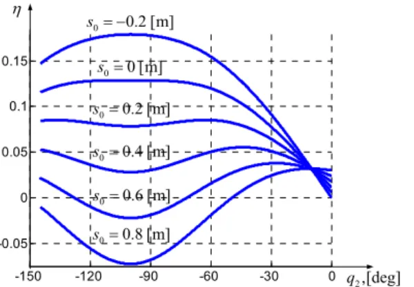
In addition, there were evaluated the elastostatic properties of the gravity compensator. Corresponding curves describing influence of the compensator on the equivalent stiffness of the manipulator joint (see eq. (6)), are presented in Fig. 4. They demonstrate essential non-linearity of the compensator impact throughout of the robot workspace, which, in addition, highly depend on the spring preloading s0.
Table 1. EXPERIMENTAL DATA
P1 P01 P02 q2 [deg] x, [mm] y, [mm] x, [mm] y, [mm] x, [mm] y, [mm] -0.01 -31.84 183.86 -872.10 -125.38 -813.50 -255.59 -30 -118.44 143.42 -872.30 -126.07 -813.33 -256.18 -60 -173.30 65.12 -872.50 -109.90 -825.09 -244.64 -90 -181.76 -30.14 -868.43 -78.20 -844.66 -219.04 -120 -141.45 -116.82 -858.90 -47.60 -859.43 -190.44 -145 -78.10 -165.47 -852.53 -33.68 -864.66 -176.01
Table 2. GEOMETRICAL PARAMETERS
L, [mm] ax, [mm] ay, [mm]
value 184.72 685.93 120.30
7. CONCLUSIONS -150 -120 -90 -60 -30 0 -0.05 0 0.05 0.1 0.15 0 0 [m] s 0 0.2 [m] s 0 0.2 [m] s 0 0.4 [m] s 0 0.6 [m] s 0 0.8 [m] s 2,[deg] q
The paper presents a new approach for modeling and calibration of heavy industrial robots with gravity compensators. It proposes a methodology and data processing algorithms for the identification of the gravity compensator geometrical parameters. To increase the identification accuracy, the design of experiments has been used aimed at proper selection of the measurement configurations and marker point locations. The advantages of the developed techniques are illustrated by experimental study of the industrial robot Kuka KR-270, for which the model parameters of the gravity compensator have been identified. Fig. 4. Variation of the gravity compensator impact on the
equivalent stiffness of the second joint
ACKNOWLEDGMENT
The work presented in this paper was partially funded by the ANR, France (Project ANR-2010-SEGI-003-02-COROUSSO). The authors also thank Fabien Truchet, Guillaume Gallot, Joachim Marais and Sébastien Garnier for their great help with the experiments.
Another set of experiments have been carried out to identify the elastostatic properties of the considered manipulator. There were considered 15 different configurations, which have been found taking into account physical constraints that are related to the joint limits, work-cell obstacles and safety reasons. To ensure identification accuracy for each configuration, the experiments were repeated three times. In total, 405 equations were considered for the identification, from which 7 physical parameters have been obtained. Corresponding values of the elastostatic parameters for the gravity compensator and for the manipulator are presented in Table 3, where ki denotes the i-th joint compliance. There
were also computed the identification errors (using the Gibbs sampling technique). As follows from Fig. 5, the gravity compensator essentially reduces the equivalent compliance of the second joint (compared to the serial manipulator without the gravity compensator).
REFERENCES
Bouzgarrou B.C., Fauroux J.C., Gogu G., and Heerah Y. (2004). Rigidity analysis of T3R1 parallel robot with uncoupled kinematics. Proc. of the 35th International Symposium on Robotics, Paris, France
Company O., Pierrot F., Fauroux J.-C. (2005). A Method for Modeling Analytical Stiffness of a Lower Mobility Parallel Manipulator. Proceedings of IEEE International Conference on Robotics and Automation, pp. 3232-3237. De Luca A., Flacco F., (2011). A PD-type Regulator with
Exact Gravity Cancellation for Robots with Flexible Joints. In Proc. 2011 IEEE International Conference on Robotics and Automation, pp. 317-323
Klimchik A., Wu Y., Caro S., Pashkevich A. (2001). Design of Experiments for Calibration of Planar Anthropomorphic Manipulators. In the 2011 IEEE/ASME International Conference on Advanced Intelligent Mechatronics (AIM), pp. 576-581
Table 3. ELASTOSTATIC PARAMETERS
Parameter value accuracy
kc, [rad×μm/N] 0.144 ±0.031 (21.5%) s0, [mm] 458 ±27 (5.9%) k2, [rad×μm/N] 0.302 ±0.004 (1.3%) k3, [rad×μm/N] 0.406 ±0.008 (2.0%) k4, [rad×μm/N] 3.002 ±0.115 (3.8%) k5, [rad×μm/N] 3.303 ±0.162 (4.9%) k6, [rad×μm/N] 2.365 ±0.095 (4.0%)
Klimchik A., Bondarenko D., Pashkevich A., Briot S., Furet, F. (2012). Compensation of tool deflection in robotic-based Milling. The 9th International Conference on Informatics in Control, Automation and Robotics (ICINCO 2012), pp. 113-122. -150 -120 -90 -60 -30 0 2.75 2.8 2.85 2.9 2.95 3 3.05x 10 -7 2 k 0 2
k - compliance without gravity compensator
- compliance with gravity compensator q2,[deg]
rad·m/N
Kövecses J., Angeles J., (2007). The stiffness matrix in elastically articulated rigid-body systems. Multibody System Dynamics, pp. 169–184.
Meggiolaro M.A., Dubowsky S., Mavroidis C. (2005). Geometric and elastic error calibration of a high accuracy patient positioning system. Mechanism and Machine Theory, vol. 40, pp. 415–427.
Pashkevich A., Klimchik A., Chablat D. (2011). Enhanced stiffness modeling of manipulators with passive joints. Mechanism and Machine Theory, vol. 46, pp. 662-679. Takesue N., Ikematsu T., Murayama H. and Fujimoto H.
(2011). Design and Prototype of Variable Gravity Compensation Mechanism (VGCM). Journal of Robotics and Mechatronics, vol. 23, no. 2, pp. 249-257.
Fig. 5. Compliance of equivalent non-linear spring in the second joint