HAL Id: hal-01362395
https://hal.archives-ouvertes.fr/hal-01362395
Submitted on 14 Jun 2017
HAL is a multi-disciplinary open access
archive for the deposit and dissemination of
sci-entific research documents, whether they are
pub-lished or not. The documents may come from
teaching and research institutions in France or
abroad, or from public or private research centers.
L’archive ouverte pluridisciplinaire HAL, est
destinée au dépôt et à la diffusion de documents
scientifiques de niveau recherche, publiés ou non,
émanant des établissements d’enseignement et de
recherche français ou étrangers, des laboratoires
publics ou privés.
First tsunami gravity wave detection in ionospheric
radio occultation data,
P. Coisson, P. Lognonné, D. Walwer, L. Rolland
To cite this version:
P. Coisson, P. Lognonné, D. Walwer, L. Rolland. First tsunami gravity wave detection in ionospheric
radio occultation data, . Earth and Space Science, American Geophysical Union/Wiley, 2015, 2 (5),
pp.125-133. �10.1002/2014EA000054�. �hal-01362395�
RESEARCH ARTICLE
10.1002/2014EA000054Key Points:
• The 2011 Tohoku tsunami was detected using COSMIC satellites ionospheric data
• Tsunami-driven gravity wave is detectable in the ionosphere by radio occultation
• Tsunami normal modes and ionosphere model reproduces gravity waves parameters
Supporting Information: • Figure S1 • Figure S2 • Figure S3 • Figure S4 • Figures S1–S4 captions • Movie S1 Correspondence to: P. Coïsson, [email protected] Citation:
Co¨ısson, P., P. Lognonné, D. Walwer, and L. M. Rolland (2015), First tsunami gravity wave detection in ionospheric radio occultation data, Earth and Space Science, 2, 125–133, doi:10.1002/2014EA000054.
Received 15 NOV 2014 Accepted 30 MAR 2015
Accepted article online 22 APR 2015 Published online 9 MAY 2015 Corrected 30 JUL 2015
This article was corrected on 30 JUL 2015. See the end of the full text for details.
©2015. The Authors.
This is an open access article under the terms of the Creative Commons Attribution-NonCommercial-NoDerivs License, which permits use and distri-bution in any medium, provided the original work is properly cited, the use is non-commercial and no modifications or adaptations are made.
First tsunami gravity wave detection in ionospheric radio
occultation data
Pierdavide Coïsson1, Philippe Lognonné1, Damian Walwer1,2, and Lucie M. Rolland1,3,4
1Institut de Physique du Globe de Paris, Sorbonne Paris Cité, Université Paris Diderot, CNRS, Paris, France,2Now at Ecole
Normale Supérieure, Paris, France,3Los Alamos National Laboratory, Los Alamos, New Mexico, USA,4Now at
OCA-GeoAzur, Université de Nice, Nice, France
Abstract
After the 11 March 2011 earthquake and tsunami off the coast of Tohoku, the ionospheric signature of the displacements induced in the overlying atmosphere has been observed by ground stations in various regions of the Pacific Ocean. We analyze here the data of radio occultation satellites, detecting the tsunami-driven gravity wave for the first time using a fully space-based ionospheric observation system. One satellite of the Constellation Observing System for Meteorology, Ionosphere and Climate (COSMIC) recorded an occultation in the region above the tsunami 2.5 h after the earthquake. The ionosphere was sounded from top to bottom, thus providing the vertical structure of the gravity wave excited by the tsunami propagation, observed as oscillations of the ionospheric Total Electron Content (TEC). The observed vertical wavelength was about 50 km, with maximum amplitude exceeding 1 total electron content unit when the occultation reached 200 km height. We compared the observations with synthetic data obtained by summation of the tsunami-coupled gravity normal modes of the Earth/Ocean/atmosphere system, which models the associated motion of the ionosphere plasma. These results provide experimental constraints on the attenuation of the gravity wave with altitude due to atmosphere viscosity, improving the understanding of the propagation of tsunami-driven gravity waves in the upper atmosphere. They demonstrate that the amplitude of the tsunami can be estimated to within 20% by the recorded ionospheric data.1. Introduction
The Tohoku earthquake of 11 March 2011 generated waves in the whole atmosphere detected worldwide by a large variety of ground-based sensors. These waves have their origin in the continuity of vertical dis-placements at the Earth surface and propagate toward the upper atmospheric layers. When they reach the ionosphere, they produce changes in the distribution of ions and electrons. Close to the earthquake epicenter, ionospheric perturbations were observed by ionosondes [Maruyama et al., 2011], SuperDARN radar [Nishitani
et al., 2011; Ogawa et al., 2012] but mainly by Global Positioning System (GPS) receivers of the dense Japanese
GPS Earth Observation Network (GEONET). This network, covering densely the Japanese archipelago, allowed the detection of acoustic waves with a large spatial resolution [Rolland et al., 2011a; Astafyeva et al., 2011; Liu
et al., 2011; Galvan et al., 2012; Kakinami et al., 2013]. Atmospheric gravity waves were also detected with GPS
receivers, either generated by the initial sea level uplift or by the propagating tsunami [Komjathy et al., 2012;
Astafyeva et al., 2013; Kherani et al., 2012]. These gravity waves in the neutral atmosphere were also detected
from space by the Gravity Field and Steady-State Ocean Circulation Explorer (GOCE) satellite, because of its particularly low orbiting altitude of 250 km [Garcia et al., 2014]. As the tsunami crossed the Pacific ocean the gravity waves were detected in the ionosphere offshore Hawaii using GPS receivers. In addition, it was possi-ble for the first time to image the tsunami ionospheric imprint with an all-sky imager of the red line airglow emission [Makela et al., 2011; Occhipinti et al., 2011].
But for the Tohoku event, as well as for observations of previous events [Ducic et al., 2003; Artru et al., 2005;
Lognonné et al., 2006; Astafyeva et al., 2009; Rolland et al., 2010, 2011b; Occhipinti et al., 2013], GPS observations
were always obtained using ground-based receivers. The potential of the ground-based GPS ionospheric measurements for global tsunami monitoring system is intrinsically limited by the fact that observations are confined to the distance of the ionosphere’s horizon, that is about 2000 km for the 350 km altitude layer of the ionosphere.
We report here the first observation of the tsunami-induced ionospheric signal through GPS occultation, performed between a Low Earth Orbit (LEO) satellite and a GPS satellite. We furthermore show that observed
Earth and Space Science
10.1002/2014EA000054
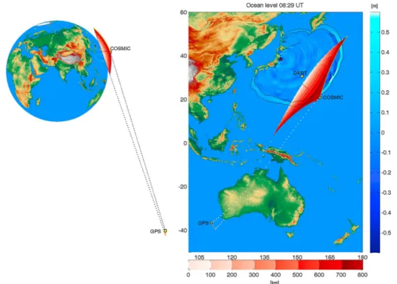
Figure 1. Geometry of the occultation between the satellites GPS 21 and COSMIC 001. (left) Side view of the
occulta-tion region. (right) Map view of the same occultaocculta-tion showing the posiocculta-tion of the tsunami at the time of the occultaocculta-tion. The position of DART #21413 is indicated by a yellow diamond. The trajectories of the satellites are indicated by orange lines starting with an yellow square indicating the position of the satellites at the beginning of the occultation: GPS is Southwest of Australia and COSMIC at the East of Japan. A model of the tsunami wave amplitude in the ocean is represented in blue-cyan color. The part of the ionosphere observed during the occultation is indicated in shades of red that correspond to the altitude above the sea level along the rays between the two satellites. The overlying red line in its center indicates the position of the impact parameter used to define the altitude of each sounding ray.
signal can be modeled with better than 20% accuracy with normal mode summations techniques. This obser-vation might pave the way for space based improvement of the global tsunami warning systems, by enabling space based global observations in the open ocean.
2. Radio Occultation Observation
An ionospheric occultation occurs when a LEO satellite receives a GPS satellite signal, after it has crossed the Earth atmosphere at altitudes lower than the LEO orbit, i.e., through layers of the atmosphere that are below both satellites. Geometrically, this happens when an antenna facing down on the LEO satellite receives the signal from a GPS satellite located on the opposite side of the Earth, as shown in Figure 1. Satellites of the Constellation Observing System for Meteorology Ionosphere and Climate (COSMIC) are on orbits with an inclination of 72◦at 800 km altitude [Anthes et al., 2008]. This altitude is much higher than the peak of the ionosphere electron density, approximately 350 km; therefore, the whole ionosphere is sounded during an occultation event. An occultation event can be setting or rising, if the LEO observes the GPS while it is setting at its horizon or rising above it. Since the LEO period is about 100 min, an occultation lasts about 10 min. The section of the ionosphere sounded at an altitude lower than the LEO becomes larger as the GPS satellites is seen at lower elevation angle. In the equatorial region, two successive occultations between the same satellites occur at about 3000 km of distance, while during the corresponding 100 min time a tsunami propagates only about 1111 km in a 3.5 km depth ocean. This enables even a single LEO satellite to scan efficiently the oceans at a speed twice faster than the tsunami propagation speed.
Occultation rays between the GPS and the LEO are weakly sensitive to the variation of the speed of light inside the ionosphere and can be assumed as straight lines between the two satellites. The nearest point to the Earth center of each ray is defined as its impact parameter [Schreiner et al., 1999]. When the GPS satellite observed from the LEO is at an elevation angle of 0◦the impact parameter coincide with the LEO position,
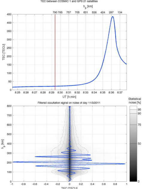
Figure 2. Occultation signal. (top) Time series of TEC between GPS 21 and COSMIC 001, the red line indicates the
beginning of the occultation. The height scale on top indicates the altitude of the impact parameter. (bottom) Gravity wave signal generated by the tsunami. The filtered TEC is represented as function of the altitude of the impact parameter and is compared with the statistical TEC noise of the same day.
and when the elevation angle is negative, the impact parameter is below the LEO altitude. The deeper the impact parameter, the further it is from the LEO satellite. Impact parameters at an altitude of 200 km are 3000 km away from LEO satellites, and the total length of the occultation ray is more than 6000 km in the atmosphere layers below the LEO. In Figure 1 the impact parameters are shown as a red line at the center of the red-shaded area indicating the region of the atmosphere sounded during the occultation. By receiving GPS signals at the two carrier frequencies L1 and L2, it is possible to measure the dispersion of radio signals due to their interaction with the free electrons in the ionosphere. This dispersion is proportional to the total number of free electrons along the signal raypath: the Total Electron Content (TEC) between the GPS and LEO satellites. During a setting occultation, TEC starts at a low value of about 10–20 total electron content unit (TECU, 1 TECU= 1016m−2) that corresponds to the TEC in the upper part of the ionosphere and plasmasphere
at altitude higher than the LEO. It then increases while the impact parameters lowers at altitudes near and below the maximum electron density of the ionosphere, reaching values as high as 100 to 600 TECU. It then decreases to about half of its maximum value before the end of the occultation (Figure 2, top). The reverse is observed during a rising occultation.
Earth and Space Science
10.1002/2014EA000054
From this general characteristics of TEC during occultations it appears clear that the effects of traveling ionospheric disturbances (TID), usually of the order of 0.1 to 1 TECU when observed using ground-based GPS receivers, are extremely small compared to the TEC between two satellites in occultation. Nevertheless, the sensitivity of the GPS phase measurements allows to detect variations with amplitudes of the order of 10−3–10−4 of the diurnal TEC variation [Afraimovich et al., 2001], thus allowing to identify such small
amplitudes. In addition, an occultation event scans the ionosphere through nearly horizontal slices, making it suitable to detect gravity waves that have a large horizontal wavelength. If the link between the LEO and the GPS is nearly parallel to the wave fronts, the amplitude observed through occultation could be large enough to be detected.
Ionospheric occultation data are available at 1 s sampling as level 1.b podTEC files in the University Corporation for Atmospheric Research (UCAR)/COSMIC database. For this study we analyzed only the TEC data recorded when the satellites were in occultation, considering the geographical position and altitude of the impact parameter, in order to select occultations crossing areas near the tsunami. Since the altitude of the impact parameter is the minimum height of each raypath LEO-GPS, it is expected to find a gravity wave signal on data having an impact parameter lower than 300 km, and usually below the maximum value of occultation TEC. To understand whether a TEC signal generated by the tsunami, of a magnitude that is generally lower than 1 TECU, can be recognized in the occultation data, we used separately the data from the 10 to 13 March 2011 to make statistical analyses of the TEC noise during occultation events. First, the TEC values recorded during the occultation were filtered with a band pass filter between 50 mHz and 0.1 Hz, which allows identification of vertical wavelengths between about 5 km and 50 km in the lowermost part of the occultation. At lower frequencies, the filter is affected by the peak or the TEC signal, which corresponds to the crossing of the region of maximum ionization. The temporal filtering was preferred to spatial filtering, as the acquisitions are made with a constant sampling time, that does not correspond to a constant distance in altitude of the impact parameter, which moves faster the more it approaches the Earth’s surface. Filtered TEC usually reveal some oscillations, a signature of plasma fluctuations and irregularities within the occultation area. The envelope of the filtered TEC was used to statistically analyze the TEC noise of 24 h of occultations. At each altitude the TEC amplitudes were used to calculate the percentiles 50, 75, 90, and 95%, represented as background in Figure 2, and provided for each day as supporting information Figures S1 to S4. We observed that during all days more than 50% of occultations have a TEC noise below 0.05 TECU at any altitude, despite of the fact that it was a geomagnetic active period. The highest percentiles show a variation in altitude that recalls the shape of an electron density profile with two maxima: around 100 km and 300 km. A rather pronounced minimum is found around 150 km. But each occultation may individually have different vertical variations, sometimes with maxima for impact parameters above 600 km.
3. Gravity Wave Detected Near the Tsunami
We studied the occultation data of the COSMIC satellites occurring in the vicinity of the tsunami wave front during its propagation through the Pacific Ocean. For 11 March 2011, data are available for three COSMIC satellites for a total of 1072 occultations. Filtered TEC from the occultations that occurred over the Pacific Ocean on 11 March 2011 were analyzed by comparing them with the statistical noise. In the early hours of propagation, the tsunami wave front covered a relatively small area of the ocean and the impact parameters of the few occultations that occurred in this region did do not pass through it. An occultation with a very favorable viewing geometry, parallel to the wave front of the tsunami in the south-north direction, occurred from 08:29 to 08:38 UT between the COSMIC satellite 001 and GPS 21, with the impact parameter being always above the tsunami in the region southeast from Japan (Figure 1). This is a case of occultation where the two satellites are almost orbiting on the same plane: the impact parameter path covers a narrow region in longitude and latitude. We filtered the TEC with a band pass filter between 50 mHz and 0.1 Hz. The maximum amplitude of this signal exceeds 1 TECU when the impact parameter is at 200 km height, an amplitude 2 times larger than the 95% noise level in this frequency band for altitudes between 100 and 300 km (Figure 2). For this occultation, a decrease of amplitude around 150 km is not observed, unlike the majority of the occultations. These characteristics are an indication of a signal of origin outside the ionosphere, consistent with the characteristics of the gravity wave excited by the tsunami.
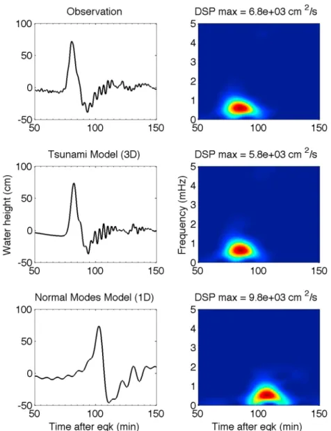
Figure 3. Tsunami data and model comparison. (left column, from top to bottom) Water height measured by DART buoy
#21413 (see location in Figure 1) after the Tohoku-Oki earthquake, modeled using a 3-D model [Bletery et al., 2014] and using a 1-D model (this study). All time series are filtered from 0.2 to 2 mHz. Note the∼ 25min delay between the 1-D model and the DART data, while the 3-D model shows a good agreement. (right column) Corresponding spectrograms.
4. Normal Modes Modeling of the TEC Occultation Signals
Direct modeling allows to understand the coupling mechanism from the ocean to the upper atmosphere. Since the first model that described the propagation of gravity waves in the atmosphere [Pitteway and Hines, 1963], it has been clear that the decrease of the atmosphere density and the consequent increase of wave amplitude, made the upper atmosphere a good medium where to detect the propagation of gravity wave. After the 2004 Sumatra tsunami, models that propagated the ocean surface motion up to the ionosphere allowed to validate ionospheric observation from altimetry satellites [Occhipinti et al., 2006; Mai and Kiang, 2009] and to understand the effect of the geomagnetic field on the coupling strength between the moving neutral atmosphere and the charged particles [Occhipinti et al., 2008]. A spectral full-wave model of the gravity waves excited by a tsunami [Hickey et al., 2009] allowed to predict the airglow signature [Hickey et al., 2010] that was later observed for the first time during this Tohoku event [Makela et al., 2011; Occhipinti et al., 2011]. The modeling of tsunamis through one dimensional (1-D) normal mode summation is a fast and efficient technique [Ward, 1980; Okal, 1982]. As opposed to the above techniques, it requires only the earthquake source model and enables the modeling of the propagation in all parts of the Earth, taking therefore not only
Earth and Space Science
10.1002/2014EA000054
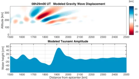
Figure 4. Cross section of the modeled tsunami-induced gravity wave. (top) Total displacement of the air parcels.
(bottom) Modeled tsunami water displacement. This section is oriented along a radial direction from the earthquake epicenter at135◦azimuth, between (28.76◦N,153.84◦E) and (22.40◦N,160.09◦E). The tsunami propagation is from left to right. The maximum displacement of 25 km is compatible with the amplitude of TID measured from ground-based GPS stations during the 26 December 2004 Sumatra tsunami that were of the order of 17.2 km [Liu et al., 2006].
the influence of the solid Earth on the tsunami propagation [Watada et al., 2014] but also its interaction and further propagation in the atmosphere. It is, however, unable to model the effects of bathymetry changes and therefore the precise arrival time of the tsunami at any location. Point source dislocation models strongly overestimate the amplitude of the tsunami, as they do not model the interferences of the tsunami at the source. A better model of the source is therefore necessary. Here we used the updated United States Geological Survey (USGS) finite fault model [Hayes, 2011]. It provided a good estimation of the tsunami amplitude and wave form, as shown by Figure 3.
We modeled the tsunami ionospheric signal by computing the tsunami-coupled gravity normal modes of the Earth/Ocean/atmosphere system, following the theory developed by Lognonné et al. [1998]. This modeling approach, including the coupling with the ionosphere, is described in detail by Rolland et al. [2011b] for Rayleigh waves and it is used here for the first time for tsunami-induced gravity waves of the Earth-Ocean-Atmosphere system.
We started from the Preliminary Reference Earth Model (PREM) [Dziewonski and Anderson, 1981] overlaid by the ocean. An ocean depth of 3.5 km was used to represent the average depth in the region below the occul-tation impact parameter. On top of the ocean, the atmosphere physical parameters were modeled using the Naval Research Laboratory Mass Spectrometer and Incoherent Scatter Radar (NRLMSISE-00) [Picone et al., 2002] atmosphere model. The effects of atmospheric viscosity were included following Artru et al. [2001]. The vertical profiles of atmospheric parameters (density, temperature, sound speed, and viscosity) were computed at the time and location of the Tohoku event.
To assess the overall model, we compared in Figure 3 the tsunami amplitude derived from the 1-D tsunami-coupled normal modes summation at that position with the sea level anomaly measured by the pressure sensor connected to the Deep-ocean Assessment and Reporting of Tsunamis (DART) buoy #21413. As for the oceanic tsunami, the 1-D approach, based on a spherically symmetric structure, does not take into account the large variation in bathymetry which leads to large variations of the tsunami arrival time and local amplitude. We obtained a difference of about 25 min in arrival time but an amplitude and waveform very similar to the one observed at the DART buoy #21413, that was located in the direction of the main direc-tional lobe of the tsunami. The time discrepancy has been corrected for the ionospheric modeling by shifting the synthetics to maximize their cross correlation with experimental occultation data. This approach enables, however, a very accurate modeling of the coupling effects between the ocean and the atmosphere, and of the neutral velocity 3-D vector of the tsunami-coupled gravity wave at ionospheric height. A cross section of the total displacement of the air parcels at ionospheric height along with the ocean wave is shown in Figure 4 and an animation is provided in the supporting information (Movie S1). The velocity of the neutral
Figure 5. Comparison of the occultation data with synthetics. (top) Band pass filtered, between 0.05 Hz and 1 Hz.
(bottom) Band pass filtered between 0.05 Hz and 0.07 Hz.
atmosphere is then converted in electron (or ion) velocity, using Hooke [1970] approximation, which finally provide a plasma wind parallel to the magnetic field and equal to the projection of the neutral wind on the magnetic field direction, vi= (u.1b)1b, where u and 1bare the neutral velocity vector and the magnetic field
unit vector respectively. The 3-D time varying electron density field is then computed from the conservation of electrons equation, assuming therefore marginal ionization or recombination processes associated with the tsunami perturbation. The electron density perturbation was computed on a grid covering from 22◦to 30◦in latitude, 149◦to 157◦in longitude, and 100 km to 400 km in altitude. This enables the last modeling step, in which the TEC is computed by integrating the electron density perturbation between the locations of the GPS and COSMIC satellites, for all recorded times.
A filtering of the raw TEC data is required in order to isolate the tsunami signal. Filtering the TEC data in the time domain at a given frequency f can be considered as roughly equivalent to an horizontal filtering with wavelength𝜆H = VC∕f and a vertical filtering with wavelength𝜆r = VC(rC− rs)∕(frs), where VCis the
orbital velocity of the COSMIC satellite (7.45 km/s), rCis the radius of the COSMIC orbit, and rsthe radius of
the sounded tsunami-driven ionospheric perturbation. Most of the filtering leads therefore into horizontal filtering, as (rC− rs)∕rs = 0.083 for a sounding altitude of 250 km and an orbit height of 800 km. The
veloc-ity of the satellite and the tsunami are, respectively,√g(rC)rCand√g(a)H, where g(r) is the Earth gravity
at radius r, H the ocean depth, and a the mean radius of the Earth. The TEC signal frequency f is therefore equivalent to tsunami frequency ftsu= f
√
HrC
a2 ∼ 0.025f. Figure 5 shows the comparison between observed
and modeled TEC for two different bandwidths: the first is for bandwidth 0.05 Hz–1 Hz, while the second is for 0.05 Hz–0.07 Hz, which correspond therefore to tsunami frequency bandwidth of 1.25 mHz–25 mHz and 1.25 mHz–1.75 mHz. The second is in the typical bandwidth in which ground-based GPS observations have been already reported (e.g., Rolland et al. [2011b] used a bandwidth of 1–2 mHz and obtained a signature peaking at ∼ 1.5 mHz for three events of different sizes). In this second bandwidth, we note a good agreement in waveform and amplitude. The highest correlation of 0.8 is obtained for a 17.12 s time delay, meaning that the radio occultation data are slightly ahead from the synthetics. We attribute this excellent overall agreement to the large extent of the sounded gravity wave. This acts averaging the tsunami response, well reproduced by a 1-D Earth/Ocean/Atmosphere model with 3.5 km water depth and the extended USGS finite-fault model as excitation source. We expect that taking into account the lateral variations of the bathymetry will allow extending this agreement over a larger bandwidth.
The occultation is simulated from bottom to top, and we note some amplitude discrepancies at the beginning of the occultation, which can be explained by an overestimation of the attenuation (or underestimation of
Earth and Space Science
10.1002/2014EA000054
the TEC) at altitude much higher than the altitude of the maximum of the tsunami-induced atmospheric perturbation, which is about 250 km.
5. Conclusions
The first experimental radio occultation observation of a gravity wave excited by a tsunami has been possible during the 11 March 2011 Tohoku event. Due to the small amplitude of the gravity wave signal compared to the TEC between the two occulting satellites, we used a tsunami-coupled normal modes model applied to the Earth with ocean and a realistic atmosphere, including the effects of viscosity in the upper atmosphere. Model results show a good agreement both in period and amplitude with the experimental observations, and amplitudes about 10 times larger than those of the median (i.e., 50%) traveling ionospheric disturbances. This result demonstrates that it is possible to use satellite radio occultation measurements to detect tsunami-induced perturbations of the ionosphere.
Additional observations are still needed to confirm that even in the case of smaller events the ionospheric signature of the induced gravity wave can be discriminate from the ambient noise. The number of satellites in orbit allowing continuous radio occultation observation is still very limited and does not allow a continuous global coverage. Nevertheless, it can be foreseen that future constellations of radio occultation satellites, taking advantage of the multiple GNSS constellations, or cheaper constellations of dedicated nanosatellites could be able to detect the ionospheric signature of moderate to large tsunamis and therefore be a valuable support for tsunami monitoring and warning systems.
References
Afraimovich, E., A. Altynsev, V. Grechnev, and L. Leonovich (2001), Ionospheric effects of the solar flares as deduced from global GPS network data, Adv. Space Res., 27(6–7), 1333–1338, doi:10.1016/S0273-1177(01)00172-7.
Anthes, R. A., et al. (2008),The COSMIC/FORMOSAT-3 mission: Early results, Bull. Am. Meteorol. Soc., 89(3), 313–333, doi:10.1175/BAMS-89-3-313. Artru, J., P. Lognonné, and E. Blanc (2001), Normal modes modelling of post-seismic ionospheric oscillations, Geophys. Res. Lett., 28(4), 697–700,
doi:10.1029/2000GL000085.
Artru, J., V. Ducic, H. Kanamori, P. Lognonné, and M. Murakami (2005), Ionospheric detection of gravity waves induced by tsunamis, Geophys. J. Int., 160 (3), 840–848, doi:10.1111/j.1365-246X.2005.02552.x.
Astafyeva, E., K. Heki, V. Kiryushkin, E. Afraimovich, and S. Shalimov (2009), Two-mode long-distance propagation of coseismic ionosphere disturbances, J. Geophys. Res., 114, A10307, doi:10.1029/2008JA013853.
Astafyeva, E., P. Lognonné, and L. Rolland (2011), First ionospheric images of the seismic fault slip on the example of the Tohoku-oki earthquake, Geophys. Res. Lett., 38, L22104, doi:10.1029/2011GL049623.
Astafyeva, E., L. Rolland, P. Lognonné, K. Khelfi, and T. Yahagi (2013), Parameters of seismic source as deduced from 1 Hz ionospheric GPS data: Case study of the 2011 Tohoku-oki event, J. Geophys. Res. Space Physics, 118, 5942–5950, doi:10.1002/jgra.50556.
Bletery, Q., A. Sladen, B. Delouis, M. Vallée, J.-M. Nocquet, L. Rolland, and J. Jiang (2014), A detailed source model for theMw9.0 Tohoku-Oki earthquake reconciling Geodesy, seismology and tsunami records, J. Geophys. Res. Solid Earth, 119, 7636–7653, doi:10.1002/2014JB011261. Ducic, V., J. Artru, and P. Lognonné (2003), Ionospheric remote sensing of the Denali earthquake Rayleigh surface waves, Geophys. Res. Lett.,
30 (18), 1951, doi:10.1029/2003GL017812.
Dziewonski, A. M., and D. L. Anderson (1981), Preliminary reference Earth model, Phys. Earth. Planet. Inter., 25(4), 297–356, doi:10.1016/0031-9201(81)90046-7.
Galvan, D. A., A. Komjathy, M. P. Hickey, P. Stephens, J. Snively, Y. Tony Song, M. D. Butala, and A. J. Mannucci (2012), Ionospheric signatures of Tohoku-Oki tsunami of March 11, 2011: Model comparisons near the epicenter, Radio Sci., 47, RS4003, doi:10.1029/2012RS005023. Garcia, R. F., E. Doornbos, S. Bruinsma, and H. Hebert (2014), Atmospheric gravity waves due to the Tohoku-Oki tsunami observed in the
thermosphere by GOCE, J. Geophys. Res. Atmos., 119, 4498–4506, doi:10.1002/2013JD021120.
Hayes, G. P. (2011), Rapid source characterization of the 2011Mw9.0 off the Pacific coast of Tohoku earthquake, Earth Planets Space, 63(7), 529–534, doi:10.5047/eps.2011.05.012.
Hickey, M. P., G. Schubert, and R. L. Walterscheid (2009), Propagation of tsunami-driven gravity waves into the thermosphere and ionosphere, J. Geophys. Res., 114, A0834, doi:10.1029/2009JA014105.
Hickey, M. P., G. Schubert, and R. L. Walterscheid (2010), Atmospheric airglow fluctuations due to a tsunami-driven gravity wave disturbance, J. Geophys. Res., 115, A06308, doi:10.1029/2009JA014977.
Hooke, W. H. (1970), The ionospheric response to internal gravity waves: 1. TheF2region response, J. Geophys. Res., 75(28), 5535–5544, doi:10.1029/JA075i028p05535.
Kakinami, Y., M. Kamogawa, S. Watanabe, M. Odaka, T. Mogi, J.-Y. Liu, Y.-Y. Sun, and T. Yamada (2013), Ionospheric ripples excited by superimposed wave fronts associated with Rayleigh waves in the thermosphere, J. Geophys. Res. Space Physics, 118, 905–911, doi:10.1002/jgra.50099.
Kherani, E. A., P. Lognonné, H. Hébert, L. Rolland, E. Astafyeva, G. Occhipinti, P. Co¨ısson, D. Walwer, and E. R. de Paula (2012), Modelling of the total electronic content and magnetic field anomalies generated by the 2011 Tohoku-Oki tsunami and associated acoustic-gravity waves, Geophys. J. Int., 191(3), 1049–1066, doi:10.1111/j.1365-246X.2012.05617.x.
Komjathy, A., D. A. Galvan, P. Stephens, M. D. Butala, V. Akopian, B. Wilson, O. Verkhoglyadova, A. J. Mannucci, and M. Hickey (2012), Detecting ionospheric TEC perturbations caused by natural hazards using a global network of GPS receivers: The Tohoku case study, Earth Planets Space, 64 (12), 1287–1294, doi:10.5047/eps.2012.08.003.
Liu, J.-Y., Y.-B. Tsai, K.-F. Ma, Y.-I. Chen, H.-F. Tsai, C.-H. Lin, M. Kamogawa, and C.-P. Lee (2006), Ionospheric GPS total electron content (TEC) disturbances triggered by the 26 December 2004 Indian Ocean tsunami, J. Geophys. Res., 111, A085303, doi:10.1029/2005JA011200. Acknowledgments
This work has been supported by the French Space Agency CNES (R&D Sondage ionosphérique par radio occultation et réflectométrie, R-S10/OT-0002-058), by the French National Research Agency (ANR) TO-EOS project ANR-11-JAPN-008 and by the United States Office of Naval Research (ONR) Global under contract TWIST (N000141310035). We thank the UCAR/COSMIC program for the COSMIC data available in the COSMIC Data Analysis and Archival Center (CDAAC): http://cosmic-io.cosmic.ucar. edu/cdaac/. We thank NOAA National Geophysical Data Center for the DART buoys data available at http://www. ndbc.noaa.gov/dart.shtml. We thank Quentin Bletery and Anthony Sladen for providing us with the tsunami model data shown in Figures 1 and 3. This is IPGP contribution 3613.
Liu, J.-Y., C.-H. Chen, C.-H. Lin, H.-F. Tsai, C.-H. Chen, and M. Kamogawa (2011), Ionospheric disturbances triggered by the 11 March 2011 M9.0 Tohoku earthquake, J. Geophys. Res., 116, A06319, doi:10.1029/2011JA016761.
Lognonné, P., E. Clévédé, and H. Kanamori (1998), Computation of seismograms and atmospheric oscillations by normal-mode summation for a spherical earth model with realistic atmosphere, Geophys. J. Int., 135(2), 388–406, doi:10.1046/j.1365-246X.1998.00665.x.
Lognonné, P., J. Artru, R. Garcia, F. Crespon, V. Ducic, E. Jeansou, G. Occhipinti, J. Helbert, G. Moreaux, and P.-E. Godet (2006), Ground-based GPS imaging of ionospheric post-seismic signal, Planet. Space Sci., 54 (5), 528–540, doi:10.1016/j.pss.2005.10.021.
Mai, C.-L., and J.-F. Kiang (2009), Modeling of ionospheric perturbation by 2004 Sumatra tsunami, Radio Sci., 44, RS3011, doi:10.1029/2008RS004060.
Makela, J. J., et al. (2011), Imaging and modeling the ionospheric airglow response over Hawaii to the tsunami generated by the Tohoku earthquake of 11 March 2011, Geophys. Res. Lett., 38, L00G02, doi:10.1029/2011GL047860.
Maruyama, T., T. Tsugawa, H. Kato, A. Saito, Y. Otsuka, and M. Nishioka (2011), Ionospheric multiple stratifications and irregularities induced by the 2011 Tohoku earthquake, Earth Planets Space, 63(7), 863–873, doi:10.5047/eps.2011.06.008.
Nishitani, N., T. Ogawa, Y. Otsuka, K. Hosokawa, and T. Hori (2011), Propagation of large amplitude ionospheric disturbances with velocity dispersion observed by the SuperDARN Hokkaido radar after the 2011 off the Pacific coast of Tohoku earthquake, Earth Planets Space, 63(7), 891–896, doi:10.5047/eps.2011.07.003.
Occhipinti, G., P. Lognonné, E. A. Kherani, and H. Hébert (2006), Three-dimensional waveform modeling of ionospheric signature induced by the 2004 Sumatra tsunami, Geophys. Res. Lett., 33, L20104, doi:10.1029/2006GL026865.
Occhipinti, G., E. A. Kherani, and P. Lognonné (2008), Geomagnetic dependence of ionospheric disturbances induced by tsunamigenic internal gravity waves, Geophys. J. Int., 173(3), 753–756, doi:10.1111/j.1365-246X.2008.03760.x.
Occhipinti, G., P. Co¨ısson, J. J. Makela, S. Allgeyer, A. Kherani, H. Hébert, and P. Lognonné (2011), Three-dimensional numerical modeling of tsunami-related internal gravity waves in the Hawaiian atmosphere, Earth Planets Space, 63(7), 847–851, doi:10.5047/eps.2011.06.051. Occhipinti, G., L. Rolland, P. Lognonné, and S. Watada (2013), From Sumatra 2004 to Tohoku-Oki 2011: The systematic GPS detection of the
ionospheric signature induced by tsunamigenic earthquakes, J. Geophys. Res. Space Physics, 118, 3626–3636, doi:10.1002/jgra.50322. Ogawa, T., N. Nishitani, T. Tsugawa, and K. Shiokawa (2012), Giant ionospheric disturbances observed with the SuperDARN Hokkaido HF radar
and GPS network after the 2011 Tohoku earthquake, Earth Planets Space, 64 (12), 1295–1307, doi:10.5047/eps.2012.08.001.
Okal, E. A. (1982), Mode-wave equivalence and other asymptotic problems in tsunami theory, Phys. Earth. Planet. Inter., 30(1), 1–11, doi:10.1016/0031-9201(82)90123-6.
Picone, J. M., A. E. Hedin, D. P. Drob, and A. C. Aikin (2002), NRLMSISE-00 empirical model of the atmosphere: Statistical comparisons and scientific issues, J. Geophys. Res., 107(A12), 1468, doi:10.1029/2002JA009430.
Pitteway, M. L. V., and C. O. Hines (1963), The viscous damping of atmospheric gravity waves, Can. J. Phys., 41(12), 1935–1948.
Rolland, L. M., G. Occhipinti, P. Lognonné, and A. Loevenbruck (2010), Ionospheric gravity waves detected offshore Hawaii after tsunamis, Geophys. Res. Lett., 37, L17101, doi:10.1029/2010GL044479.
Rolland, L. M., P. Lognonné, E. Astafyeva, E. A. Kherani, N. Kobayashi, M. Mann, and H. Munekane (2011a), The resonant response of the iono-sphere imaged after the 2011 off the Pacific coast of Tohoku Earthquake, Earth Planets Space, 63(7), 853–857, doi:10.5047/eps.2011.06.020. Rolland, L. M., P. Lognonné, and H. Munekane (2011b), Detection and modeling of Rayleigh wave induced patterns in the ionosphere,
J. Geophys. Res., 116, A05320, doi:10.1029/2010JA016060.
Schreiner, W. S., S. V. Sokolovskiy, C. Rocken, and D. C. Hunt (1999), Analysis and validation of GPS/MET radio occultation data in the ionosphere, Radio Sci., 34(4), 949–966, doi:10.1029/1999RS900034.
Ward, S. N. (1980), Relationships of tsunami generation and an earthquake source, J. Phys. Earth, 28(5), 441–474, doi:10.4294/jpe1952.28.441. Watada, S., S. Kusumoto, and K. Satake (2014), Traveltime delay and initial phase reversal of distant tsunamis coupled with the self-gravitating
elastic Earth, J. Geophys. Res. Solid Earth, 119 (5), 4287–4310, doi:10.1002/2013JB010841.
Erratum
In the originally published version of this article, the supporting figure files were in an incorrect format. The files have since been corrected, and this version may be considered the authoritative version of record.