Série Scientifique
Scientific Series
Nº 95s-26
INDUSTRY-SPECIFIC CAPITAL AND THE WAGE PROFILE: EVIDENCE
FROM THE NLSY AND THE PSID
Daniel Parent
Montréal Avril 1995
Ce document est publié dans lintention de rendre accessible les résultats préliminaires de la recherche effectuée au CIRANO, afin de susciter des échanges et des suggestions. Les idées et les opinions émises sont sous lunique responsabilité des auteurs, et ne représentent pas nécessairement les positions du CIRANO ou de ses partenaires.
This paper presents preliminary research carried out at CIRANO and aims to encourage discussion and comment. The observations and viewpoints expressed are the sole responsibility of the authors. They do not necessarily represent positions of CIRANO or its partners.
CIRANO
Le CIRANO est une corporation privée à but non lucratif constituée en vertu de la Loi des compagnies du Québec. Le financement de son infrastructure et de ses activités de recherche provient des cotisations de ses organisations-membres, dune subvention dinfrastructure du ministère de lIndustrie, du Commerce, de la Science et de la Technologie, de même que des subventions et mandats obtenus par ses équipes de recherche. La Série Scientifique est la réalisation dune des missions que sest données le CIRANO, soit de développer lanalyse scientifique des organisations et des comportements stratégiques.
CIRANO is a private non-profit organization incorporated under the Québec Companies Act. Its infrastructure and research activities are funded through fees paid by member organizations, an infrastructure grant from the Ministère de lIndustrie, du Commerce, de la Science et de la Technologie, and grants and research mandates obtained by its research teams. The Scientific Series fulfils one of the missions of CIRANO: to develop the scientific analysis of organizations and strategic behaviour.
Les organisations-partenaires / The Partner Organizations
Ministère de lIndustrie, du Commerce, de la Science et de la Technologie. École des Hautes Études Commerciales.
École Polytechnique. Université de Montréal. Université Laval. McGill University.
Université du Québec à Montréal. Bell Québec.
La Caisse de dépôt et de placement du Québec. Hydro-Québec.
Banque Laurentienne du Canada.
Fédération des caisses populaires de Montréal et de lOuest-du-Québec. Téléglobe Canada.
Société délectrolyse et de chimie Alcan Ltée. Avenor.
CIDEM.
This paper is a revised version of chapter 3 of my Ph. D. dissertation submitted to the Université de %
Montréal in December 1994. Special thanks to my supervisors, Thomas Lemieux and Bentley MacLeod, for their comments, suggestions and general guidance. Hank Farber also contributed with useful suggestions. Financial support from the SHRCC is also gratefully acknowledged.
Industry-Specific Capital and the
Wage Profile: Evidence from the
NLSY and the PSID
%
Daniel Parent
Abstract / Résumé
Using data from the NLSY (1979-1991) and from the Panel Study of Income Dynamics (PSID, 1981-1987), we seek to determine whether there is any net positive return to tenure with the current employer once we control for industry-specific capital. Using data from the PSID, Topel (JPE 1991) concluded that 10 years of seniority with an employer translated into a net return of about 25%. However, once we include total experience in the industry as an additional explanatory variable, the return to seniority vanishes almost completely when we use either OLS, GLS or IV-GLS estimation methods, although this conclusion varies somewhat according to the occupation, some occupation classes showing a negative net return to tenure and others showing a positive net return. Note also that this result holds whether the analysis is carried out at the 1-digit, 2-digit or 3-2-digit level. Therefore, it seems that what matters most for the wage profile in terms of human capital is not so much firm-specificity but industry-specificity.
Avec les données du NLSY ainsi que celles du Panel Study of Income Dynamics (PSID), on cherche à déterminer sil y a un rendement positif net lié à lancienneté dans la firme. Topel (JPE 1991) a montré avec un échantillon du PSID lexistence dun rendement substantiel (25 % en 10 ans). Toutefois, du moment que lon inclut lexpérience dans lindustrie courante dans léquation de salaire (en plus de lancienneté dans la firme ainsi que lexpérience totale de travail), leffet dancienneté disparaît presque complètement, que lon estime par simples moindres carrés généralisés ou par la méthode des variables instrumentales (IV-GLS), et ce, avec les deux échantillons différents. À noter également que ce résultat est robuste au degré dagrégation des classes dindustries.
See also Neal (1993) for a different approach to assessing the degree of industry-specificity.
1
For a theoretical model that describes the wage (price) formation process in the presence of renegotiation
2
and relation-specific investments, see MacLeod and Malcomson (1993a,b). Under certain conditions and when proper allowance is made for the possibility of contract renegotiation, they show that employers need not offer their workers above market-clearing wages.
The response rate was at 71% in 1991.
3
I. Introduction
The extent to which wages rise with years of seniority with the same employer has been the subject of some controversy over the last few years (e.g Topel (1991); Altonji and Shakotko (1987); Abraham and Farber (1987), Abowd, Kramarz and Margolis (1994)). Much of the debate surrounding this issue has focused on the appropriate econometric methods to be used to handle the issue of the endogeneity of the tenure variable. However, virtually no attention has been paid to the question of whether it is appropriate to decompose a workers total labor market experience into only two components, tenure with the current employer and total prior experience (or total experience including tenure if one wants to obtain the latters net effect). With data from the National Longitudinal Survey of Youth (NLSY) and from the Panel Study of Income Dynamics (PSID), it is shown that simply by adding total experience in the current industry as an additional explanatory variable, the net tenure effect vanishes almost completely. This suggests that past studies (most notably Topel (1991)) have overlooked an important factor in analyzing the effect of tenure on wages. It is worth noting that this result holds when the analysis is carried out either at the one-digit, two-digit, or three-digit level. Therefore, it seems that what matters most for the wage profile in terms of human capital is not so much firm-specificity but industry-specificity.1
These results lead to the following basic conclusion: for these two samples of workers, the wage formation process seems to be very competitive with no solid evidence of rent sharing over the return on firm-specific capital. Or, put in the language of bargaining theory, there is little evidence that the workers represented in these two samples are paid much in excess of their outside option.2
II. The Data
The National Longitudinal Survey of Youth data set surveyed 12,686 young males and females who were between the age of 14 and 21 in 1979 . It contains3 detailed employment histories of the respondents thereby permitting the construction
The choice of six years as a cutoff point is arbitrary, and hence debatable. The idea is to exclude those that
4
make quasi-permanent transitions and who might be considering returning to school a few years down the road. It seems reasonable to assume that few people would enter the labor market while planning to leave it in six years or more to go back to school. The same could not be said if we were considering a one to three year (say) horizon. In any event, the results were left unchanged if all school returners were excluded.
This PSID extract was kindly supplied by Robert Valetta who used it in his paper with David Brownstone
5
(Brownstone and Valetta (1993)) on the modeling of measurement error bias in wage equations.
(1) of relatively error-free variables for tenure as well as for the total experience accumulated since the beginning of ones full time transition to the labor market. At the time this project was started, data were available from 1979 to 1991.
The people who were considered as having entered the labor market on a full-time basis were (i) those whose primary activity was either working full-time, on a temporary lay-off or looking actively for a job, (ii) those who did not return to school on a full-time basis within six years and (iii) those who had worked at least half the4 year since the last interview and who were working at least 20 hours per week. Individuals excluded from the sample are those younger than 18, those that had been in the military at any time, the self-employed, the ones whose jobs were part of a government program and the ones working without pay, those who were in the farming business and also all public sector employees. We are then left with 29,020 observations. Some summary statistics of the sample are provided in table 1.
Turning now to the Panel Study of Income Dynamics (PSID), the sample consists of heads of households aged 18 to 64 with positive earnings for the period spanning the years 1981-1987. The question of whether people have entered the labor5 market on a full-time basis is obviously less of a concern for this sample of older workers. Summary statistics are provided in table 2.
III. Results
III.1 Basic Model.
(2) where w represents the real hourly wage of person i in job j in industry k at time t,ijkt T is tenure, Exp is total labor market experience and Expind is total experience in the current industry. Specifically, the variable experience in the industry gives the consecutive number of years one has been in the same industry excluding tenure with the current employer. For example, if a worker leaves her first employer to take another job in the same industry, she adds experience in that industry, whereas if she takes another job in a different industry, her seniority in the industry is accordingly reset to zero. An implicit assumption is that the worker stays in the same industry throughout her employment relationship with a particular employer (the data show that this is not always the case: there are workers who change industry while not changing employers). Still, despite its shortcomings, this variable should give a fairly good idea of the industry effects embedded in the tenure variable. All other covariates, including squared terms for tenure, total experience and industry experience, are ignored for ease of presentation. As in previous studies, unobserved heterogeneity can be decomposed into an individual effect ( " ) and a job-match effect ( 2 ). The person-i ij specific effect can be seen as representing unmeasured aspects of each individuals earning ability while the job-match component represents the unknown (to the econometrician) quality of the employment relationship stemming from search activity, for example. Both of these effects are assumed to be time-invariant. Another unobserved heterogeneity component, ( , which serves the same purpose as the job-ik match component, is added to represent the unobserved quality of the match between the individual and the industry in which he works.
As emphasized in the literature, the problem in estimating equation (1) with ordinary least-squares is that the unobserved components are likely to be correlated with tenure, total labor market experience and also, in our case, total experience in the industry. Those with high "s may have enjoyed careers that were interrupted less frequently by unemployment spells, while better matches (high 2s and high (s) are likely to be formed if you have more experience due to human capital and search effects. Also, tenure and total experience in the current industry are likely to be correlated with their corresponding match quality components. Dropping for the moment the assumption of time-invariant job-match and industry-match components, lets suppose that we can write them as
For simplicity, I also assume that total experience in the industry is not correlated with the job-match
6
component while tenure is not correlated with the unobserved quality of the match in the industry. One could argue that more experience in the industry may help you find a better job-match because of superior information in comparison to a worker who has never worked in the industry.
See also Finnie (1993) for an extension of the method of Altonji and Shakotko to the experience variable.
7
(3) where T and 0 are assumed to be orthogonal to the regressors. The discussionijt ikt 6 above suggests that R and n are positive. In the context of maximizing behavior on2 2 the part of a worker who faces a wage distribution, Topel(1991) argues that R is1 negative once we control for experience, assuming there is a tenure effect. If there is no tenure effect, then R equals zero. Presumably, the same sort of considerations1 apply to n . That is, provided that we control for total labor market experience, the3 quality of the match in the industry should be negatively correlated with the number of years one has been in the same industry. Substituting equation (2) into equation (1) we get
We see from equation (3) that although we are interested in the $s, using ordinary
least-squares will produce estimates of composite effects and the regressors would still be correlated with ". To provide some correction for these problems, I use the instrumental variable (IV) methodology proposed by Altonji and Shakotko (1987) .7 Tenure is instrumented with its deviations from job-match means whereas experience is instrumented with its deviations from individual means. In the same spirit, total experience in the industry is instrumented with its deviations from industry-match means. The instruments for tenure and experience in the industry are, by construction, uncorrelated with their respective match quality components, while the instrument for experience is, also by construction, uncorrelated with the individual component. First differences (as in Topel (91)) were not used to obtain a consistent estimate of the sum of the tenure and experience coefficients, because this would enhance any measurement errors present in the data as compared with using deviations from means. This is further justified by Topels observation that much of the discrepancy between his results and those of Altonji and Shakotko stemmed from measurement errors pertaining to the tenure variable.
Finally, since the same individuals are followed over time, residuals will be serially correlated due to the presence of a fixed individual effect. To provide
All results are obtained using the weighted samples.
8
correction for this problem, all regressions are done using generalized least-squares under the assumption that the error term contains an individual-specific component. III.2 Earnings Equation Estimates.
I now turn to the question of disentangling industry effects from purely firm-specific effects. Note that the analysis is carried out at the 1-digit, 2 digit, and 3-digit8 levels. If the tenure effect is entirely firm-specific, then it should not matter whether you change industry or not: the tenure coefficient should not budge at all. On the other hand, if a portion of the tenure effect reflects the specificity of the human capital acquired on the current job relative to the industry in which the firm operates, then adding such a control should decrease the coefficient on tenure. Using the NLSY data, the results shown in tables 3 and 4 seem to validate the latter explanation: in the GLS specification of the 1-digit case (column (4) in table 3), over 50% of the effect of tenure is accounted for by industry effects. The tenure effect further decreases in the 2-digit case and disappears completely in the 3-digit case (columns (3) and (2), respectively). Once the instrumental variable specification is adopted (see table 4), there is no evidence of a substantial and statistically significant positive tenure effect, even at the 1-digit level. The entire effect is picked up by the variable representing experience in the industry. Note that total experience is only slightly affected by the inclusion of the new variable.
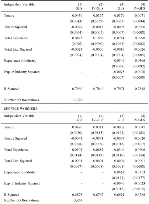
Table 5 provides a breakdown by occupational category. It could be that for managers or professionals, firm-specific investments are more important and that firms would prefer to pay these highly skilled individuals above their outside option rather than to face the prospect of losing them, especially if these workers are in short supply. The results indicate that there is a return to tenure for the category consisting of professionals, technical workers, managers and administrators. In the GLS specification, even after adding experience in the industry, the tenure effect is substantial and significant. In fact, in the IV-GLS specification, the effect is larger after adding the control for industry effects. For the next three categories of workers, the results are similar to those obtained for the total sample: the industry effect is large and significant while the firm effect is not. Again, it is interesting to note that total experience is not markedly affected by the added variable. Total experience and experience in the industry really do seem to provide complementary explanatory power to the wage formation process.
If we admit that investment in firm-specific skills is complementary to the quality of the match, then it
9
follows that older workers who have had more time to sample the job offer distribution would be better candidates for such investments. On the question of complementarity between match quality and firm-specific capital, see Jovanovic (1979).
III.3 Comparison with Data from the PSID
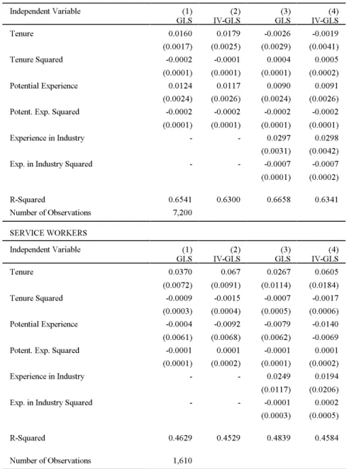
Given that the NLSY is composed of young persons making their transition to the labor market (the oldest individuals in 1991 were 33 years old), it could very well be that the results above are peculiar to that data set. To be more precise, assuming that skills which are truly firm-specific are associated more with older workers than their younger counterparts, then the results above may not hold with a sample of workers who have more mature careers. Therefore, to check whether9 results are robust across data sets, we have estimated the same type of equation with data from the Panel Study of Income Dynamics (PSID). The sample consists of heads of households aged 18 to 64 with positive earnings for the years spanning the period 1981 to 1987. Results are shown in tables 6 and 7. As shown in table 6, the impact of including the additional explanatory variable is qualitatively the same as in the case of the NLSY. With GLS and IV-GLS, adding the control for industry-specific capital has the effect of reducing the tenure coefficient to close to zero. Results by occupational categories are shown in table 8. Contrary to the results obtained with the NLSY, there is no evidence of a return to tenure for professionnals, managers and administrators. For clerical and unskilled workers, there is even evidence of a negative net return to firm seniority. However, for service workers, the estimated return to tenure is sizeable and significant, which is not the case for the NLSY sample. Interestingly, a common denominator of the results with the PSID is that the total experience coefficients are much smaller in comparison with those estimated with the NLSY. Thus, it appears that as workers careers evolve, the skills they acquire are more narrowly defined. Of course, as workers gain experience in the labor market, the search process leads them to more satisfactory matches. Presumably then, the opportunities for investment in more specific skills are enhanced in these better jobs.
IV. Conclusion
With data from the NLSY, it has been shown that by controlling for workers who change industry when they change jobs, the tenure effect is reduced by over 50% at the 1-digit level if generalized least-squares are used, while it disappears completely at the 3-digit level, whether it be with GLS or with the instrumental variable methodology borrowed from Altonji and Shakotko (1987). These results generally
See Hause (1980) for a study linking the covariance of earnings to the theory of human capital.
10
hold when I subdivide the sample by occupational categories, although there is some evidence of a tenure effect for professionals, technical workers and managers. Also, by using data from the PSID, I have shown that these results are robust across data sets and are not peculiar to the young NLSY workers making their full-time transition to the labor market. The basic conclusion to be drawn from these results is that the wage formation process seems to be very competitive for most of the workers in these two data sets.
Having established that the average tenure slope is close to zero, an interesting avenue for future research would be determine whether there is substantial variance in the slopes. Results by occupational categories suggest that there is some variability in the estimated tenure slopes. However, all research up to now has used the assumption of fixed parameters. A more refined analysis would call upon the use of a random coefficient model to study the covariance structure of a log-earnings equation with proper allowance made for the randomness in the tenure and experience profiles. Then we could determine with more confidence whether there is evidence10 of workers receiving wages above their outside option.
References
Abowd, J., F. Kramarz, D. Margolis, High-Wage Workers and High-Wage Firms, INSEE Working Paper, September 1994.
Abraham, K. & H. Farber, Job Duration, Seniority, and Earnings, American Economic Review 77 (June 1987): 278-97.
Altonji, J., & R. Shakotko, Do Wages Rise with Seniority?, Review of Economic Studies 54 (July 1987): 437-59.
Brownstone, D., R. Valetta, Modeling Measurement Error Bias in Cross-Section and Longitudinal Wage Equations, University of California (Irvine) Working Paper, 1993.
Finnie, R, Tenure, Experience, and Mens and Womens Wages: Panel Estimates from the National Longitudinal Survey of Youth, Groupe de Recherche en Politique Economique, cahier de recherche 9305, Université Laval, 1993. Hause, J. C. The Fine Structure of Earnings and the On-the-Job Training
Hypothesis, Econometrica 52: 1013-1030.
Jovanovic, B. Firm-specific Capital and Turnover, Journal of Political Economy 87 (December 1979): 1246-1260.
MacLeod, W. Bentley & J. M. Malcomson, Specific Investment and Wage Profiles in labour Markets, European Economic Review 37, 1993a: 343-354. MacLeod, W. Bentley & J. M. Malcomson, Investment, Holdup, and the Form of
Market Contracts, American Economic Review 83(4), 1993b: 811-837. Neal, D., Industry-Specific Human Capital: Evidence from Displaced Workers,
University of Chicago Working Paper, 1993.
Topel, R. Specific Capital, Mobility, and Wages: Wages Do Rise with Seniority, Journal of Political Economy 99 (February 1991): 145-76.
TABLE 1
MEAN SAMPLE CHARACTERISTICS (Weighted)-NLSY
Real Hourly Wage ($1979) 5.75
Hours Worked 41.7 Tenure 2.44 Experience 5.82 Years in School 12.44 Percentage Nonwhite 12.6 Percentage Married 44.7 Percentage Female 45.4 Age 25.1 Number of Observations 29,020 Number of Individuals 5,637 Number of Jobs 13,590
Number of Job Changes Involving:
1-Digit 2-Digit 3-Digit
a) A Change of Industry 5,085 5,613 6,552
TABLE 2
MEAN SAMPLE CHARACTERISTICS-PSID
Real Hourly Wage ($1979) 8.39
Hours Worked 40.0 Tenure 9.4 Experience 21.8 Years in School 12.8 Percentage Nonwhite 10.3 Percentage Married 66.9 Percentage Female 18.6 Age 34.6 Number of Observations 15,480 Number of Individuals 2,750 Number of Jobs 4,885
Number of Job Changes Involving:
1-Digit 2-Digit 3-Digit
a) A Change of Industry 1,033 1,143 1,337
TABLE 3
EARNINGS FUNCTIONS ESTIMATES-NLSY: INDUSTRY VS TENURE EFFECT (Dependent Variable: Log of Real Hourly Labor Income ($1979))
Independent Variable (1) (GLS) (GLS)(2) (GLS)(3) (GLS)(4) Tenure 0.0436 0.0013 0.0121 0.0173 (0.0029) (0.0064) (0.0049) (0.0044) Tenure Squared -0.0030 0.0001 -0.0007 -0.0011 (0.0003) (0.0007) (0.0005) (0.0005) Experience in Current Industry(3-digit) - 0.0480 - -(0.0064) Experience in Industry Squared(3-digit) - -0.0034 - -(0.0006) Experience in Current Industry(2-digit) - - 0.0403 -(0.0049) Experience in Industry Squared(2-digit) - - -0.0027 -(0.0005) Experience in Current Industry(1-digit) - - - 0.0364 (0.0045) Experience in Industry Squared(1-digit) - - - -0.0025 (0.0004) Total Experience 0.0779 0.0720 0.0695 0.0683 (0.0044) (0.0045) (0.0045) (0.0045) Total Experience Squared -0.0020 -0.0018 -0.0017 -0.0016 (0.0003) (0.0003) (0.0003) (0.0003)
Indust. Dummies YES YES YES YES
Occup. Dummies YES YES YES YES
R-Squared 0.8001 0.8018 0.8015 0.8014
Notes-Other covariates include education dummies, race, sex, regional, union coverage, marital status, occupation, industry and year dummies. Standard errors are shown inparentheses (rounded to 0.0001 when smaller). Sample size is 29,020.
TABLE 4
EARNINGS FUNCTIONS ESTIMATES-NLSY: INDUSTRY VS TENURE EFFECT (Dependent Variable: Log of Real Hourly Labor Income ($1979))
Independent Variable -1
(IV-GLS) (IV-GLS)-2 (IV-GLS)-3 (IV-GLS)-4
Tenure 0.022 -0.0093 -0.0012 0.0028 (0.0041) (0.0091) (0.0069) (0.0062) Tenure Squared -0.0020 0.0004 -0.0002 -0.0004 (0.0003) (0.0008) (0.0006) (0.0006) Experience in Current Industry(3-digit) - 0.0354 - -(0.0090) Experience in Industry Squared(3-digit) - -0.0026 - -(0.0008) Experience in Current Industry(2-digit) - - 0.0295 -(0.0068) Experience in Industry Squared(2-digit) - - -0.0021 -(0.0006) Experience in Current Industry(1-digit) - - - 0.0266 (0.0062) Experience in Industry Squared(1-digit) - - - -0.0020 (0.0005) Total Experience 0.0955 0.0914 0.0894 0.0883 (0.0049) (0.0050) (0.0051) (0.0052) Total Experience Squared -0.0025 -0.0023 -0.0022 -0.0021 (0.0003) (0.0003) (0.0003) (0.0003)
Indust. Dummies YES YES YES YES
Occup. Dummies YES YES YES YES
R-Squared 0.7945 0.7936 0.7949 0.7949
Notes-Unshown covariates are the same as those in table 3. Standard errors in parentheses. Sample size is 29,020.
TABLE 5
INDUSTRY EFFECT (1-digit) VS TENURE EFFECT BY OCCUPATIONS-NLSY (Dependent Variable: log of Real Hourly Wages ($1979))
PROFESSIONALS, TECHNICAL WORKERS, MANAGERS AND ADMINISTRATORS Independent Variable (1) GLS IV-GLS(2) GLS(3) IV-GLS(4) Tenure 0.0264 0.0219 0.0159 0.0291 (0.0065) (0.0082) (0.0089) (0.0114) Tenure Squared -0.0028 -0.0030 -0.0019 -0.0032 (0.0006) (0.0007) (0.0009) (0.0010) Total Experience 0.0980 0.1141 0.0689 0.1193 (0.0113) (0.0132) (0.0090) (0.0141) Total Exp. Squared -0.0024 -0.0027 -0.0015 -0.0028 (0.0006) (0.0007) (0.0006) (0.0007) Experience in Industry - - 0.0155 -0.0121 (0.0094) (0.0120) Exp. in Industry Squared - - -0.0013 0.0003 (0.0009) (0.0010)
R-Squared 0.6794 0.6692 0.6783 0.6698
Number of Observations 6,788 CLERICAL AND UNSKILLED WORKERS Independent Variable (1) GLS IV-GLS(2) GLS(3) IV-GLS(4) Tenure 0.0312 0.0159 0.0067 -0.0067 (0.0066) (0.0090) (0.0103) (0.0136) Tenure Squared -0.0016 -0.0008 0.0006 0.0013 (0.0007) (0.0008) (0.0011) (0.0012) Total Experience 0.0926 0.1009 0.0839 0.0928 (0.0107) (0.0134) (0.0111) (0.0141) Total Exp. Squared -0.0027 -0.0029 -0.0021 -0.0025 (0.0007) (0.0007) (0.0007) (0.0012) Experience in Industry - - 0.0328 0.0302 (0.0105) (0.0138) Exp. in Industry Squared - - -0.0028 -0.0026 (0.0010) (0.0012)
R-Squared 0.6808 0.6619 0.6821 0.6630
TABLE 5-continued
CRAFTSMEN AND KINDRED WORKERS, OPERATIVES AND LABORERS Independent Variable (1) GLS IV-GLS(2) GLS(3) IV-GLS(4) Tenure 0.0430 0.0157 0.0170 -0.0071 (0.0043) (0.0059) (0.0067) (0.0094) Tenure Squared -0.0029 -0.0014 -0.0008 0.0006 (0.0004) (0.0005) (0.0007) (0.0008) Total Experience 0.0825 0.1068 0.0741 0.0990 (0.006) (0.0080) (0.0068) (0.0083) Total Exp. Squared -0.0023 -0.0030 -0.0019 -0.0026 (0.0004) (0.0004) (0.0004) (0.0005) Experience in Industry - - 0.0349 0.0306 (0.0068) (0.0092) Exp. in Industry Squared - - -0.0025 -0.0026 (0.0007) (0.0008) R-Squared 0.7960 0.7840 0.7971 0.7848 Number of Observations 11,779 SERVICE WORKERS Independent Variable (1) GLS IV-GLS(2) GLS(3) IV-GLS(4) Tenure 0.0420 0.0311 -0.0032 0.0047 (0.0080) (0.0115) (0.0121) (0.0183) Tenure Squared -0.0041 -0.0041 -0.0007 -0.0020 (0.0008) (0.0009) (0.0013) (0.0017) Total Experience 0.0502 0.0682 0.0340 0.0606 (0.0114) (0.0149) (0.0116) (0.0154) Total Exp. Squared -0.0001 -0.0001 0.0004 0.0001 (0.0007) (0.0008) (0.0008) (0.0008) Experience in Industry - - 0.0654 0.0353 (0.0121) (0.0177) Exp. in Industry Squared - - -0.0040 -0.0023 (0.0012) (0.0015)
R-Squared 0.6878 0.6767 0.6921 0.6788
Number of Observations 3,969 Notes-Unshown covariates are the same as those in table 3. Standard errors in parentheses.
TABLE 6
EARNINGS FUNCTIONS ESTIMATES-PSID: INDUSTRY VS TENURE EFFECT (Dependent Variable: Log of Real Hourly Labor Income ($1979))
Independent Variable (1) (GLS) (GLS)(2) (GLS)(3) (GLS)(4) Tenure 0.0142 0.0002 0.0017 0.0020 (0.0012) (0.0023) (0.0020) (0.0019) Tenure Squared -0.0002 0.0001 0.0001 0.0001 (0.0001) (0.0001) (0.0001) (0.0001) Experience in Current Industry(3-digit) - 0.0214 - -(0.0024) Experience in Industry Squared(3-digit) - -0.0004 - -(0.0001) Experience in Current Industry(2-digit) - - 0.0229 -(0.0022) Experience in Industry Squared(2-digit) - - -0.0003 -(0.0001) Experience in Current Industry(1-digit) - - - 0.0247 (0.0021) Experience in Industry Squared(1-digit) - - - -0.0004 (0.0001) Potential Experience 0.0210 0.0182 0.0173 0.0170 (0.0017) (0.0017) (0.0017) (0.0017) Potential Experience Squared -0.0004 -0.0004 -0.0004 -0.0004 (0.0001) (0.0001) (0.0001) (0.0001)
Indust. Dummies YES YES YES YES
Occup. Dummies YES YES YES YES
R-Squared 0.6679 0.6790 0.6808 0.6751
Notes-Other covariates include education in years, race, sex, regional, union coverage, marital status, occupation, industry and year dummies. Standard errors are shown in parentheses (rounded to 0.0001 when smaller). Sample size is 15,480.
TABLE 7
EARNINGS FUNCTIONS ESTIMATES-PSID: INDUSTRY VS TENURE EFFECT (Dependent Variable: Log of Real Hourly Labor Income ($1979))
Independent Variable (1)
(IV-GLS) (IV-GLS)(2) (IV-GLS)(3) (IV-GLS)(4)
Tenure 0.0191 0.0051 0.0037 0.0041 (0.0018) (0.0031) (0.0028) (0.0027) Tenure Squared -0.0003 -0.0001 0.0001 0.0001 (0.0001) (0.0001) (0.0001) (0.0001) Experience in Current Industry(3-digit) - 0.0202 - -(0.0032) Experience in Industry Squared(3-digit) - -0.0003 - -(0.0001) Experience in Current Industry(2-digit) - - 0.0247 -(0.0029) Experience in Industry Squared(2-digit) - - -0.0004 -(0.0001) Experience in Current Industry(1-digit) - - - 0.0258 (0.0029) Experience in Industry Squared(1-digit) - - - -0.0004 (0.0001) Potential Experience 0.0189 0.0164 0.0154 0.0155 (0.0018) (0.0018) (0.0018) (0.0018) Potential Experience Squared -0.0004 -0.0004 -0.0004 0.0004 (0.0001) (0.0001) (0.0001) (0.0001)
Indust. Dummies YES YES YES YES
Occup. Dummies YES YES YES YES
R-Squared 0.6405 0.6382 0.6396 0.6451
Notes-Unshown covariates are the same as those in table 6. Standard errors in parentheses. Sample size is 15,480.
TABLE 8
INDUSTRY EFFECT (1-digit) VS TENURE EFFECT BY OCCUPATIONS-PSID (Dependent Variable: log of Real Hourly Labor Income ($1979))
PROFESSIONALS, TECHNICAL WORKERS, MANAGERS AND ADMINISTRATORS Independent Variable (1) GLS IV-GLS(2) GLS(3) IV-GLS(4) Tenure 0.0097 0.0126 0.0055 0.0061 (0.0021) (0.0028) (0.0029) (0.0039) Tenure Squared -0.0002 -0.0003 -0.0002 -0.0002 (0.0001) (0.0001) (0.0001) (0.0002) Potential Experience 0.0340 0.0321 0.0315 0.0288 (0.0033) (0.0035) (0.0034) (0.0037) Potent. Exp. Squared -0.0006 -0.0006 -0.0006 -0.0005 (0.0001) (0.0001) (0.0001) (0.0001) Experience in Industry - - 0.0118 0.0148 (0.0035) (0.0004) Exp. in Industry Squared - - 0.0001 -0.0001 (0.0001) (0.0002)
R-Squared 0.6960 0.6640 0.7002 0.6666
Number of Observations 5,228 CLERICAL AND UNSKILLED WORKERS Independent Variable (1) GLS IV-GLS(2) GLS(3) IV-GLS(4) Tenure 0.0172 0.0152 -0.0074 -0.0265 (0.0048) (0.0061) (0.0074) (0.0094) Tenure Squared -0.0004 -0.0006 0.0003 0.0008 (0.0002) (0.0002) (0.0002) (0.0003) Potential Experience 0.0081 0.0036 0.0056 -0.0007 (0.0045) (0.0048) (0.0046) (0.0049) Potent. Exp. Squared -0.0001 0.0001 -0.0001 0.0001 (0.0001) (0.0001) (0.0001) (0.0568) Experience in Industry - - 0.0391 0.0568 (0.0085) (0.0108) Exp. in Industry Squared - - -0.0009 -0.0016 (0.0003) (0.0003)
R-Squared 0.6632 0.6225 0.6785 0.6287
TABLE 8-continued
CRAFTSMEN AND KINDRED WORKERS, OPERATIVES AND LABORERS Independent Variable (1) GLS IV-GLS(2) GLS(3) IV-GLS(4) Tenure 0.0160 0.0179 -0.0026 -0.0019 (0.0017) (0.0025) (0.0029) (0.0041) Tenure Squared -0.0002 -0.0001 0.0004 0.0005 (0.0001) (0.0001) (0.0001) (0.0002) Potential Experience 0.0124 0.0117 0.0090 0.0091 (0.0024) (0.0026) (0.0024) (0.0026) Potent. Exp. Squared -0.0002 -0.0002 -0.0002 -0.0002 (0.0001) (0.0001) (0.0001) (0.0001) Experience in Industry - - 0.0297 0.0298 (0.0031) (0.0042) Exp. in Industry Squared - - -0.0007 -0.0007 (0.0001) (0.0002) R-Squared 0.6541 0.6300 0.6658 0.6341 Number of Observations 7,200 SERVICE WORKERS Independent Variable (1) GLS IV-GLS(2) GLS(3) IV-GLS(4) Tenure 0.0370 0.067 0.0267 0.0605 (0.0072) (0.0091) (0.0114) (0.0184) Tenure Squared -0.0009 -0.0015 -0.0007 -0.0017 (0.0003) (0.0004) (0.0005) (0.0006) Potential Experience -0.0004 -0.0092 -0.0079 -0.0140 (0.0061) (0.0068) (0.0062) -0.0069 Potent. Exp. Squared -0.0001 0.0001 -0.0001 0.0001 (0.0001) (0.0002) (0.0001) (0.0002) Experience in Industry - - 0.0249 0.0194 (0.0117) (0.0206) Exp. in Industry Squared - - -0.0001 0.0002 (0.0003) (0.0005)
R-Squared 0.4629 0.4529 0.4839 0.4584
Number of Observations 1,610
Notes-All regressions include industry and occupation dummies. Other unshown covariates are the same as those in table 6. Standard errors in parentheses.