HAL Id: hal-01593647
https://hal.archives-ouvertes.fr/hal-01593647
Submitted on 16 Jan 2021
HAL is a multi-disciplinary open access
archive for the deposit and dissemination of
sci-entific research documents, whether they are
pub-lished or not. The documents may come from
teaching and research institutions in France or
abroad, or from public or private research centers.
L’archive ouverte pluridisciplinaire HAL, est
destinée au dépôt et à la diffusion de documents
scientifiques de niveau recherche, publiés ou non,
émanant des établissements d’enseignement et de
recherche français ou étrangers, des laboratoires
publics ou privés.
Kinematics of the local disk from the RAVE survey and
the Gaia first data release
Annie Robin, Olivier Bienayme, José G. Fernández-Trincado, Céline Reylé
To cite this version:
Annie Robin, Olivier Bienayme, José G. Fernández-Trincado, Céline Reylé. Kinematics of the local
disk from the RAVE survey and the Gaia first data release. Astronomy and Astrophysics - A&A,
EDP Sciences, 2017, 605, pp.A1. �10.1051/0004-6361/201630217�. �hal-01593647�
DOI:
10.1051
/0004-6361/201630217
c
ESO 2017
Astronomy
&
Astrophysics
Kinematics of the local disk from the RAVE survey and the Gaia
first data release
Annie C. Robin
1
, Olivier Bienaymé
2
, José G. Fernández-Trincado
1
, and Céline Reylé
1
1
Institut Utinam, CNRS UMR 6213, Univ. Bourgogne Franche-Comté, OSU THETA, Observatoire de Besançon, BP 1615,
25010 Besançon Cedex, France
e-mail: [email protected]
2
Observatoire Astronomique de Strasbourg, Université de Strasbourg, CNRS, 11 rue de l’Université, 67000 Strasbourg, France
Received 8 December 2016
/ Accepted 19 April 2017
ABSTRACT
Aims.
We attempt to constrain the kinematics of the thin and thick disks using the Besançon population synthesis model together with
RAVE DR4 and Gaia first data release (TGAS).
Methods.
The RAVE fields were simulated by applying a detailed target selection function and the kinematics was computed using
velocity ellipsoids depending on age in order to study the secular evolution. We accounted for the asymmetric drift computed from
fitting a Stäckel potential to orbits. Model parameters such as velocity dispersions, mean motions, and velocity gradients were adjusted
using an ABC-MCMC method. We made use of the metallicity to enhance the separation between thin and thick disks.
Results.
We show that this model is able to reproduce the kinematics of the local disks in great detail. The disk follows the expected
secular evolution, in very good agreement with previous studies of the thin disk. The new asymmetric drift formula, fitted to our
previously described Stäckel potential, fairly well reproduces the velocity distribution in a wide solar neighborhood. The U and
W
components of the solar motion determined with this method agree well with previous studies. However, we find a smaller V
component than previously thought, essentially because we include the variation of the asymmetric drift with distance to the plane.
The thick disk is represented by a long period of formation (at least 2 Gyr), during which, as we show, the mean velocity increases
with time while the scale height and scale length decrease, very consistently with a collapse phase with conservation of angular
momentum.
Conclusions.
This new Galactic dynamical model is able to reproduce the observed velocities in a wide solar neighborhood at the
quality level of the TGAS-RAVE sample, allowing us to constrain the thin and thick disk dynamical evolution, as well as determining
the solar motion.
Key words.
galaxies: stellar content – galaxies: kinematics and dynamics – galaxies: formation – Galaxy: evolution –
Galaxy: disk – solar neighborhood
1. Introduction
The kinematics of the local disk has been a popular subject of
de-bate for several decades. Several aspects have been considered,
such as how to distinguish the solar motion from the local
stan-dard of rest, how fast the secular evolution is, whether the thin
disk is separated from the thick disk in velocity space, the local
importance of the dark matter halo and its imprint on the stellar
kinematics, where the vertex deviation comes from and how it
relates to the spiral structure, the local e
ffect of resonances of
the bar and spiral arms, and the e
ffect of the radial migration of
the populations over time.
Recent large-scale spectroscopic surveys now provide the
opportunity to understand these problems better. Numerous
di-rect analyses of such surveys (GCS (
Nordström et al. 2004
),
RAVE (
Kordopatis et al. 2013
;
Kunder et al. 2017
), APOGEE
(
Eisenstein et al. 2011
), Gaia-ESO (
Randich et al. 2013
), among
the largest ones) are giving outstanding contributions to theses
studies, thanks to the large statistics that are possible with
sev-eral hundred thousands of measurements homogeneous on the
sky, in opposition to earlier studies that worked with samples of
a few hundred stars at most.
Inverse methods have been used to deduce the solar motion,
secular evolution, based on distance estimates to stars (generally
photometric distances, sometime spectrophotometric distances,
and rarely parallaxes). The methods also use age estimates in
or-der to deduce the secular evolution of the stellar populations.
However, these estimates (ages and distances) are generally
strongly biased because the errors on ages and distances have
strongly dissymmetric distributions that are far from Gaussian.
Moreover, the sample selection functions also introduce their
own bias.
We here consider a complementary approach to analyze the
kinematics of a local sample using the population synthesis
ap-proach (
Crézé & Robin 1983
). The method allows us to simulate
the survey selection function and to avoid the use of photometric
distances and ages by using instead the distribution of stars in
the space of observables. The method is based on simple
real-istic assumptions for di
fferent populations and is constrained by
the Boltzmann equation (
Bienaymé et al. 1987
).
The method makes use of the latest version of the
Besançon galaxy model, hereafter BGM (
Robin et al. 2014
;
Czekaj et al. 2014
) and is applied on the RAVE survey (DR4,
Kordopatis et al. 2013
) and proper motions from the TGAS part
of the Gaia DR1 (
Gaia Collaboration 2016
) in order to
con-strain the kinematics of the di
fferent populations. We apply an
approximate Bayesian computation Markov chain Monte Carlo
(ABC-MCMC,
Marin et al. 2012
) scheme to adjust the model
parameters in the space of observables of the survey data.
Section 2 describes the data sets and the selections applied
on both the data and the simulations. The kinematical model
pa-rameters of the thin and thick disks are given in Sect. 3. The
ABC-MCMC method is described in Sect. 4, while the results
are reported and discussed in Sect. 5. Section 6 summarizes our
main conclusions.
2. Data set and selection function
2.1. Sample selection
We make use of the RAVE data release DR4 (
Kordopatis et al.
2013
), which contains radial velocities, astrophysics parameters,
and abundances for more than 400 000 stars in a wide solar
neighborhood (up to 2 kpc from the Sun). It also contains proper
motions for a large number of these stars. However, since the
publication of the TGAS catalog of proper motions coming from
the Gaia mission first release, we instead used these space-based
proper motions, which are much more accurate and free of large
systematics (
Arenou et al. 2017
). The accuracy of the radial
ve-locities is on the order of 2 km s
−1
, while the proper motions
are better than 1 mas
/yr. These data sets provide very accurate
information on the 3D velocities of stars.
The RAVE survey covers nearly the entire southern
hemi-sphere, although in each field only a subset of available stars
are measured, which is randomly selected in order to compose
an unbiased sample. The stars are selected in bins of apparent
I
magnitude that well represents all types of stars in each
mag-nitude bin. We limited the analysis to the range 9 < I < 12,
where the astrophysical parameters are accurate enough. Not all
stars with velocities have measured metallicities. In particular at
I
> 11.5, the proportion of stars with reliable metallicities drops
to about 40%, while it is about 60% at brighter magnitudes. In
order to use the metallicities and e
ffective temperatures to better
distinguish the populations, we used the RAVE sample of stars
with metallicities [M
/H]
K
available and temperatures between
3800 K and 8000 K. We also avoided using low-latitude fields
(|b| < 25
◦
) because these regions have a complex target selection
because of extinction, which is more di
fficult to reproduce
cor-rectly in the simulated sample. This limits the sample to 294 206
stars.
At the time of the submission of this publication, the RAVE
DR5 was recently available with a preliminary version of the
as-sociated paper accessible on archiv.org, but this version was not
yet accepted. For this reason, we maintained our analysis based
on the RAVE DR4 data. In addition, our model-observations
comparison is based half on proper motion and magnitudes,
taken from other sources than RAVE, while most RAVE radial
velocities remain identical in DR4 and DR5. In future works,
we will base our analysis of the Galactic properties on the BGM
and the DR5 since they present significant improvements such
as 30 000 new stars, more accurate [M
/H] and T
e
ff
with bias
cor-rected for the extreme values of [M
/H] and T
e
ff
.
We can estimate the impact of using the DR4 instead of the
DR5 release for the present analysis. DR5 data are improved
thanks to a recalibration of the temperature, gravity, and
metal-licity. Figures 4–6 (
Kunder et al. 2017
) allow us to compare the
mean DR5 versus DR4 values. The difference in gravity is not
negligible, but we do not use it in the present study. The
defini-tion of our subsamples for the analysis of the observed proper
motions and radial velocities is based on cuts in I magnitudes
(the same magnitudes in DR4 and DR5), a cut in temperature
at 5300 K, and cuts in metallicity [M
/H], split at −1.2, −0.8,
−0.4, and 0. Our [M
/H] and T
e
ff
cut values are not modified with
the new calibrations of
Kunder et al.
(
2017
). Hence, using the
DR5 instead would not have introduced systematic changes in
the content of our subsamples. Furthermore, the proper motions
are extracted from the TGAS catalog, and radial velocities are
not modified, with the exception of some mismatch corrections.
TGAS proper motions are used for each star selected in
the RAVE survey. It would have been possible to use the other
TGAS stars, but at the expense of not having any information
on metallicity and e
ffective temperature, which two values are
used here to separate thin- and thick-disk populations and dwarfs
from giants. Moreover, we found that the TGAS sample
cross-identified with RAVE drops in completeness below a magnitude
of 10. Hence we limited the analysis to this magnitude for the
proper motion histograms.
2.2. Simulations
The simulations were made using the revised version of BGM
(
Czekaj et al. 2014
), where the thin-disk population is modeled
with a decreasing star formation rate, a revised initial mass
function (IMF), new evolutionary tracks and atmosphere
mod-els, and including the simulation of binarity. For the thick-disk
and halo population, the simulations are based on
Robin et al.
(
2014
), where the thick-disk structural and age parameters have
been constrained together with the halo from color-magnitude
diagrams fitting to SDSS and 2MASS photometry. We adopt
here the thick-disk model shape B (secant squared in z
gal
) and
a Hernquist halo with a core radius of 5.17 kpc and an axis ratio
of 0.776.
Haywood et al.
(
2013
) proposed that the probable
pe-riod of formation of the thick disk extended over 3–4 Gyr, from 9
to 13 Gyr. In
Robin et al.
(
2014
) we showed that a good
descrip-tion of the populadescrip-tions in the thick disk, to reproduce SDSS and
2MASS data, was obtained when it is simulated by an extended
star formation period, which can be simplified in the sum of two
episodes, one about 12 Gyr ago, and the second one 10 Gyr
ago. However, there is no evidence of two separate episodes,
but rather a continuity between these two isochrones. The best
model was obtained when the thick-disk older stars are located
in a wider structure, and the younger stars in a smaller
struc-ture. The scales in the older phase were typically estimated to be
2.9 kpc and 0.8 kpc for the scale length and scale height,
respec-tively, and in the younger phase they were estimated to be 2.0 kpc
and 0.33 kpc (assuming exponential radially and sech
2
verti-cally). Moreover, the ratio in local density of these two phases
was found to be 0.15. Hence the young thick disk is the
domi-nant component, while the old thick disk can be considered as
marginal, although it is well detected in large surveys. It might
coincide with the metal-weak thick disk identified previously by
Norris et al.
(
1985
). From the point of view of the kinematics,
if this scenario is correct, we should be able to estimate a
dif-ference in rotation between these two phases, that is to say, the
older wider phase should rotate more slowly than the younger
phase.
We performed simulations in every RAVE field in the same
photometric system and randomly selected the same number of
stars as observed by RAVE in each I-magnitude bin defined by
RAVE, that is, 9–9.5, 9.5–10, 10–10.5, 10.5–10.8, 10.8–11.3,
11.3–11.7, and 11.7–12.
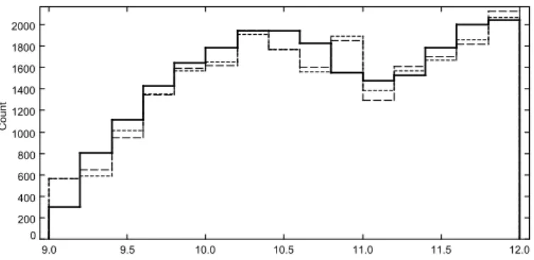
Figure
1
shows the comparison of the I-magnitude
distribu-tion of the selected samples in observadistribu-tions and simuladistribu-tions. The
distribution in I in the simulation is close to the distribution of
the real data. In order to check the distribution in astrophysical
0 200 400 600 800 1000 1200 1400 1600 1800 2000 9.0 9.5 10.0 10.5 11.0 11.5 12.0 Count
Fig. 1.
Distribution in I magnitude of the observed sample (solid line)
of stars with reliable radial velocities and metallicities, and simulated
sample (dashed and dotted line for two independent simulated samples)
for the whole RAVE survey.
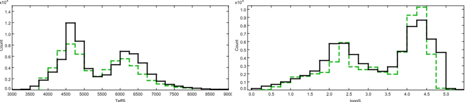
parameters of the whole sample, Fig.
2
presents the histogram
of the distribution in e
ffective temperature and the gravity of the
simulated and observed sample.
In some cases the number of stars with reliable radial
ve-locities and metallicities in RAVE data is on the order of 50
to 150 per field. This implies a significant Poisson noise when
performing comparisons in metallicity bins. Therefore, we used
simulations that have five times the number of observed stars to
decrease the Poisson noise, and we performed eight independent
runs starting from random initial values in order to avoid to be
stacked in local maxima of the likelihood.
3. Basis of the kinematical model
The kinematics of the stars is computed from simple
assump-tions of the relaassump-tions between ages and velocity ellipsoids for
the thin disk and ad hoc empirical values for the thick disk and
the halo, as described below. The kinematics in the bar is more
complex. In another study we use the bar potential to derive the
velocity distributions from test-particle simulations
(Fernández-Trincado et al., in prep.). For the purpose of the present work, the
bar kinematics is not relevant since the bar population does not
reach the RAVE sample in significant numbers. Although the bar
potential can perturb the kinematics of the disk stars in the solar
neighborhood, we here provisionally considered a local
axisym-metric potential. We adopted the usual reference system, with U
toward the Galactic center, V toward rotation, and W toward the
North Galactic Pole.
3.1. Thin disk
The thin-disk kinematics is based on the velocity ellipsoids
with dispersions varying with age, following the study of
Bienaymé et al.
(
1987
). Table
1
gives the assumed age-velocity
dispersion relation used in the previous Besançon Galaxy Model
(
Robin et al. 2003
) following the determination of
Gómez et al.
(
1997
) from the H
ipparcos
sample. The velocity dispersions
increase with age, as expected for a secular evolution from a
circular disk.
Holmberg et al.
(
2009
) proposed velocity
disper-sions slightly higher than
Gómez et al.
(
1997
). RAVE and TGAS
data provide a good opportunity to derive a more accurate
age-velocity dispersion relation. We here considered that the age-velocity
dispersion increases with age following three di
fferent formulae:
1) a third-order polynomial (Eq. (
1
)); 2) the square-root formula
proposed by
Wielen
(
1977
; Eq. (
2
)); 3) the power-law formula
Table 1. Velocity ellipsoid as a function of age for the seven components
of the thin disk in the standard Besançon galaxy model.
Subcomponent
Age range
σ
U
σ
V
σ
W
Gyr
km s
−1
km s
−1
km s
−1
1
0.−0.15
16.7
10.8
6.0
2
0.15−1.
19.8
12.8
8.0
3
1.−2.
27.2
17.6
10.0
4
2.−3.
30.2
19.5
13.2
5
3.−5.
36.7
23.7
15.8
6
5.−7.
43.1
27.8
17.4
7
7.−10.
43.1
27.8
17.5
taken from
Aumer et al.
(
2016
; Eq. (
3
)).
σ
W
= A + B × τ + Cτ
2
,
(1)
σ
W
=
√
α + γ × τ,
(2)
σ
W
= k × τ
β
,
(3)
where τ is the age in Gyr.
Then the velocity dispersion in U and V are defined relative
to σ
W
by the ratios σ
U
/σ
V
and σ
U
/σ
W
, which are free
parame-ters and assumed to be independent of time.
In the fitting process we also considered the vertex deviation,
allowing for two di
fferent angles VD
a
and V D
b
for stars with
ages younger or older than 1 Gyr, respectively.
3.2. Thick disk
The thick-disk velocity ellipsoid su
ffers from uncertainties that
are mainly due to the way that this population is selected in
dif-ferent data sets. The relative continuity (or lack of clear
separa-tion) of the two disk populations, when no elemental abundances
are available, has been the source of misunderstanding and
ap-parent inconsistency between various analyses. With the help of
the alpha-element abundance ratio it can be easier to analyze,
since it has been shown in local samples (
Adibekyan et al. 2013
)
and more distant samples (
Hayden et al. 2014
), among others,
that the thick disk can be better separated from the thin disk
us-ing the [α
/Fe] ratio. However, the abundances in RAVE DR4 are
not accurate enough to clearly distinguish the thick disk from
the thin-disk sequence in the [α
/Fe] versus [Fe/H] plane. After
several tests, we decided to use only [Fe
/H] to separate the
pop-ulations in the present analysis.
According to
Robin et al.
(
2014
), the scale length and scale
height change from the beginning (12 Gyr ago) to the end of
the phase (10 Gyr ago) because of contraction. Hence we expect
that the velocity ellipsoid and rotation velocity show a similar
behavior.
For the present analysis we chose to keep the velocity
disper-sions of the thick disk as free parameters together with its
rota-tion velocity, but we assumed that these parameters are di
fferent
for the two thick-disk episodes, mimicking a time evolution. The
fourth-order dependency on time of the velocity dispersion
ellip-soids takes this into account.
The other populations (halo and bar) are very marginal in the
RAVE survey and will not change the result of the analysis.
3.3. Rotation curve and asymmetric drift
In order to simulate the kinematics of stars at larger distances
from the Sun, we used the rotation curve produced by the mass
0.0 0.2 0.4 0.6 0.8 1.0 1.2 1.4 x10⁴ 3000 3500 4000 4500 5000 5500 6000 6500 7000 7500 8000 8500 9000 TeffS Count 0.0 0.1 0.2 0.3 0.4 0.5 0.6 0.7 0.8 0.9 1.0 x10⁴ 0.0 0.5 1.0 1.5 2.0 2.5 3.0 3.5 4.0 4.5 5.0 loggS Count
Fig. 2.
Distribution in e
ffective temperature (left panel) and gravity (right panel) of the observed sample (solid line) of stars with reliable radial
velocities and metallicities, and simulated sample (dashed line) for the selection |b| > 20
◦
and I < 12.
150 200 250 300 350 2 4 6 8 10 12 14 16 18 20 V (km/s) R (kpc) Caldwell+ (1981) Model 1 Sofue2015 Model 2Fig. 3.
Rotation curve of the mass model, compared with
Caldwell & Ostriker
(
1981
) and
Sofue
(
2015
). The interval between the
two dashed lines indicates the range of Galactocentric distances implied
in the present study.
model. To compute the radial force, we summed the
differ-ent mass compondiffer-ents (stellar populations, interstellar matter,
and dark matter halo) and derived the circular velocity as a
function of Galactocentric radius. In this process described in
Bienaymé et al.
(
1987
), we used observational data either from
Caldwell & Ostriker
(
1981
) or from
Sofue
(
2015
) to constrain
the dark matter halo distribution and the thin-disk ellipsoid axis
ratio. The resulting rotation curves are presented in Fig.
3
. There
is a significant di
fference between the two rotation curves, but
at the solar position, their slopes are very similar. As we show
below, they result in a similar fit to RAVE
+TGAS data because
these data mainly constrain the velocity dispersions, the slope of
the rotation curve, and the asymmetric drifts, but set only weak
constraints on the amplitude of the rotation curve itself.
The asymmetric drift was then computed to take the change
of the circular velocity as a function of age and distance from the
plane with regard to the rotation curve into account. It depends
on the velocity dispersion ratio, on density and kinematic
gra-dients, and on the di
fference of the radial force as a function of
R
gal
and z
gal
.
In the past we used the simplified formula of the
asymmet-ric drift proposed by
Binney & Tremaine
(
2008
), which is valid
in the Galactic plane. In order to have a more consistent
expres-sion of the asymmetric drift as a function of distance from the
plane, we made use of the gravitational potential inferred by
the mass distribution of the BGM.
Bienaymé et al.
(
2015
)
pro-posed distribution functions based on a Stäckel approximation
of the BGM potential, for which it is possible to compute a
third integral of motion. An approximate fit of the variations of
the asymmetric drift with (R
gal
, z
gal
) Galactocentric coordinates
was computed and used in the kinematical modeling. This
ap-proximation is valid in the range 2 kpc < R
gal
< 16 kpc and
−6 kpc < z
gal
< 6 kpc and was shown to be a very good
approx-imation, as the K
z
is reproduced at better than 1%. The resulting
rotational lag of di
fferent thin- and thick-disk subcomponents are
shown to strongly depend on R
gal
and z
gal
. These dependencies
are presented in Fig.
4
.
3.4. Solar velocities
There have been a number of studies that tried to measure the
peculiar velocities of the Sun. The U and W velocities are
rel-atively well known and have been constrained at a level of
1−2 km s
−1
. This is not the case for the V velocity, which is
uncertain because it is di
fficult to distinguish it from the mean
circular motion of the LSR. Hence, while in the past it was
admitted to be about 5−6 km s
−1
(see, i.e.,
Dehnen & Binney
1998
), more recent studies found much higher values. For
exam-ple,
Schönrich et al.
(
2010
) found about 12 km s
−1
from a
sub-set of the Geneva-Copenhagen Survey (GCS), while
Bovy et al.
(
2012
) from the APOGEE first data release (
Ahn et al. 2014
)
found an even higher value of 26 ± 3 km s
−1
). These values
are not independent of the tracer selection, mostly K giants in
the case of
Bovy et al.
(
2012
) and mostly dwarfs in the case of
Schönrich et al.
(
2010
). The values also significantly depend on
the rotation curve that is assumed and on the distance between
the Sun and the Galactic center. This is why in our analysis the
solar motion is a free parameter that can be influenced by other
parameters and by the way the asymmetric drift is modeled.
4. Setting up the MCMC
This study uses an ABC-MCMC code based on a
Metropolis-Hasting sampling, as described in
Robin et al.
(
2014
). Table
2
shows the set of model parameters to fit and their respective
range. To estimate the goodness-of-fit for each model, we
di-rectly compared histograms of radial velocity and proper
mo-tions between the model and the data. The bin steps in radial
velocity and proper motions are 5 km s
−1
and 5 mas
/yr,
re-spectively. To improve the sensitivity of the analysis, however,
we separated stars using their metallicity and temperature. The
metallicity rather than α abundances was used because the
ac-curacy in α in the RAVE survey does not allow us to separate
the thin disk well from the thick-disk sequences, and we expect
that the metallicity is more accurate. Moreover, to separate the
young thick disk from the old thick disk, the metallicity is more
0
20
40
60
80
100
120
140
160
0
1
2
3
4
5
6
Vlag km/s
Zgal (kpc)
0
10
20
30
40
50
60
70
80
90
100
2
4
6
8
10
12
Vlag km/s
Rgal (kpc)
Fig. 4.
Asymmetric drift computed from the Stäckel approximation of the BGM for subcomponents 2 to 7 (thin disk, with increasing ages plotted
in solid red, long dashed green, short dashed blue, dotted magenta, dashed yellow and cyan), and for the young (dot-dashed black) and old
(dot-dot-dashed red) thick disks. Left panel: as a function of R
gal
for z
gal
= 0; right panel: as a function of z
gal
for R
= R
.
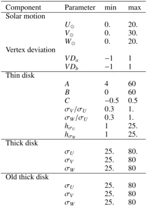
Table 2. Set of parameters and range used in the ABC-MCMC process.
Component
Parameter
min
max
Solar motion
U
0.
20.
V
0.
30.
W
0.
20.
Vertex deviation
V D
a
−1
1
V D
b
−1
1
Thin disk
A
4
60
B
0
60
C
−0.5
0.5
σ
V
/σ
U
0.3
1.
σ
W
/σ
U
0.3
1.
h
σ
U1
25.
h
σ
W1
25.
Thick disk
σ
U
25.
80.
σ
V
25.
80
σ
W
25.
80
Old thick disk
σ
U
25.
80
σ
V
25.
80
σ
W
25.
80
Notes. Units are km s
−1
for velocities and radian for the vertex
devia-tion. Thin-disk parameters A–C are the coefficients of the formula
de-scribing the evolution of σ
W
with time (see text). The vertex deviation
is for ages younger (V D
a
) and older (V D
b
) than 1 Gyr, and the scale
lengths are given in kpc. Velocities and velocity dispersions are all given
in km s
−1
.
efficient than the α abundances, and it also separate the
metal-rich thin disk better from the normal thin disk.
We made use of four metallicity bins, where lower
metallic-ities are dominated by the thick disk and higher metallicmetallic-ities by
the thin disk. The minimum metallicity is −1.2 and the width of
each bin is 0.4 dex. To separate dwarfs from giants, we cut at a
temperature of 5300 K, considering that cooler stars are mainly
giants, while hotter stars are mainly dwarfs. However, we did not
explicitly assume that they are dwarfs or giants in the analysis.
We merely considered these two bins and computed histograms
of velocities and likelihoods for these two bins separately in both
data and simulations to enhance the e
fficiency of the fit of the
parameters depending on ages. For the proper motions we used
projections on Galactic coordinates, µ
∗
l
= cos(b) × µ
l
and µ
b
,
but for the South Galactic cap it is more interesting to project
the proper motions parallel to the U and V vectors, U pointing
toward the Galactic center, and V toward rotation. This
facili-tates the interpretation of the histogram comparisons because it
clearly shows the skewness of the V distribution that is due to
the asymmetric drift.
The likelihoods were computed separately for 11 regions
of the sky, corresponding to different latitudes and quadrants
in longitudes. The likelihood is based on the formula given in
Bienaymé et al.
(
1987
) for a Poisson statistics. Then, to
inter-compare di
fferent models with a different number of free
param-eters, we computed the Bayesian information criterion (BIC)
fol-lowing
Schwarz
(
1978
), which penalizes models with more free
parameters (Eq. (
4
)),
BIC
= −2. × Lr + k × ln(n),
(4)
where Lr is the likelihood, k is the number of parameters, and n
the number of observations used in the likelihood computation.
At the end of the process, we considered the last third of
each Markov chain, containing 200 000 iterations each, for eight
independent runs of the MCMC and computed the mean and
dis-persion for each fitted parameter.
5. Results
The values of the fitted parameters are given in Tables
3
–
5
for
the age-velocity dispersion as a fourth-order polynomial, square
root formula, and power-law formula, respectively. The
veloc-ity dispersions for the old thick disk are noticeably larger than
the dispersion of the young thick disk, as expected from their
respective scale heights. This confirms the collapse with time
during the thick-disk phase and the probable contraction from a
larger thick disk with slower rotation in the past toward a smaller
and more concentrated thick disk with faster rotation later on.
The solar velocities are also well constrained by this
analy-sis, and we find mean motions in good agreement with previous
Table 3. Best values of fitted parameters obtained by the mean of the
last third of eight independent chains and standard deviation assuming
Caldwell & Ostriker
(
1981
) and
Sofue
(
2015
) rotation curves.
Parameter
Caldwell
Sofue
Solar motion
U
12.75 ± 1.26
11.88 ± 1.38
V
0.93 ± 0.30
0.91 ± 0.26
W
7.10 ± 0.16
7.07 ± 0.16
Vertex deviation
V D
a
−0.0439 ± 0.0375
−0.0618 ± 0.0218
V D
b
−0.0144 ± 0.0122
−0.0048 ± 0.0108
Thin disk
A
5.69 ± 0.37
5.69 ± 0.41
B
2.48 ± 0.30
2.33 ± 0.28
C
−0.0966 ± 0.0404
−0.0774 ± 0.0362
σ
V
/σ
U
0.57 ± 0.03
0.58 ± 0.03
σ
W
/σ
U
0.46 ± 0.03
0.46 ± 0.02
h
σ
U13 176. ± 6908.
9534. ± 3982.
h
σ
W15 919. ± 8609.
10 414. ± 6299.
Thick disk
σ
U
40.02 ± 1.74
41.58 ± 1.51
σ
V
31.86 ± 1.55
30.95 ± 1.50
σ
W
27.89 ± 1.26
27.02 ± 1.00
Old thick disk
σ
U
75.64 ± 8.58
79.64 ± 7.96
σ
V
55.41 ± 8.74
57.55 ± 8.51
σ
W
66.43 ± 3.95
62.15 ± 6.62
Lr
−5384. ± 38.
−5378. ± 155.
BIC
10 861. ± 76.
10 851. ± 161.
Notes. Units are km s
−1
for velocities, pc for the scale lengths, and
radi-ans for the vertex deviation, which is given for stars younger than 1 Gyr
(V D
a
) and older than 1 Gyr (V D
b
). A, B, and C are the coefficients of
the polynomial describing the variation of σ
W
with age in Gyr (Eq. (
1
)).
The BIC is computed from Eq. (
4
).
studies for U and W velocities. For the case of the circular
ve-locity, we obtained a lower value than has been found in many
other studies. This is discussed in the next section.
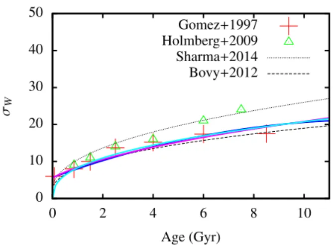
The thin-disk di
ffusion with time is also constrained to
be close to the values obtained by
Gómez et al.
(
1997
) from
H
ipparcos
data. Figure
5
shows the comparison between the
results of our fits with the three assumed formulas and data from
Holmberg et al.
(
2009
) and
Gómez et al.
(
1997
). The agreement
is good for the young ages with both determinations but is
closer to
Gómez et al.
(
1997
) for the older stars. We also
over-plot the velocity dispersion as a function of time obtained by
Sharma et al.
(
2014
) and by
Bovy et al.
(
2012
) for the further
discussion.
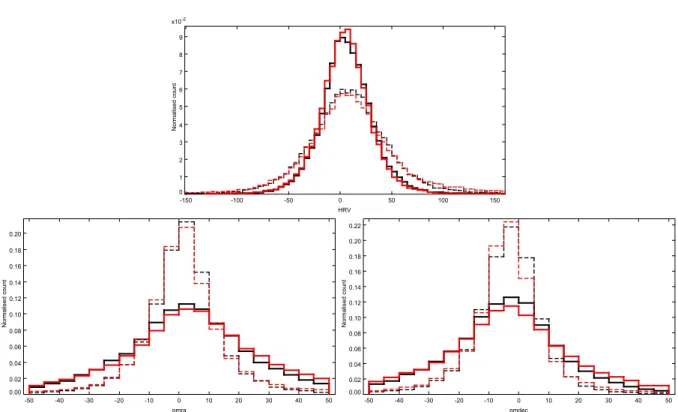
To visually evaluate the agreement between model and data,
we show in Fig.
6
histograms for cool stars (T
e
ff
< 5300 K)
and hot stars (T
e
ff
> 5300 K) of radial velocities and proper
motions. We clearly see that cool stars present larger velocity
dispersions (seen from radial velocity histograms), although in
proper motions their dispersions are smaller because of the
dis-tance e
ffect in these mostly giant stars.
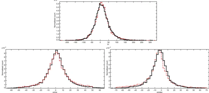
Histograms of radial velocity and proper motions by
metal-licity bins are shown in Fig.
7
for the metallicity range −1.2 <
[M/H] < −0.8 (dominated by the old thick disk), in Fig.
8
for
−0.8 < [M/H] < −0.4 (dominated by the young thick disk),
in Fig.
9
for −0.4 < [M/H] < −0 (mainly thin disk), and in
Fig.
10
for −0.4 < [M/H] < 0.4 (metal-rich thin disk). We note
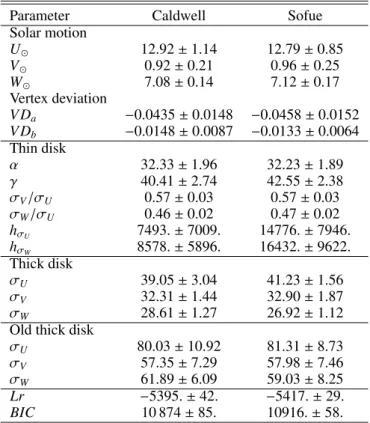
Table 4. Same as Table
3
, but here α and γ are the parameters of the
square-root function of the velocity dispersion as a function of age
in Gyr (Eq. (
2
)).
Parameter
Caldwell
Sofue
Solar motion
U
12.92 ± 1.14
12.79 ± 0.85
V
0.92 ± 0.21
0.96 ± 0.25
W
7.08 ± 0.14
7.12 ± 0.17
Vertex deviation
V D
a
−0.0435 ± 0.0148
−0.0458 ± 0.0152
V D
b
−0.0148 ± 0.0087
−0.0133 ± 0.0064
Thin disk
α
32.33 ± 1.96
32.23 ± 1.89
γ
40.41 ± 2.74
42.55 ± 2.38
σ
V
/σ
U
0.57 ± 0.03
0.57 ± 0.03
σ
W
/σ
U
0.46 ± 0.02
0.47 ± 0.02
h
σ
U7493. ± 7009.
14776. ± 7946.
h
σ
W8578. ± 5896.
16432. ± 9622.
Thick disk
σ
U
39.05 ± 3.04
41.23 ± 1.56
σ
V
32.31 ± 1.44
32.90 ± 1.87
σ
W
28.61 ± 1.27
26.92 ± 1.12
Old thick disk
σ
U
80.03 ± 10.92
81.31 ± 8.73
σ
V
57.35 ± 7.29
57.98 ± 7.46
σ
W
61.89 ± 6.09
59.03 ± 8.25
Lr
−5395. ± 42.
−5417. ± 29.
BIC
10 874 ± 85.
10916. ± 58.
Table 5. Same as Table
3
but where k and β are the parameters of the
power law function of the velocity dispersion as a function of age in Gyr
(Eq. (
3
)).
Parameter
Caldwell
Sofue
Solar motion
U
13.00 ± 1.02
13.12 ± 1.47
V
0.94 ± 0.23
0.92 ± 0.29
W
7.01 ± 0.15
7.03 ± 0.18
Vertex deviation
V D
a
−0.0325 ± 0.0131
−0.0388 ± 0.0126
V D
b
−0.0173 ± 0.0075
−0.0167 ± 0. 0111
Thin disk
k
8.30 ± 0.19
8.26 ± 0.22
β
0.40 ± 0.02
0.40 ± 0.02
σ
V
/σ
U
0.54 ± 0.02
0.57 ± 0.03
σ
W
/σ
U
0.46 ± 0.02
0.47 ± 0.02
h
σ
U19 430. ± 3948.
13009. ± 8856.
h
σ
W11 813. ± 8010.
10473. ± 7058.
Thick disk
σ
U
40.36 ± 2.00
42.18 ± 2.05
σ
V
32.85 ± 1.44
32.26 ± 2.06
σ
W
27.03 ± 1.20
26.90 ± 1.10
Old thick disk
σ
U
80.30 ± 10.32
75.87 ± 5.52
σ
V
57.81 ± 6.35
53.93 ± 5.87
σ
W
62.24 ± 5.25
66.22 ± 3.23
Lr
−5429 ± 32
−5420. ± 31.
BIC
10 942 ± 65
10 923. ± 62.
that the fit to each individual population is good, with a higher
dispersion for the old thick disk than for the young thick disk,
as expected and seen in the dispersion in Table 3. For metal-rich
0
10
20
30
40
50
0
2
4
6
8
10
σ
W
Age (Gyr)
Gomez+1997
Holmberg+2009
Sharma+2014
Bovy+2012
Fig. 5.
Evolution of the vertical velocity dispersion of the thin disk with
age. The solid lines show the best-fit solutions for the three different
formulae (fit 1: blue, fit 2: magenta, fit 3: cyan, see text), while the
symbols indicate the
Gómez et al.
(
1997
) values from H
ipparcos
(red
plus) and
Holmberg et al.
(
2009
; green triangles). The black dotted line
is the relation from
Sharma et al.
(
2014
), while the black dashed line is
the relation from
Bovy et al.
(
2012
).
stars, the proper motion in declination shows a slight shift, which
could be due to the vertex deviation, which is expected to be
higher in these (in the mean) younger stars. We consider to
im-plement a spiral arm model in the future to investigate and solve
this problem.
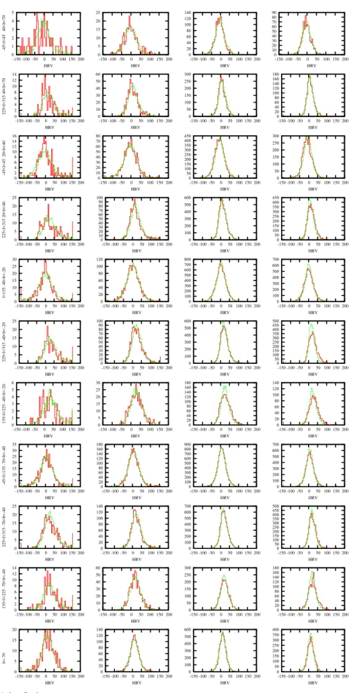
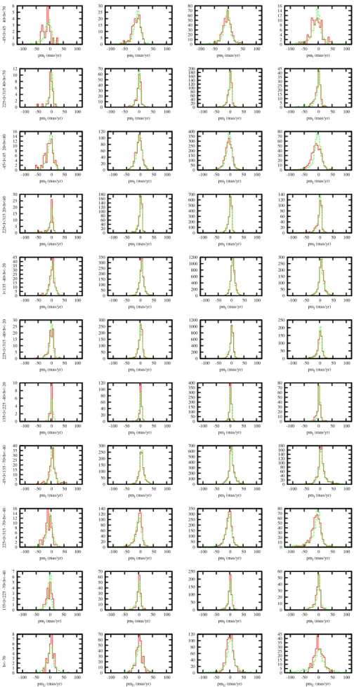
In order to have a complete view of the agreement of the
model in different regions of the sky, histograms of RAVE radial
velocities and TGAS proper motions in the 11 sky regions used
are presented in Appendix A, where the data are plotted as solid
lines and the model as dashed lines. Figures
A.1
,
A.3
, and
A.5
show histograms for cool stars, while Figs.
A.2
,
A.4
, and
A.6
present similar plots for hot stars. In each figure, the columns
indicate the metallicity range we used, from ]−1.2; −0.8] on the
left to [0; 0.4] on the right. This shows that the old (metal-weak)
thick disk dominates in the first column, the main thick disk in
the second column, the main thin disk in the third column, and
the metal-rich thin disk dominates in the fourth column.
The histograms show very good agreements between the
model and the data in nearly all cases. There is noticeable
Pois-son noise in the old thick disk (first column) in many cases,
which explains why the uncertainties on the parameters of this
population are sensitively larger than for the thin (third and
fourth columns) and young thick disks (second column). The
hotter stars show significantly smaller dispersions than cooler
stars in proper motions, which is mainly because the giants
(cooler) are at larger distances in the mean. We also note the
strong skewness of the distributions in many cases, which
ex-plains the necessity to fit the whole histograms and not only the
mean and standard deviation of each parameter.
Although the global fits are very good, there are a few
no-ticeable di
fferences in some fields that are probably due to some
substructures, such as streams, associations, or clusters. It is also
possible that our vertex deviation does not represent the real one
well and needs to be better modeled, for example, with a spiral
arm model. The regions that present systematic deviations with
the TGAS proper motions are the South Galactic cap (shift and
dispersion in µ
U
and µ
V
), although the radial velocity dispersion
is well reproduced. Even though TGAS is much more
homoge-neous and well behaved than previous astrometric surveys, it is
not completely free of systematics, as shown by
Arenou et al.
(
2017
), especially because of the scanning law and the limited
number of observations included in this first release. Future Gaia
releases will allow us to solve this problem. Toward the Galactic
center at intermediate latitudes (−45 < l < 45, 25 < b < 40),
there is also a significant disagreement in µ
l
for hot stars.
How-ever, the fit is nearly perfect in µ
b
for all types of stars, cool and
hot, and any metallicities. Proper motion histograms of hot stars
also agree very well in all directions, but for the stars that are at
larger distances, it might be harder to distinguish significant
de-viations from an axisymmetric model. The radial velocities from
RAVE are very well reproduced by the model, especially for hot
stars at all metallicities and in all directions. For low-metallicity
cool stars, the histograms are noisy because of the small
num-ber of stars, but the histograms for high-metallicity bins are well
reproduced in all regions.
6. Discussion
Compared with previous RAVE analysis, we have used di
ffer-ent hypotheses that are improvemffer-ents and probably give more
reliable results. First, we use an improved asymmetric drift that
explicitly depends on R
gal
and z
gal
and on age and is consistent
with the Galactic potential. Second, we use the metallicity to
help distinguish the thin from the thick disk, and we separately
consider temperature bins dominated by dwarfs and giants,
re-spectively. Third, we explicitly take the selection bias of the data
into account and compare the model simulations in the space
of observables. Fourth, we explore the full parameter space and
also determine the radial velocity dispersion gradients (or
kine-matical scale length).
Using this method, we obtain reliable results for the various
tested parameters that describe the kinematics of stellar
popula-tions, as discussed below. We separately discuss the V
compo-nent of the solar motion, which is related to the circular velocity
of the LSR, to the rotation curve, and to the asymmetric drift.
6.1. U and W components of the solar motion
We obtained the following values for the solar motion
U
= 13.2 ± 1.3 km s
−1
and W
= 7.1 ± 0.2 km s
−1
.
For the U
velocity, our value agrees well with previous
results (
Aumer & Binney 2009
: 9.96 ± 0.33;
Schönrich et al.
2010
: 11.1 ± 0.7;
Co¸skunoˇglu et al. 2011
: 8.5 ± 0.4 km s
−1
;
Pasetto et al. 2012a
: 9.87 ± 0.37 km s
−1
;
Karaali et al. 2014
:
10 km s
−1
;
Sharma et al. 2014
: 11.45 ± 0.1;
Bobylev & Bajkova
2015
: 6.0;
Bobylev & Bajkova 2016
: 9.12). The error bars do not
generally take into account the systematics that are due to the
model that was used.
Bobylev & Bajkova
(
2016
) noted a slight
degeneracy between U and V solar motion that is due to the
por-tion of sky covered by RAVE.
The vertical solar motion is more reliably determined in most
of the studies, with consistent values on the order of 7±1 km s
−1
.
We confirm this value.
6.2. Thin-disk velocity ellipsoid and gradients
Williams et al.
(
2013
) restricted their analysis to red clump
stars in their study of the RAVE survey. They studied in
par-ticular the di
fferences between north and south, looking for
axisymmetry, which we did not include. Evidence of
non-axisymmetries has previously been pointed out by
Siebert et al.
(
2011a
) in the analysis of RAVE third data release (
Siebert et al.
2011b
). We dedicate such an analysis to a future paper. In
their Fig. 8,
Williams et al.
(
2013
) found that the asymmetric
drift varies with z
gal
by about 40 km s
−1
between z
gal
= 0 and
0 1 2 3 4 5 6 7 8 9 x10⁻² -150 -100 -50 0 50 100 150 HRV Normalised count 0.00 0.02 0.04 0.06 0.08 0.10 0.12 0.14 0.16 0.18 0.20 -50 -40 -30 -20 -10 0 10 20 30 40 50 pmra Normalised count 0.00 0.02 0.04 0.06 0.08 0.10 0.12 0.14 0.16 0.18 0.20 0.22 -50 -40 -30 -20 -10 0 10 20 30 40 50 pmdec Normalised count
Fig. 6.
Histograms of RAVE radial velocity distributions (top panel) and TGAS proper motions (bottom panels: left: proper motion along the right
ascension; right: along the declination) for hot (solid lines) and cool (dashed lines) stars. Data are shown as black lines, and the best-fit model is
shown as red lines.
0.0 0.5 1.0 1.5 2.0 2.5 3.0 3.5 4.0 x10⁻² -200 -150 -100 -50 0 50 100 150 200 250 300 Vr Normalised count 0 1 2 3 4 5 6 7 8 9 x10⁻² -60 -50 -40 -30 -20 -10 0 10 20 30 40 50 60 pmra Normalised count 0.00 0.01 0.02 0.03 0.04 0.05 0.06 0.07 0.08 0.09 0.10 0.11 -70 -60 -50 -40 -30 -20 -10 0 10 20 30 40 50 60 70 pmdec Normalised count
Fig. 7.
Histograms of RAVE radial velocity distributions (top panel) and TGAS proper motions (bottom panels: left: proper motion along the right
ascension; right: along the declination) for the metallicity bin −1.2 to −0.8 dex, dominated by the old thick disk. Data are shown as black solid
lines, and the best-fit model is shown as red dashed lines.
z
gal
= 2 kpc, which is in good agreement with our model. The lag
in V
φ
at the z
gal
= 0 is approximately constant with R
gal
, which
also agrees with our results. These studies did not investigate the
dependency of the velocity ellipsoid on age, as we did.
In their study of a RAVE internal data release, intermediate
between DR3 and DR4,
Pasetto et al.
(
2012b
) performed a
de-tailed analysis of the velocity ellipsoid and cross-terms of the
velocity dispersion and their variation with R
gal
and z
gal
.
Simi-larly to our study, they did not find any evidence of variations
with R
gal
, most probably because the RAVE sample is not deep
enough to reach regions where the sensitivity to R
gal
can be
significant. In this study, the mean velocity dispersions for the
thin-disk component were found to be (26, 20, and 16) along the
U, V, W components, respectively, which is in good agreement
with our values because we studied its variation with age, while
they did not. Their values are close to the values for the old thin
disk.
Sharma et al.
(
2014
) investigated the disk kinematics from
GCS and RAVE data analysis with an MCMC method, but with
considerable di
fferences with our results in the assumptions and
in the fitting method. They used parameters from an older stellar
population model (
Robin et al. 2003
) introduced in the Galaxia
0.0 0.5 1.0 1.5 2.0 2.5 3.0 3.5 4.0 4.5 5.0 5.5 x10⁻² -200 -150 -100 -50 0 50 100 150 200 250 300 Vr Normalised count 0 1 2 3 4 5 6 7 8 9 x10⁻² -60 -50 -40 -30 -20 -10 0 10 20 30 40 50 60 pmra Normalised count 0 1 2 3 4 5 6 7 8 9 x10⁻² -70 -60 -50 -40 -30 -20 -10 0 10 20 30 40 50 60 70 pmdec Normalised count
Fig. 8.
Same as Fig.
7
for the metallicity bin −0.8 to −0.4 dex, which is dominated by the main thick disk.
0 1 2 3 4 5 6 7 8 x10⁻² -200 -150 -100 -50 0 50 100 150 200 250 300 Vr Normalised count 0 1 2 3 4 5 6 7 8 9 x10⁻² -60 -50 -40 -30 -20 -10 0 10 20 30 40 50 60 pmra Normalised count 0 1 2 3 4 5 6 7 8 9 x10⁻² -70 -60 -50 -40 -30 -20 -10 0 10 20 30 40 50 60 70 pmdec Normalised count
Fig. 9.
Same as Fig.
7
for the metallicity bin −0.4 to 0 dex, which is dominated by the main thin disk.
0 1 2 3 4 5 6 7 8 9 x10⁻² -200 -150 -100 -50 0 50 100 150 200 250 300 Vr Normalised count 0 1 2 3 4 5 6 7 8 9 x10⁻² -60 -50 -40 -30 -20 -10 0 10 20 30 40 50 60 pmra Normalised count 0 1 2 3 4 5 6 7 x10⁻² -70 -60 -50 -40 -30 -20 -10 0 10 20 30 40 50 60 70 pmdec Normalised count