Optimization of a 4th generation CMB space mission

HAL Id: tel-02019119

https://tel.archives-ouvertes.fr/tel-02019119v2

Submitted on 18 Apr 2019

HAL is a multi-disciplinary open access archive for the deposit and dissemination of sci-entific research documents, whether they are pub-lished or not. The documents may come from teaching and research institutions in France or abroad, or from public or private research centers.

L’archive ouverte pluridisciplinaire HAL, est destinée au dépôt et à la diffusion de documents scientifiques de niveau recherche, publiés ou non, émanant des établissements d’enseignement et de recherche français ou étrangers, des laboratoires publics ou privés.

Ranajoy Banerji

To cite this version:

Ranajoy Banerji. Optimization of a 4th generation CMB space mission. Physics [physics]. Université Sorbonne Paris Cité, 2017. English. �NNT : 2017USPCC199�. �tel-02019119v2�

UNIVERSITÉ SORBONNE PARIS CITÉ

Thèse préparée

à L’UNIVERSITÉ PARIS DIDEROT

École doctorale STEP’UP – ED N

◦

₅₆₀

Laboratoire Astroparticule et Cosmologie

Optimisation d’une mission spatiale

CMB de 4

eme

génération

par

Ranajoy Banerji

présentée et soutenue publiquement le

21 septembre 2017

Thèse de doctorat de Science de la Terre et de l’environnement

dirigée par Jacques Delabrouille

devant un jury composé de :

Jacques Delabrouille Directeur de thèse

Directeur de recherche CNRS-IN2P3, APC, Paris-VII Stavros Katsanevas Président

Professeur APC, Paris-VII Karim Benabed Rapporteur Directeur de recherche IAP, UPMC Anthony Challinor Rapporteur

Reader Institute of Astronomy, University of Cambridge Delphine Hardin Membre

Professeur LPNHE, UPMC Nicolas Ponthieu Membre

A

BSTRACT

T

he Cosmic Microwave Background radiation is a rich and clean source of Cosmologicalinformation. Study of the CMB over the past few decades has led to the establishment of a “Standard Model” for Cosmology and constrained many of its principal parameters. It has also transformed the field into a highly data-driven domain.

Currently, Inflation is the leading paradigm describing the earliest moments of our Universe. It predicts the generation of primordial matter density fluctuations and gravitational waves. The CMB polarisation carries the signature of these gravitational waves in the form of primordial “B-modes”. A future generation of CMB polarisation space mission is well suited to observe

this signature of Inflation.

This thesis focuses on optimising a future CMB space mission that will observe the B-mode signal for reaching a sensitivity ofr = 0.001. Specifically, I study the optimisation of the scanning strategy and the impact of systematics on the quality of polarisation measurement.

R

ÉSUMÉ

L

e rayonnement du Fond Diffus Cosmologique est une source riche et propre d’informationscosmologiques. L’ étude du CMB au cours des dernières décennies a conduit à la mise en place d’un modèle standard pour la cosmologie et a permis de mesurer précisément ses principaux paramètres. Il a également transformé le domaine, en le basant davantage sur les données observationnelles et les approches numériques et statistiques.

A l’heure actuelle, l’inflation est le principal paradigme décrivant les premiers moments de notre Univers. Elle prédit la génération de fluctuations de la densité de matière primordiale et des ondes gravitationnelles. Le signal de polarisation du CMB porte la signature de ces ondes gravitationnelles sous la forme de modes-B primordiaux. Une future génération de missions spatiale d’observation de la polarisation du CMB est bien adaptée à l’observation de cette signature de l’inflation.

Cette thèse se concentre sur l’optimisation d’une future mission spatiale CMB qui observera le signal en modes-B pour atteindre une sensibilité de r = 0,001. Plus précisément, j’étudie la stratégie d’observation et l’impact des effets systématiques sur la qualité de la mesure de polarisation.

D

EDICATION AND ACKNOWLEDGEMENTS

F

irst and foremost to thank is my PhD supervisor who took me on when I hardly knewanything about CMB observation. He kept feeding me interesting ideas and provided me space to let them grow into the work I present here. Collaborating with others at APC, especially Guillaume, helped me develop my work faster and introduced me to new ideas. APC has been a great place to work and I wish to thank anyone else who I have come across here over the years.

Among the students at APC my first shout goes out to Pierros for being a great friend. To all the others who have been occupants of 427B and 312B over the years especially Cyrille, Alessandro, Thuong and Mikhail, my appreciation of your friendship. The help I received from Julien and Davide helped me overcome several of my deficiencies regarding the CMB and computing. The coffee sessions with Dhiraj every afternoon was something I looked forward to and enjoyed the interesting discussions which ranged from physics to politics to movies. For the constant supply of great coffee a special thanks to Ken.

To all my friends and acquaintances, Paris would not have been the same without you. Special thanks to Bitan, Ayan and Shantanu for being wonderful and supportive friends. It goes without mentioning that my life would have been different without my best friend Debashmita, whose support and friendship is what got me through life on several occasions.

Last but not the least, my parents, who have been supportive of everything I have done in life and allowed my to pursue my dreams, be it music or physics.

T

ABLE OF

C

ONTENTS

Page

List of Tables xi

List of Figures xiii

1 The Cosmic Microwave Background and Inflation 1

1.1 The Expanding Universe . . . 2

1.1.1 The Friedmann-Robertson-Walker Metric . . . 2

1.1.2 Distances, Redshifts and Horizons . . . 3

1.1.3 Dynamics of the FRW Universe . . . 4

1.2 Thermal History of the Universe and Recombination . . . 6

1.3 Inflation . . . 9

1.3.1 Flatness and Horizon Problem . . . 9

1.3.2 Inflation as a Solution to the Flatness and Horizon Problem . . . 10

1.3.3 Mechanism of Inflation . . . 11

1.3.4 Slow-Roll Inflation . . . 12

1.3.5 Production of Initial Perturbations and its Statistics . . . 14

1.4 Imprints on the CMB : Anisotropies . . . 17

1.4.1 Primary Temperature Anisotropies . . . 17

1.5 Polarisation of the CMB . . . 20

1.5.1 Representation of Polarisation . . . 21

1.5.2 Thomson Scattering of Photons . . . 22

1.5.3 Sources of Quadrupole . . . 23

1.6 Late time Cosmology with the CMB . . . 23

1.6.1 Weak gravitational lensing . . . 24

1.6.2 Reionisation . . . 27

1.6.3 Sunyaev-Zeldovich effect . . . 28

1.7 Current Status of Power Spectrum Observation . . . 28

1.7.1 Limit on power spectrum estimation . . . 31

2 Motivation for a CMB Space Mission 35 2.1 The Science Case . . . 36

2.2 Proposed Space Missions . . . 37

2.2.1 CORE . . . 37

2.2.2 LiteBIRD . . . 39

2.3 Practical Advantages of Space . . . 40

3 Scan Strategy 43

3.1 The CORE scan strategy . . . 44

3.2 Scan Parameters . . . 44

3.3 Classification of Scan Strategies . . . 47

3.4 Example Scan Strategies . . . 49

3.5 Sky Coverage and Cross-Linking . . . 50

3.6 Polarisation Reconstruction and Sensitivity . . . 52

3.7 Summary and Discussion . . . 58

4 Systematics Correction Map Making 59 4.1 Known Systematics in Past and Current Experiments . . . 60

4.2 Map Making . . . 61

4.2.1 Ideal Configuration . . . 63

4.3 Signal Leakage due to Non-Idealities and Signal Mismatch . . . 64

4.4 Modelling the Systematic Effects for Pairs . . . 65

4.4.1 Polarisation Misalignment . . . 66

4.4.2 First Order in Leakage Terms . . . 67

4.5 The Leakage as a Nuisance Term . . . 67

4.6 Developing the Regression Algorithm . . . 68

4.6.1 The Estimators . . . 68

4.6.2 Properties of the Estimators . . . 69

4.6.3 Implementing the Algorithm . . . 71

4.7 Summary and Discussion . . . 71

5 The Simulation Code 73 5.1 General Outline . . . 74

5.2 Data Distribution Model . . . 75

5.3 Real Space Beam Convolution . . . 76

5.4 Summary and Discussion . . . 82

6 Bandpass Mismatch 83 6.1 Modelling the Signal . . . 83

6.2 Multi-Detector Maps and Projection of the Leakage . . . 85

6.3 Single-Detector Map-Making . . . 93

6.4 Correction Model for Detector Pairs . . . 94

6.5 Validation of the Correction Algorithm . . . 95

6.6 Correction for Multiple Detectors . . . 97

6.7 Correcting for Multiple Sources . . . 100

6.8 Summary and Discussion . . . 103

7 Beam Asymmetry and Mismatch 105 7.1 Modelling the Signal, and Correcting Method . . . 106

7.2 Results for Elliptical Beams . . . 108

7.3 Simulated Beams for the CORE Proposal . . . 112

7.4 Summary and Discussion . . . 115

TABLE OF CONTENTS

L

IST OF

T

ABLES

TABLE Page

1.1 Evolution of components . . . 5 3.1 Scan configurations . . . 49 4.1 Types of Systematics . . . 60 6.1 Configuration of the focal-plane detectors used in the bandpass mismatch simulation 88 6.2 Comparison of badpass parameter to measured template amplitude in the noiseless

timestream case . . . 99 6.3 Comparison of expected to measured template amplitude for bandpass leakage in

the noisy timestream case . . . 99 6.4 Estimation of bandpass leakage parameter for multiple templates . . . 102

L

IST OF

F

IGURES

FIGURE Page

1.1 Estimates of the curvature, dark energy and matter content from Planck . . . 6

1.2 Thermal history of the Universe . . . 7

1.3 Electron fraction at Recombination . . . 8

1.4 Comoving Hubble radius during Inflation . . . 10

1.5 Constraints on Inflationary parameters . . . 16

1.6 Contributions to the temperature power spectrum . . . 20

1.7 E and B mode pattern . . . 24

1.8 Lensing power spectra current measurements . . . 26

1.9 Results on neutrino mass and Neff . . . 27

1.10 Recent measurement of CMB TT power spectrum . . . 29

1.11 Recent measurement of CMB TE and EE power spectra . . . 30

1.12 Recent measurement of CMB BB spectrum . . . 31

1.13 Effect of Beam . . . 32

1.14 Effect of Noise . . . 33

1.15 Contamination due to galaxy . . . 34

2.1 CORE conceptual design . . . 38

2.2 LiteBIRD design . . . 39

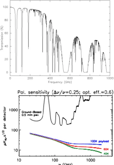
2.3 Atmospheric Transmission and sensitivity . . . 41

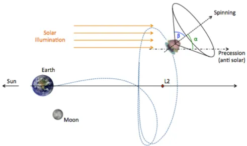
3.1 The CORE instrument orbit at the(L2). . . 44

3.2 The CORE instrument in the instrument reference frame . . . 45

3.3 The two cross-linking scenarios . . . 47

3.4 Cross linking patterns on the hitmap . . . 48

3.5 Comparison of evolution of Hitmap . . . 51

3.6 Evolution of the diagonal terms in the covariance matrix . . . 53

3.7 Evolution of the off-diagonal terms in the covariance matrix . . . 54

3.8 Polarisation sensitivity maps . . . 56

3.9 Polarisation sensitivity cumulative histogram . . . 57

3.10 Polarisation sensitivity histogram . . . 58

5.1 The data distribution model . . . 76

5.2 Movement of beam in the focal plane . . . 78

5.3 Convolution using a real space beam map . . . 78

5.4 Smoothing of the signal with a real space beam convolution . . . 79

5.5 Comparison of maps due to real space beam convolution . . . 80

6.1 Projection of the bandpass leakage signal . . . 89

6.2 Leakage spectra level due to different pairs and combinations . . . 90

6.3 Effect of rotation of polariser on bandpass leakage . . . 91

6.4 BB leakage config comparison for single pair . . . 92

6.5 Comparing noise spectra for single detectors . . . 93

6.6 Bandpass correction using a perfect template . . . 96

6.7 Galactic mask . . . 97

6.8 BB residual leakage comparison for pair combinations . . . 98

6.9 Bandpass parameter estimation . . . 100

6.10 Synchrotron leakage comparison . . . 101

6.11 Multi template banspass leakage correction . . . 102

7.1 Beam in instrument reference frame and rotation . . . 106

7.2 Polarisation power spectrum. Coupling of I to P . . . 109

7.3 Scaling of leakage with beam ellipticity . . . 111

7.4 Change in leakage with beam size . . . 112

7.5 GRASP beams for CORE . . . 113

C

H A P T E R

1

T

HE

C

OSMIC

M

ICROWAVE

B

ACKGROUND AND

I

NFLATION

The Cosmic Microwave Background (CMB) is undoubtedly one of the richest and cleanest sources of information about the Universe. Observation and analysis of the CMB radiation and its anisotropies, small fluctuations in its intensity and polarisation, has been instrumental in es-tablishing a ‘Standard Model’ for Cosmology and heralding in an age of precision measurement of several cosmological parameters. The Cosmic Microwave Background provides an unique testing ground for a variety of physical theories, unprecedented in scope and scale to any other probe. It allows us to test physical theories on both the quantum and cosmological scale simultaneously as its properties are the outcome of both quantum and gravitational processes in the early Universe. The energy scales that can be probed range from a fewmeVto energies as high as the Planck scale.

A remnant radiation from a hot, dense and young Universe was first proposed in the

19400sby Alpher, Herman and Gamow [1][2] to explain the relative abundance of the lightest elements. A serendipitous discovery of a faint radiation in every direction by the radio telescope at Bell Labs by Penzias and Wilson in 1965 [3][4] led to the detection of the Cosmic Microwave Background Radiation and provided an early vindication of a hot ‘Big Bang’ model for cosmology. The uniformity of the radiation in every direction provided a direct verification of the principles of Homogeneity and Isotropy that had till then been only a smart guess. This further motivated the formulation of a theory of ‘Inflation’, an exponential phase of expansion of the Universe, to explain the remarkable homogeneity. This also led to the formulation of how quantum fluctuations seeded the early Universe with inhomogeneities that eventually collapsed under gravity to form the galaxy clusters we observe at present. The magnitude of these fluctuations, imprinted on the CMB at the last scattering surface, was measured to 1 part per 105 by COBE/DMR [5] and COBE/FIRAS also showed that the CMB radiation spectra conforms almost perfectly to a black body [6], indicating that it was at thermal equilibrium with the hot plasma of the early Universe. Subsequent measurements of the CMB temperature anisotropies and characterisation of the acoustic peaks in the power spectrum, over the next two decades, by instruments such as DASI, BOOMERanG, WMAP and Planck, among others, led to the establishment of the facts that we reside in a locally flat Universe that is composed not only of ordinary baryonic matter, but also ‘Dark Matter’, which does not interact electromagnetically with

ordinary matter, and of a more elusive component ‘Dark Energy’, which dominates at our current epoch and is responsible for an accelerated expansion of the Universe. Precision measurement of the shape of the CMB temperature power spectrum as well as CMB polarisation by the current generation of experiments such as BICEP/Keck, POLARBEAR, ACT, SPT and Planck , has placed strong constraints on several of the cosmological parameters and provided us hints of Inflation by putting strong constraints on the nearly scale invariant scalar power spectrum and on the level of non-Gaussianity.

The CMB acts as a backlight to all the processes that took place in the Universe post the Recombination epoch and thus encodes information regarding the Reionisation history. Through the process of weak lensing it encodes information regarding the Dark Matter dis-tribution, the sum of neutrino masses and properties of dark energy among others. Hot gas in galaxy clusters inverse Compton scatters with the CMB photons and alters its spectral distribution. This offers us a new probe of galaxy clusters and their peculiar velocities. Present and future generations of CMB experiments are aiming to probe all these science possibilities and exploit them to the fullest. Together with the temperature anisotropy information, precision measurements of the polarisation signal is expected to lead us to the correct model for Inflation and put additional constraints on cosmological parameters, help break degeneracies between parameters, and provide us deeper insight into the early history and formation of the Universe.

In this chapter we develop, in brief, the mathematical framework on which our Cosmological theories and hypotheses are based. We start off by modelling our expanding Universe and its dynamics and develop certain key concepts and relations. We give a brief timeline of the thermal history of the universe and the process of formation of the Cosmic Microwave Background. We introduce the Inflationary model as a solution to horizon and flatness problem, formulate its basic principles, and show how the initial quantum fluctuations, during Inflation, seed the young Universe. We show the evolution of these perturbations and eventually how they are imprinted on to the CMB at the last scattering surface. We relate the fluctuations induced by the initial quantum perturbation to the CMB anisotropies and its statistics and briefly describe the sources of secondary anisotropies and how they encode additional information on to the CMB. This chapter captures the essence of the Physics and the motivation behind the observation of the CMB. Nonetheless, full justice of the entire theory can only be done by careful study of the standard texts [7][8][9][10][11] and several other texts, the reference of which are listed in the text when appropriate.

1.1

The Expanding Universe

The Cosmological Principle is the cornerstone to our modern accepted Cosmological theories, its core concept being that no point or direction in the universe is special. This leads us to accept that our Universe is Homogeneous and Isotropic, that is, the physics and statistics of observed quantities at all points in space and in every direction is equivalent. We must be careful in understanding the scales at which these principles are defined since we see in our daily lives, in our local environment, visible inhomogeneities and anisotropies. The Principle holds up at scales> 100 MPc[12].

1.1.1 The Friedmann-Robertson-Walker Metric

The stage for the mathematical framework of modern Cosmological theories is set by the Friedmann-Robertson-Walker (FRW) metric. This is the most general(3+1)dimensional

space-1.1. THE EXPANDING UNIVERSE

time metric that preserves the cosmological principle and causality, and the space part of the metric can be understood to be a3-sphere embedded in a4dimensional space [7]. The FRW metric is (1.1) ds2_{= −dt}2_{+ a}2(t) · _dr2 1 − kr2+ r 2 ¡d_θ2 + sin2θd_φ2¢ ¸ ,

where(t, r,θ,φ)represent the cosmic time and the co-moving space coordinates respectively. The factora(t)is a time-dependent scaling factor of the spatial sector of (Equation 1.1).k is the intrinsic curvature of the3-sphere, which by proper scaling assumes either of three integer values_(−1,0,1)corresponding to an open, flat or closed Universe respectively.

1.1.2 Distances, Redshifts and Horizons

The coordinaterwe see in the FRW metric (Equation 1.1) is not the physical distance between two points but is rather a geometric marker that is fixed between two stationary points in the cosmic frame. The physical distance between two points at timet can be appropriately calculated by the distance covered by a null ray (light) starting at time t1from coordinaterand

reaching at time tto the observer atr = 0and is given by

(1.2) dP h y(t) = a(t) Z r 0 dr p 1 − kr2= a(t) Z t t1 dt0 a(t0₎.

Using the definition of physical distance, we may define a ‘Particle Horizon’, the maximum physical distance any particle can travel from timet = 0to an epoch at timet. In other words this is the distance up to which an event at timetis causally connected. We get this by substituting

t1= 0in (Equation 1.2). Thus, at our current epoch, this is the furthest we can observe any

light ray that started out at the beginning of the Universe. It is given by

(1.3) dP H(t) = a(t)

Z t

0

dt0

a(t0₎.

A very important outcome of a changing scale factor a(t)is the shifting of the wavelength of light between a stationary source and observer. This can be calculated very simply by considering a wave of wavelengthλ1 leaving its source at timet1 and arriving at the observer

at timetwith a wavelengthλ. Using simple calculations of the arrival times of the wave crests we can show that

(1.4) λ

λ1 =

a(t)

a(t1)= 1 + z.

We see that for an expanding Universe, the light will be redshifted. We have also defined an important quantityzwhich measures the fractional change in the wavelength and is termed the ’redshift’. As was first observed by Slipher and Hubble, the galaxies appear to be redshifted the further away they are. Modern probes of the Cosmological distance ladder confirm this and the cosmic expansion is parametrised by the Hubble parameterH. This tells us how fast a galaxy is receding from us per unit separation between us. It is given by

(1.5) H = ˙ dP h ys d_{P h ys} = ˙ a a,

where a.represents a derivativew.r.tthe cosmic timet.

Another distance of interest is the ‘Hubble radius’, not directly related to any visual horizon, but which will be important in the context of Inflation. It is given by

(1.6) dHR(t) =

1 aH. 1.1.3 Dynamics of the FRW Universe

From the FRW metric (Equation 1.1) we see that the dynamics of the Universe is governed solely by the scale factora(t). There is overwhelming evidence that we live in an expanding universe that is undergoing an acceleration at our current epoch [13] [14]. To develop the formalism for the dynamics of the Universe we have to plug the FRW metric in the Einstein equation

(1.7) G_{µν= 8}πG T_µν−Λg_µν,

where the termT_µνis the stress-energy tensor and contains the macroscopic information of the matter and energy distribution of the Universe. Solving (Equation 1.7) for the FRW metric (Equation 1.1) gives us the very important Friedmann equations which together constrain and describe the evolution of the cosmological scale factora(t). The Friedmann equations can be cast in several forms, one of the most useful being the following two equations,

µ_a˙ a ¶2 =8πG 3 ρ− k a2+ Λ 3, (1.8a) ¨ a a= − 4πG 3 ¡ ρ+ 3p¢ +Λ 3. (1.8b)

We note that a,ρ and p are all functions of time. The second equation may be called the acceleration equation. It is easy to see from this equation that to explain the current accelerated expansion of the Universe it is necessary to have a additional termΛthat dominates over the matter density. These equations can be combined to give us the continuity equation,

(1.9) _ρ˙_{+ 3}a˙

a ¡

ρ+ p¢ = 0.

Also, we note that since we have made the critical assumption that the Universe is a dilute gas which behaves ideally, the pressure and density are connected by the equation of state given by

(1.10) p = wρ.

Non-relativistic matter, or ’dust’ as is often the terminology in cosmology, behaves like a pressure-less fluid with w = 0 whereas, a radiation gas has w = 1₃, and the cosmological constant has_{w = −1}. The evolution of the density can be thus cast as a function of the scale factor as,

(1.11) ρ(a) = 1

a3(1+w).

1.1. THE EXPANDING UNIVERSE

conceivable matter and energy withw > −1, the density increases. This shows that at earlier epochs, the Universe was much denser and which leads to ain initial singularity as the scale factor approaches0. This is the origin of the ’Big Bang’ hypothesis.

To obtain the evolution history of the scale factor aand the matter-energy density ρwe plug the appropriate quantities in the Friedmann equations (Equation 1.8) and solve foraas a function of cosmic time t. Assuming single constituent components such as dust, radiation or the cosmological constant in a flat universe(k = 0), we get the solutions listed in (Table 1.1),

Constituent w _ρ(a) a(t) _ρ(t) H(t)

Dust 0 a−3 _t2_{3 t}−2 2

3t

Radiation 1₃ a−4 _t1_{2 t}−2 1

2t

Λ −1 Constant eH t Constant qΛ₃

Table 1.1: Evolution of components

In case k 6= 0and when multiple components are present, the solution to the Friedmann equations is not trivial and must be computed numerically. However, throughout the evolutionary history of the universe, one component or the other has dominated and to a good approximation the results in (Table 1.1) are valid over periods of time.

Since the Friedmann equations relate the evolution of the scale factor to the energy and matter density of the Universe, it will be useful to recast the equations in a form that illustrates the contribution of different components. Writing the first equation in (Equation 1.8) in terms of energy densities, (1.12) ρ= 3H 2 8πG · 1 + k a2_H2− Λ 3H2 ¸ ,

where ρ is the sum of the non-relativistic matter ρm and radiation ρr, we identify a critical

energy density given by,

(1.13) ρcrit=

3H2 8πG.

This leads us to reformulate the first Friedmann equation in the form

(1.14) Ωm+Ωr+Ωk+ΩΛ= 1.

where each term on theL.H.Sis the ratio of the corresponding energy density with the critical energy density.

The most recent measurements of the Hubble parameter H0from independent surveys of

CMB and type1asupernovae are,

(1.15) H0=

(

67.27 ± 0.66kms−1_Mpc−1_{, Planck TT,EE,TE + Low TEB [15]}

73.24 ± 1.74kms−1_Mpc−1

, Riess. et.al. 2016 [16]

There is clearly a∼ 3σdiscrepancy in these two measurements which might point to an issue in theΛCDMmodel itself or to some systematic effects in either instrument. An increase in

N_eff, the effective degrees of freedom of massive neutrinos, gives better consistency but it also leads to an increase ofσ8 [15].

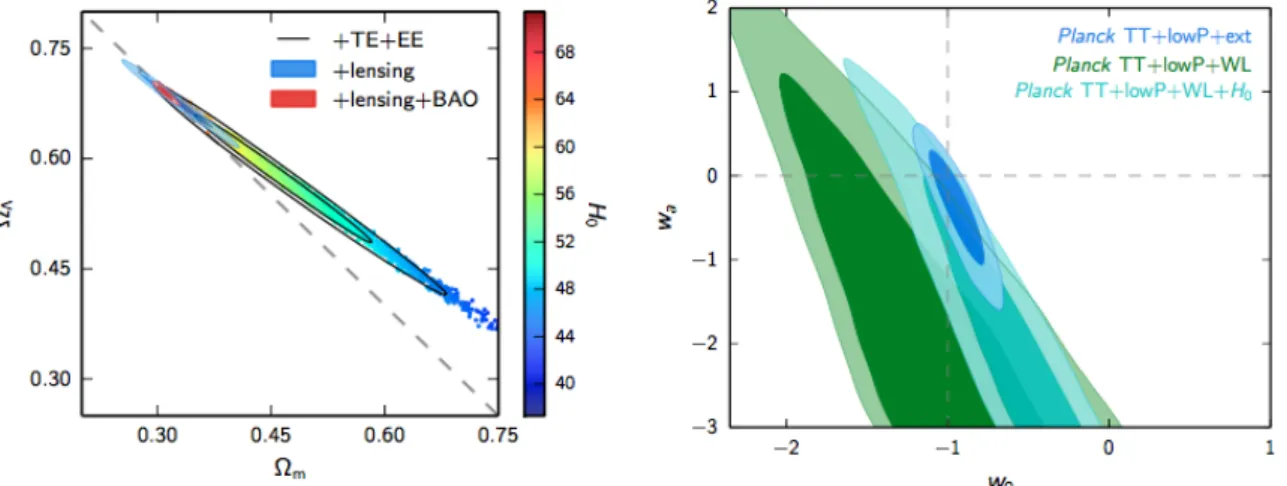
The latest constraint on the matter and dark energy content, curvature, and the dark energy equation of state parameter, from Planck and external datasets combined [15], is illustrated in the following figure.

Figure 1.1: The left plot shows the constraints on theΩm-ΩΛplane from the PlanckTT, EE, TE

and LowTEB data which is strongly constrained by the addition of lensing reconstruction and B AO data. The right plot shows the constraints on w0 and wa, for the popular CPL

parametrisation of the dark energy equation of state parameter w = w0+ (1 − a)wa, using

Planck+BAO + JLAdata. [15]

The values using the PlanckTT, EE, TEandLowTEBdata are:

Ωm= 0.3117 ± 0.007, (1.16a) ΩΛ= 0.6881 ± 0.0065, (1.16b) Ωk= 0.0002 ± 0.0021. (1.16c)

The equation of state parameter forΛ, using the Planck+lensing + externaldatasets is given by,

(1.17) _{w = −1.019}+0.075_−0.080,

which is compatible with vacuum energy, that is, a cosmological constantΛ.

1.2

Thermal History of the Universe and Recombination

It is apparent from the evolution equations for the different components (matter, radiation,Λ) of the Universe, that in a monotonically expanding universe, as we go back in time, the Universe grows denser and hotter. At sufficiently high redshifts before10−10_{s, when the Universe was}

hotter than a fewTeV, the processes that took place are beyond the energy scales that can be probed by current particle accelerators. After10−10_{shad elapsed, some of the key processes}

1.2. THERMAL HISTORY OF THE UNIVERSE AND RECOMBINATION

Different particle species were in thermal equilibrium with the background plasma. During the radiation dominated epoch, the temperature scaled as _{aT = const}. Even when matter started to dominate at redshift zeq= 3371 ± 23 [15], the high relative abundance of photons

meant the temperature of the matter-radiation plasma still scaled accordingly. As the Universe expanded and cooled, different species that were in equilibrium with the surrounding thermal bath, ’decoupled’ or ’froze out’. Each particle species has a certain reaction rateΓ with the surrounding plasma. The criterion for them to decouple from it is if the mean time between two interactions,Γ−1 _{is much greater that the cosmological time scale,H}−1_{, that isΓ}−1

À H−1. Beyond this, the reactions are not efficient enough to keep the species in equilibrium.

Figure 1.2: Table showing some of the key moments in the history of the Universe. (From DAMTP Baumann lecture notes.)

Before the background temperature dropped to the order of an eV, the high relative abundance of photons meant that there were enough high energy photons at the tail end of the Planck spectrum to ionise Hydrogen and Helium. The photons were strongly coupled to the free electrons through Compton scattering, the electrons to the nuclei by Coulomb scattering, and their mean free path was small compared to the Hubble radius. At sufficiently low energies, free electrons and protons recombined to form neutral Hydrogen atoms, an epoch known as ‘Recombination’, and the free electron density fell sharply. This allowed photons to freely stream through the transparent medium and form the Cosmic Microwave Background Radiation.

Saha equation, (1.18) µ 1 − Xe X2 e ¶ =2ζ(3) π2 η µ₂π_T me ¶32 eBHT ,

where, ζ is the Riemann function, ηis the baryon to photon ratio and is about 10−9 _at

Re-combination,me= 0.51MeVis the rest mass of electrons,BH= 13.6eVis the binding energy

of Hydrogen, and T is the temperature in energy units. The Saha equation approximately predicts the onset of Recombination but an exact solution of the electron relic density after Recombination is achieved numerically.

Figure 1.3: The figure shows the evolution of the electron fraction over time, the dashed line being the Saha approximation which correctly predicts the epoch of Recombination, and the solid line is the exact solution. The epochs of Recombination and Decoupling are defined when the electron fraction Xe falls below0.1and0.01respectively. (Figure from DAMTP Baumann

lecture notes.)

The epoch of Recombination is defined when the free electron fraction dropped to0.1. The temperature, redshift and time at Recombination is given as follows,

Trec≈ 0.3eV ≈ 3500K (1.19a) zrec≈ 1320 (1.19b) trec≈ 2.9 × 10 5 years (1.19c)

At Recombination, photons are still bound to the remaining free electrons and only decouple from them when the average time between photon-electron scattering falls belowH−1_{and the}

1.3. INFLATION

redshift and time at this epoch is given as follows,

Tdec≈ 0.27eV ≈ 3100K (1.20a) zdec≈ 1100 (1.20b) tdec≈ 3.8 × 10 5 years (1.20c)

This is the epoch at which the last scattering surface is present.

1.3

Inflation

The scenario presented above for the evolution of the Universe produces two major problems when it comes to reconciling with observational data. These two issues can be summarised as the Horizon and the Flatness Problem. Inflation provides a solution which naturally solves these issues and also acts as a mechanism for production of the initial quantum fluctuations which seeded the young Universe, which we now see in the CMB anisotropies, and later collapsed into the cosmic structures. Let us first look at the issues with the Standard Big Bang Cosmological picture.

1.3.1 Flatness and Horizon Problem

Let us combine the matter and energy density fractions in (Equation 1.14) into a single quantity

Ω = Ωm+Ωr+ΩΛ, and leaving out the curvature term. We thus have

(1.21) |Ω−1| = k

a2_H2.

As mentioned in the previous section, theR.H.Sof (Equation 1.21) is small now, and should thus have been much smaller at earlier epochs, since the Hubble radius(aH)−1_{grows with time}

in standard cosmological scenarios. If we consider a power law for the scale factora(t) = ctn

, it can be shown for the two cases of matter and radiation dominated epochs, that

(1.22) |Ω−1| ∝

(

(1 + z)−2_{, RD}

(1 + z)−1. MD

This implies that at the Planck epoch of around10−43_{swe would expect the curvature parameter}

|Ω−1|to approach10−60_{. While this is not an issue a priori, having a cosmological parameter}

so ‘fine tuned’ is not physically acceptable since only a slight fluctuation about this value would have caused the Universe to have collapsed or grown exponentially fast soon after its formation.

We had defined the particle horizon previously (Equation 1.3) as the maximum distance null rays can travel from time0to any epochtand at present is given simply by the conformal timeτ. We can reformulate the comoving distance as

(1.23) d_PH= Z a 0 d(lna) µ ₁ aH ¶ ,

and, using the same transformation as above we may write,

(1.24) d_PH∝

(

(1 + z)−1_{, RD}

(1 + z)−12_{. MD}

The comoving horizon is then monotonically increasing and at the time of recombination must have been much smaller. Regions of space that were causally disconnected at Recombination are thus not expected to share the same statistics of anisotropies. This however goes against observation, especially that of the CMB, which shows us that the entire observable last scattering surface happens to be homogeneous and shares the same statistics.

1.3.2 Inflation as a Solution to the Flatness and Horizon Problem

The importance of the Hubble radius (aH)−1 in the horizon and flatness problem can be appreciated from (Equation 1.21) and (Equation 1.23). The Hubble radius represents the distance between two points in space at a particular epoch which will be in causal contact with each other. Since the Universe has only recently started accelerating, for most part of its history, the Hubble radius has always been increasing and hence was much smaller at earlier epochs. Inflation offers to solve the flatness and horizon problem by proposing that the Hubble radius was much larger at an earlier epoch followed by a phase of decreasing Hubble radius. This naturally solves the flatness problem by pushing the value of|Ω−1|close to0. The effect of a decreasing Hubble radius is illustrated in (Figure 1.4). Regions of space which were

Figure 1.4: Comoving Hubble radius during Inflation. At the onset of inflation, distances larger than the causal horizon today were connected as the Hubble radius was large. Inflation caused the Hubble radius to decrease so that regions of space got causally disconnected. As Inflation ceased, the disconnected regions slowly started to come back into the Horizon. (Figures taken from [8].)

within the Hubble radius before Inflation were in causal connection with each other and left it during the phase of Inflation. After Inflation ceased, these regions started coming back into the horizon. Such a scenario was first proposed by Guth, Linde, Starobinsky, Albrecht and Steinhardt [17] [18] [19]. Some reviews on the topic include [8] [20].

1.3. INFLATION

A decreasing Hubble radius may be mathematically stated as

d dt µ ₁ aH ¶ < 0, =⇒ − a¨ (aH)2> 0. (1.25)

where, for the second equation we have used the Friedmann equations (Equation 1.8). For a Universe not dominated by the cosmological constant, an accelerating universe implies that the equation of state parameter be

(1.26) w < −1

3.

Another important relation can be obtained from the definition of the Hubble parameter H, giving us,

(1.27) a¨

a= H

2

(1 −²),

where we have defined²as,

(1.28) ²= − ˙ H H2= − d(lnH) dN < 1.

To satisfy the condition of acceleration²must be smaller than1. We have also defineddN

such that

(1.29) _{dN = Hdt = d(lna),}

which measure the number of e-folds N of increase of the scale factoraduring Inflation. The number of e-folds can also be taken as the duration of Inflation and to solve the problem of flatness and horizonN should typically be around60or larger. This relation also shows that the Hubble parameter changes very slowly with each e-fold.

1.3.3 Mechanism of Inflation

To achieve the conditions, described in the previous section, of a decreasing Hubble radius and a permeating fluid with an equation of state parameter_{w < −}1₃, it is customary to introduce a scalar fieldφ. The stress-energy tensor of such a field is given by

(1.30) Tφ_µν=∂µφ∂νφ− gµν

³

∂λφ∂λφ+ V (φ)

´ .

The energy density and pressure can of such a fluid is given by the00andii elements of the stress-energy tensor. This gives us

ρφ=1 2φ˙ 2 + V (φ), (1.31a) pφ₌1 2φ˙ 2 − V (φ). (1.31b)

−1₃. This implies that the potential energy term must dominate over the kinetic energy term (1.32) 1 2 ˙ φ2 < V (φ).

The equation of motion of the fieldφcan be calculated from minimising the action given by

(1.33) S = Z d4xp_−g ·₁ 2R + 1 2g µν_∂ µφ∂νφ− V (φ) ¸ ,

where the first part is the Einstein-Hilbert action and the remaining part is due to the scalar fieldφ. Minimising thisw.r.tφgives us

(1.34) _φ¨_{+ 3H ˙φ+ V,φ= 0.}

This equation resembles a simple harmonic oscillator with a friction term3H ˙φand a forcing term

V,φ. So, as the universe accelerates with increasingH, it puts up more and more resistance to

theφfield. In a flat Universe, the Friedmann equations can be cast as follows.

H2₌8πG 3 ρ φ₌8πG 3 µ₁ 2φ˙ 2 + V (φ) ¶ , (1.35a) ˙ H + H2= −4πG 3 ¡ ρφ+ 3pφ¢ = −8πG 3 ¡_˙ φ2 − V (φ)¢ . (1.35b) 1.3.4 Slow-Roll Inflation

We rewrite the conditions for inflation in terms of the quantities derived in the previous section. The parameter²can be recast, using the Friedmann equations (Equation 1.35), as

(1.36) ²=3

2¡1 + w

φ_{¢ .}

Accelerated expansion is sustained, as we have defined before, when the kinetic energy term is subdominant to the potential energy term. In the case

(1.37) φ˙2

<< V (φ),

the equation of state parameter wφ_{→ −1} and corresponds to a de Sitter solution for the evolution of the scale factor. To ensure that acceleration is sustained for a sufficiently long time to resolve the flatness and horizon problems, we require that the parameter²also vary slowly with changing e-folds. We define a new parameterηand say that it should also be small.

(1.38) η=d(ln²)

dN = ˙

²

H_².

1.3. INFLATION

to give the potential slow-roll parameters²V andηV.

²V= 1 16πG µ_V ,φ V ¶2 , (1.39a) |ηV| = 1 8πG µ_V ,φφ V ¶ . (1.39b)

In the regime of slow-roll inflation, both potential slow-roll parameters are small in order to have a sustained phase of acceleration.

(1.40) ²V, |ηV| << 1,

and the background evolution in terms of the inflation potential is given by

H2_≈1 3V (φ) ≈ Constant, (1.41a) ˙ φ≈ −V,φ 3H, (1.41b)

and the scale factor behaves like in the de Sitter case

(1.42) a(t) ∝ eH t,

implying an accelerated phase of expansion.

The potential slow-roll parameters are related to the Hubble slow-roll parameters as

²≈²V,

(1.43a)

η≈ηV−²V.

(1.43b)

Inflation comes to an end when the slow-roll conditions are violated, and is given by the conditions

²(_{φend) = 1,}

(1.44a)

²V(φend) ≈ 1.

(1.44b)

This happens as the inflation potential steepens and the inflaton, the inflation field, picks up enough kinetic energy to equal the potential energy and break the slow-roll condition.

Inflation, very elegantly, solves the issues of flatness and horizons as well as it redshifts away unwanted relics such as topological defects and monopoles which are not observed in the present Universe. However, it will do the same for any radiation or matter that might be present and will redshift it away to nothing, leaving behind the inflaton field as the primary source of the energy density. A primary concern is then how does the Universe acquire the matter and radiation density of which we are made of. The solution to this is theorised to be a process known as ’Reheating’ which occurs as inflation ends and the inflaton field oscillates at the bottom of the potentialV (_φ)(for most models). The inflaton field undergoes a damped oscillation, decays into the particles of the standard model and commences the Hot Big Bang phase of the Universe.

1.3.5 Production of Initial Perturbations and its Statistics

The formalism of Inflation developed so far only considers the evolution of the mean of the inflaton field φ. Identifying the quantum nature of the inflaton field, we expect there to be quantum fluctuations δφabout the mean. This leads to Inflation ending at different times at different places and hence imparting a density fluctuationδρ(t, x)on the matter and radiation density.

The inhomogeneities imprinted on the CMB are of the order of 1 in 105. Since gravity attracts and makes inhomogeneities grow, the fluctuations must have been smaller early on. We thus proceed with a linear perturbation of all the quantities, the energy densities and the metric, about their mean values. This section does not attempt to give a detailed treatment of the topic and is based on the text [8].

The line element for the flat FRW metric, under a linear perturbation of the metric, can be represented in the form,

(1.45) ds2= −(1 + 2Φ)dt2+ 2aBidxidt + a

2

£(1 − 2Ψ)δi j+ Ei j¤ dxidxj,

where we have made a convenient decomposition of the perturbation terms into scalar, vector and tensor quantities defined as

Bi=∂iB − Si,

(1.46a)

E_{i j= 2∂i jE −∂i}F_j−∂jF_{i+ hi j}.

(1.46b)

Φ, Ψ, E and B are scalar fields, Si and Fi are divergence-less vector fields and hi j is a

symmetric trace-less tensor field. The convenience of this decomposition lies in the fact that these fields (X represents any of the above) can be decomposed into their Fourier modes

(1.47) X_{k(t) =}

Z

dx3X (t, x)e−ik.x,

and the different Fourier modes do not interact with each other under linear conditions. Perturbing the density and pressure field about the mean background gives

δρ(t, x) =ρ(t, x) − ¯ρ(t),

(1.48a)

δp(t, x) = p(t, x) − ¯p(t).

(1.48b)

The quantities so defined are not all gauge independent, meaning that under certain coordinate transformations, these quantities will change giving rise to spurious modes. The physical nature of any perturbation can thus be understood by constructing quantities that are gauge invariant. Only the quantity hi j is gauge invariant. One of the gauge invariant quantities,

constructed out of the ones defined above, that is of interest to us is

(1.49) R₌Ψ− H

¯

ρ+ ¯pδq, Comoving curvature perturbation.

To obtain the dynamical equations of these perturbations, we plug the perturbed metric (Equation 1.45) and the stress-energy tensor into the Einstein equation and solve for them. As noted, theSV T decomposition allows the Fourier modes of the fluctuations to not mix with each other. The solution of the Einstein equation for the scalar and tensor Fourier modes is

1.3. INFLATION

given by the Mukhanov equation which has two counterparts, one for the scalar perturbation and one for the tensor perturbation.

(1.50) v00_k+ µ k2₋z 00 z ¶ v_{k= 0,}

where we have made the substitutions

vk= ( ahk, tensor zR_k, scalar (1.51a) z2₌    a2, tensor a2φ˙2 H2= 2a 2_² , scalar (1.51b)

and we have set the Planck mass MPl= (8πG)−

1

2 _{= 1and}0 _{represents a derivativew.r.tthe}

conformal timeτwhereadτ_{= dt}.

The Mukhanov equations are in general solvable numerically. In the slow roll approximation we get some intuition. As a mode with a comoving wavenumber leaves the shrinking Hubble horizon _{(k < aH)}, the amplitude of the mode freezes and is given by its value at horizon crossing.

In a statistically isotropic and homogeneous Universe where the fluctuations are Gaussian in nature, all information is contained in the 2-point correlation function. In k − space, the primordial power spectra of the scalar and tensor modes generated by Inflation are almost scale invariant. After putting back in the Planck massMPlthey are

42s(k) = 4 2 R(k) = 1 8π2 H2 MPl 1 ² ¯ ¯ ¯_k=aH , (1.52a) 42t(k) = 2 4 2 h(k) = 2 π2 H2 M_Pl ¯ ¯ ¯ k=aH , (1.52b)

The primordial power spectra are parametrised by an amplitude Aand a spectral indexn

42s(k) = As(k∗) µ _k k_∗ ¶ns(k∗)−1+12αs(k∗) ln ³ k k∗ ´ , (1.53a) 42t(k) = As(k∗) µ _k k_∗ ¶nt(k∗) , (1.53b)

where, k_∗ is an arbitrary reference or ’pivot scale’. Notice that for historical reasons the convention for defining the scalar spectral index is ns− 1. The scalar power spectrum is

parametrised using an additional parameter called the ’running’αs which quantifies the rate of

change of spectral index withln k.

The amplitude of the tensor fluctuations is often normalised relative to the scalar fluctuation amplitude. We can define a tensor to scalar ratioras

(1.54) r =4 2 t 42s = 16² ¯ ¯ ¯ k=aH ,

The energy scale of Inflation is directly linked toras (1.55) V14_∼ ³ r 0.01 ´1₄ 1016GeV.

In the slow-roll approximation, the scalar and tensor spectra, their spectral indices and the tensor to scalar ratio are given by

42s≈ 1 24π2 V M4 Pl 1 ²V , (1.56a) 42t≈ 2 3π2 V M4 Pl 1 , (1.56b) ns− 1 = 2ηV− 6²V, (1.56c) nt= −2²V, (1.56d) r = 16²V, (1.56e)

all these quantities being calculated at the horizon crossing k = aH.

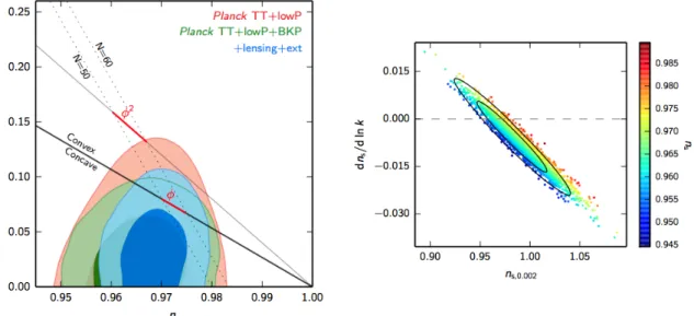
Figure 1.5: Left: The joint constraint on the tensor to scalar ratio rand the scalar spectral indexn_s, from a joint Planck and BICEP analysis, assuming a baseCDMmodel withras an additional parameter. Right: This figure shows the constraints on the running of the spectral index. This is done by adding running as an additional parameter and takingr = 0over a base

ΛCDMmodel. (Figures taken from [15].)

At present, the best constraints on some of the Inflationary parameters have been obtained by the Planck satellite with the addition of external datasets such as the BICEP/Keck [15] [21]. The scalar spectral index provides a slight red tilt to the scalar power spectrum. A definitive measurement of the tensor to scalar ratio has not been possible yet and only upper limits are

1.4. IMPRINTS ON THE CMB : ANISOTROPIES provided onr ns= 0.968 ± 0.006, (1.57a) r < 0.09, 95%CL, (1.57b) dns d ln k= −0.0065 ± 0.0076. (1.57c)

1.4

Imprints on the CMB : Anisotropies

As the inflationary phase comes to an end, it leaves behind an almost scale independent density fluctuation on the matter and radiation in the Universe, as well as an expected background of almost scale independent gravitational waves. The density fluctuations at different length scales remain frozen as long as their corresponding comoving modeskare outside the horizon

(k < aH). After the end of Inflation, the Hubble radius starts to increase, progressively more and more modes enter the horizon and are able to evolve. Starting with the smallest scales first, the gravitational pull of baryonic and dark matter and pressure from the radiation density undergoes a balancing act. Gravity causes over-dense regions to collapse and radiation pressure opposes it. Moreover, the baryonic matter is strongly coupled to the radiation field through Compton scattering. This interplay between the different components, set up on an expanding FRW frame, gives rise to standing waves in the hot plasma that evolve over time. At the epoch of ‘Decoupling’, the radiation is free to stream through the newly transparent Universe and forms the Cosmic Microwave Background radiation. Having been in thermal equilibrium with the baryonic matter, the CMB radiation carries an imprint of the density fluctuations at the last scattering surface and hence acts as a direct probe of the physical processes that led to the production of these fluctuations. Discussions on which this section is based are [9] [22].

1.4.1 Primary Temperature Anisotropies

The primary CMB anisotropies are those that are intrinsic to the last scattering surface that were produced by physical processes leading up to and during last scattering. The primary temperature anisotropies predominantly evolved from the primordial scalar fluctuations R and can be explained by three physical processes:

• The intrinsic temperature variation on the last scattering surface.

• The Sachs-Wolfe effect [23], which describes the gravitational red and blue-shifting of photons as they leave the gravitational potential well of the matter over and under-densities at the last scattering surface.

• Doppler shift due to the bulk motion of the baryonic matter at the last scattering surface. Schematically, the anisotropies may be described by a scalar field Θtot, equal to the

temperature anisotropies of the CMB radiation at the last scattering surface.

(1.58) Θtot=4T T = [(Ψ+Θ)− ˆr· v] ¯ ¯ ¯_τ=τ dec ,

where,Θis due to the baryonic density fluctuation,Ψis the Newtonian gravitational potential andvis the velocity field of the bulk baryonic matter. These quantities have all been calculated

at the last scattering surfaceτ=τdec. It is most convenient to work with the Fourier modes of

these quantities as in the linear theory, each of the_{k − modes}evolve independently.

To determine the evolution of the modes that have re-entered the horizon we have to solve the complete set of equations of the perturbation theory. For the non-relativistic species these are the continuity equation, the Euler equation and the Poisson equation, and for the relativistic species it is the Boltzmann equation.

After the end of Inflation and before Decoupling, there were two distinct regimes, a radiation dominated one and a matter dominated one where the scale factoraevolved differently as given in (Table 1.1). We assume that the matter content is mostly composed of Cold Dark Matter(CDM) whose perturbation evolution is given by

(1.59) δ¨CDM+ 2 ˙ a a ˙ δCDM− 4πG ¯ρδCDM= 0,

whereδCDM is the CDM density perturbation andρ¯ is the mean density of the CDM. Since the

CDM does not interact electromagnetically, the only forcing term is gravity. During the radiation dominated epoch,ρ¯ is small andδdoes not grow. In the matter dominated epoch, the solutions areδCDM∝ t

2 3 _andδ

CDM∝ t−1. The growing mode solution implies the gravitational potentialΨ

is time independent.

The photon and ionised baryonic fluid are tightly coupled together by means of Compton scattering. Due to the strong coupling, its velocity fieldv_B, temperatureT and the photon phase-space distribution function f_γare completely determined by the baryonic density fluctuationδB.

Θis related to the baryonic density fluctuation by

(1.60) Θ(t) =1

3δB(t).

Using units in whichc = 1, the dynamics of the photon-baryon fluid for each individualk-mode is given by (1.61) d dτ£(1 + R) ˙Θ¤+ k2 3Θ = − k2 3 (1 + R)Ψ, where,R = 3ρB

4ργ is the ratio of the baryon and photon energy density. This is the differential

equation for a simple harmonic oscillator with a driving term on the right that is purely grav-itational. It leads to a plane-wave solution for each Fourier mode propagating through the photon-baryon medium with a particular sound speed. Starting off with a flat spectrum at time

τ= 0, the oscillations evolve into a harmonic series of acoustic peaks corresponding to modes that were at their extremum atτdec. The Doppler shift due to the bulk motionv of the plasma

has a plane wave solution too that is subdominant in amplitude and is out of phase by90° in time and space with the other two effects.

The phenomenon of “Silk damping” is related to the thickness of the transition between the strongly coupled phase to the free-streaming of photons during Decoupling. Modes that were on scales smaller than the thickness of the last scattering surface get damped.

The temperature anisotropies measured on the sky are not computed in the Fourier space but in the real space as a function of the positionnˆ on the sphere. The temperature anisotropy

1.4. IMPRINTS ON THE CMB : ANISOTROPIES

field can be decomposed in the basis of the spherical harmonics

T( ˆ_{n) − T}0 T0 = 4T( ˆn) T0 = X lm almYlm( ˆn), alm= Z dΩYlm( ˆn)∗µ 4T( ˆn) T0 ¶ . (1.62)

Ifalmis a Gaussian random variable, as is predicted from Inflation, the information content is

contained in the power spectrum

(1.63) CT T_{l =} 1 2l + 1 X m ­a∗ lmalm ®

This is what is measured when we observe the CMB sky hence we want to translate the fluctuations we see in thek − spaceto the anisotropies in thel − space. To obtain the primary anisotropies on the CMB, in the harmonic space, we project the fluctuations ink − spaceat the last scattering surface to_{l − space}. The projection operator is obtained by the Bessel function

jl(kD∗), where D∗=τ0−τ∗ is the distance from us to the last scattering surface, a (. . . )∗

meaning it’s value at the last scattering surface, and the anisotropies are given by (1.64) al(k) =Θtot(τ∗) jl(kD∗)

This gives us the temperature anisotropy power spectrum in terms of the primordial inflationary power spectrum as (1.65) CT T_{l = 4}πX lm Ylm( ˆn) · (−i)l Z _d3_k (2π)3al(k)Y ∗ lm( ˆk) ¸

The Bessel function jl(kD∗)is strongly peaked atkD∗≈ l and hence most of the power in the

modekis mapped to its corresponding mode inl.

In an expanding FRW frame, the potential well of the intervening matter over-densities decay over time and this becomes more pronounced during an accelerating dark energy dominated phase, as it is at the present epoch. The CMB photons that traverse these potential wells see a shallower potential well coming out than when falling into it leading to an energy boost. This is known as the “Sachs-Wolfe effect”. The change in the temperature is quantified by integrating this effect along the line of sight from the last scattering surface to us and is given by (1.66) µ 4T T ¶ ISW = Z £_˙ Ψ(τ) − ˙Φ(τ)¤ dτ,

where,ΦandΨhave their usual meaning.

Close to the Decoupling epoch the CMB also undergoes an early ISW effect. This is due to the fact that the radiation energy density is non-negligible after Decoupling and radiation pressure damps any fluctuation of the potential that enter the horizon, well into the matter dominated epoch. The effect is on the large scales corresponding to modes which oscillate on time scales comparable to the potential decay time.

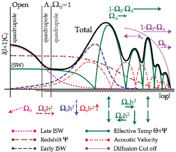
Figure 1.6: The figure shows how the different processes contribute to the temperature power spectrum. The acoustic peaks (green) are given by the perturbations in the matter density fluctuations and the gravitational potential, also showing the Sachs-Wolfe plateau at low multipoles. The bulk velocity (dashed red) produces fluctuations which are subdominant and out of phase by90° to the previous process. The Late ISW (dashed pink) shows a significant contribution at the low multipoles and the diffusion damping (Silk damping) envelope (dotted pink) shows the suppression of power at high multipoles. (Figure taken from [24].)

1.5

Polarisation of the CMB

The CMB radiation, as shown above, encodes the information of the matter density fluctuation and the bulk velocity at the last scattering surface in the temperature power spectrum and thus acts as a direct probe of the physical processes that take place before Decoupling. Compton scattering of photons with the free electrons partially polarises the CMB and the polarisation signal contains additional information. Most importantly, the production of gravitational waves from the Inflationary epoch are expected to produce a distinct signature on the CMB polarisation and is therefore the most powerful probe to test the parameters of Inflation and differentiate between different models that produced the primordial fluctuations.

1.5. POLARISATION OF THE CMB

1.5.1 Representation of Polarisation

In the previous section we have described how the temperature anisotropy field, given by a scalar quantity as a function of position on the sky, can be decomposed in a basis of spherical harmonics. The complete radiation field, including intensity and polarisation, can be represented in the basis of the Stokes parameters(I, Q,U, V )[25]. The StokesV parameter is not known to be generated by any processes relevant to the CMB and hence will be dropped. Unlike the scalar I, the Stokes parameters Q andU are dependent on the local reference frame at the point of measurement, and hence, we wish to perform a linear transformation to quantities which are scalar and invariant upon rotation of the local coordinate frame. Upon a rotation by an angleψ, theQandU Stokes parameters transform as,

(1.67) (Q ± iU)0= e∓2iψ(Q ± iU)

The quantity(Q ± iU)is thus a spin-2quantity and must be decomposed in a basis of spin weighted spherical harmonics. We can thus decompose all three Stokes parameters in the following manner, (1.68) (Q ± iU)( ˆn) =X l X m a_{±2,lm ±2}Y_lm( ˆn)

where,Ylm and±2Ylmare the spherical harmonic functions and the spin-weighted harmonic

functions respectively. The harmonic coefficients can be easily obtained from (Equation 1.67) by employing the orthogonality property of the harmonic functions,

a2,lm= · (l + 2) (l − 2) ¸−12Z dΩY_lm∗ ( ˆ_n)6∂2(Q + iU)( ˆn) (1.69a) a_−2,lm= · (l + 2) (l − 2) ¸−12Z dΩY_lm∗ ( ˆ_{n) 6}∂2(Q − iU)( ˆn) (1.69b)

where,6∂and6∂are raising and lowering operators of the harmonic functions as given in [26]. We now define a linear combination of these harmonic coefficients as follows,

aE,lm= − 1 2¡a2,lm+ a−2,lm ¢ (1.70a) a_{B,lm= −}i 2¡a2,lm− a−2,lm ¢ (1.70b)

These quantities behave differently under a parity transformation.Eremains unchanged andB

reverses sign.

If the fluctuations on the CMB sky are Gaussian, the statistics of these fluctuations can be characterised completely by the two point correlation functions and hence by their har-monic transforms, the power-spectra. Four non-vanishing spectra can be constructed from the

quantities defined above CEE₌ 1 2l + 1 X m D a∗_E,lma_E,lmE, (1.71a) CBB₌ 1 2l + 1 X m D a∗_B,lma_B,lmE, (1.71b) CT E= 1 2l + 1 X m D a∗_T,lmaE,lm E , (1.71c)

with the fourth spectrumCT T defined earlier. When the polarisation amplitude is represented on the sky using ’rods’ of a given magnitudeP at a certain orientationα, in the local coordinate system, they are defined as

P = q Q2 +U2 , (1.72a) α=1 2tan −1 µ_Q U ¶ , (1.72b)

1.5.2 Thomson Scattering of Photons

The Thomson scattering is the low energy limit of Compton scattering and is the principal scattering mechanism at the last scattering surface. Qualitatively, the process of Thomson scattering re-emits polarised radiation from incident unpolarised radiation that is direction dependent. An anisotropic radiation field, such as was present at the last scattering surface, would thus create a net polarisation in the direction of the observer. To quantify the polarisation of the radiation we consider the Stokes(I, Q,U)parameters. In the rest frame of the electron, the Stokes parameters of the scattered radiation due to an anisotropic field of incident unpolarised radiation are given by [27]

I_sca= 3σT 16πσ Z dΩ(1+cos2_θ)I_inc(_θ,_φ), (1.73a) Q_sca= 3σT 16πσ Z

dΩsin2_θcos(2_φ)I_inc(_θ,_φ),

(1.73b)

U_{sca= −} 3σT 16πσ

Z

dΩsin2_θsin(2_φ)I_inc(_θ,_φ),

(1.73c)

where,σTis the Thomson scattering cross-section. Decomposing the incident radiation into its

spherical harmonic components, the scattered Stokes(I, Q,U)can be restated as

I_sca=3σT 16π ·₈ 3 p πa₀₀₊4 3 r_π 5a20 ¸ , (1.74a) Qsca= 3σT 4π s 2π 15Re(a22), (1.74b) Usca= − 3σT 4π s 2π 15Im(a22), (1.74c)

wherea22is the spin-2quadrupole coefficient in the harmonic decomposition of the incident

1.6. LATE TIME COSMOLOGY WITH THE CMB

radiation if the electron, in its rest frame, sees a quadrupole anisotropy in the incident radiation. It’s also to be noted that only the _{m = ±2}quadrupole moment, which coincide with anisotropies in the plane orthogonal to the direction of the observer, produce a net polarisation. Along the line of sight of the observer, the net effect will be determined by how each type of quadrupole anisotropy_{(m = 0,±1,±2)}project ontom = 2. A review of CMB polarisation, relevant for this and the next subsection is given in [28].

1.5.3 Sources of Quadrupole

The CMB photons that travel to us from the last scattering surface are polarised by quadrupolar anisotropies in the radiation field the electron sees in its rest frame. The different ways such a quadrupole can be generated are listed below.

• Scalar : The scalar modes are related to the perturbations in the density field that were shown previously. As the electron-photon fluid is accelerated towards an over-density, it sees the radiation field in the radial direction being redshifted away from it whereas in the perpendicular direction it sees a blue-shifting. This leads to the electron, in its rest frame, seeing a quadrupole anisotropy. Considering the line of sight from the electron at the last scattering surface to us, the net polarisation pattern is radial to the over-density. The converse happens when the electron comes out of an under-dense region and the net polarisation is oriented tangentially to the under-density.

• Vector : The vector perturbations give the velocity field a divergence-free but non-zero curl component. Vector modes are expected to decay very fast, so at the time of last scattering they are not expected to have any contribution.

• Tensor : The tensor modes are related to the metric perturbations during Inflation lead-ing to the production of gravitational waves. As gravitational waves pass through the plasma they cause a compression and rarefaction in orthogonal directions leading to the formation of quadrupolar anisotropies in the rest frame of the electron. Depending upon the polarisation state of the gravitational wave, it produces a curl-like feature in the polarisation vector field on the sky as well as the type of pattern describes for scalar modes.

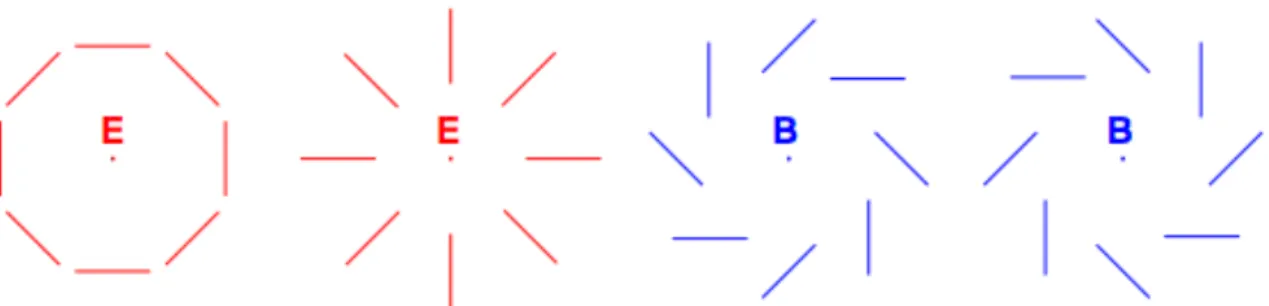
The polarisation patterns described above are illustrated in (Figure 1.7). The two classes of patterns are known as the E and B modes and are produced by different sources of anisotropies. These are directly related to the anisotropiesaE,lm andaB,lm and hence provide a convenient

method of probing the source of the perturbations. Tensor perturbations produce both E and B mode polarisation as well as contribute sub dominantly to the temperature anisotropies. How-ever, scalar perturbations can only produce E mode polarisation and temperature anisotropies. Ab initio, the scalar and tensor perturbations were produced by inflation, thus observation of primordial B-modes are currently the best method of probing the physics and energy scale of Inflation.

1.6

Late time Cosmology with the CMB

The CMB photons that have been freed from the strong coupling with the ionised baryonic matter at the last scattering surface have been travelling to us for the rest of the history of the

Figure 1.7: The polarisation patterns created by different sources of quadrupolar anisotropy seen by the electrons at the last scattering surface. The E modes are a curl-free pattern, generated by both scalar and tensor perturbations while the B modes are a divergence-free pattern, flipping under a parity transformation, produced by tensor perturbations that are due to primordial gravitational waves. (Figure taken from [29].)

Universe. The CMB therefore not only acts as a probe of the physical processes that happened prior to last scattering but also acts as a backlight to all the intervening matter between us and its source. The CMB photons keep on gravitationally interacting with the intervening matter field along the line of sight. These interactions cause the trajectory of these photons to be altered and hence distort the primary CMB sky. With the birth of the first stars, the UV radiation emitted by them caused the neutral Hydrogen to re-ionise and hence scatter the CMB photons. The CMB photons are also inverse Compton scattered by high energy electrons in galaxy clusters, which alters the shape of its spectra. The influence of all these effects is encoded on the CMB temperature and polarisation power spectra as secondary anisotropies as well as on the matter power spectrum.

1.6.1 Weak gravitational lensing

The CMB photons on their way from the last scattering surface to us encounter the intervening matter distribution. The interaction of the photons with the gravitational potential of the clusters, which are primarily made up of dark matter, lead to deviations in their trajectories. This causes what is known as weak gravitational lensing, small deflections in the photon trajectories that are small enough to be treated accurately up to first order approximations. The lensing of the primary CMB anisotropies conserves its brightness but remaps the anisotropies across the sky. The angular deflection fieldαof a CMB photon from the last scattering surface to us, after multiple deflections by gravitational potentialsΨ, under the Born approximation [30] is given by

(1.75) α= −2

Z χ_∗

0

d_χ fK(χ∗−χ)

f_K(_χ∗) f_K(_χ)∇nˆΨ(χn;ˆ τ0−χ)

where, in a flat FRW universe, fK(χ) =χ= r is the comoving distance, ∇nˆ is the gradient

operator along the line of sight, andτ0−χgives the time at which the photon was at position χnˆ and the integration is from the observer at the origin to the last scattering surfaceχ∗. The

angular deflection is also known as the deflection field and is a function of the positionnˆ on the sky.

Using the formula for the deflection angle (Equation 1.75) we may define a lensing potential