Université de Montréal
On Two Sequential Problems: The Load Planning and
Sequencing Problem and the Non-normal Recurrent
Neural Network
par
Kyle Goyette
Département d’informatique et de recherche opérationelle Faculté des arts et des sciences
Mémoire présenté en vue de l’obtention du grade de Maître ès sciences (M.Sc.)
en informatique
July 23, 2020
c
Université de Montréal
Faculté des études supérieures et postdoctoralesCe mémoire intitulé
On Two Sequential Problems: The Load Planning and Sequencing
Problem and the Non-normal Recurrent Neural Network
présenté par
Kyle Goyette
a été évalué par un jury composé des personnes suivantes :
Fabian Bastin (président-rapporteur) Emma Frejinger (directeur de recherche) Pierre L’Écuyer (membre du jury)
Abstract
The work in this thesis is separated into two parts. The first part deals with the load planning and sequencing problem for double-stack intermodal railcars, an operational problem found at many rail container terminals. In this problem, containers must be assigned to a platform on which the container will be loaded, and the loading order must be determined. These decisions are made with the objective of minimizing the costs associated with handling the containers, as well as minimizing the cost of containers left behind. The deterministic version of the problem can be cast as a shortest path problem on an ordered graph. This problem is challenging to solve because of the large size of the graph. We propose a two-stage heuristic based on the Iterative Deepening A* algorithm to compute solutions to the load planning and sequencing problem within a five-minute time budget. Next, we also illustrate how a Deep Q-learning algorithm can be used to heuristically solve the same problem.
The second part of this thesis considers sequential models in deep learning. A recent strategy to circumvent the exploding and vanishing gradient problem in recurrent neural networks (RNNs) is to enforce recurrent weight matrices to be orthogonal or unitary. While this ensures stable dynamics during training, it comes at the cost of reduced expressivity due to the limited variety of orthogonal transformations. We propose a parameterization of RNNs, based on the Schur decomposition, that mitigates the exploding and vanishing gradient problem, while allowing for non-orthogonal recurrent weight matrices in the model.
Key words: Intermodal rail terminal, containers, rail, train, double-stack, load planning and sequencing, dynamic programming, deep reinforcement learning, sequential modelling, recurrent neural networks, exploding and vanishing gradient problem
Sommaire
Le travail de cette thèse est divisé en deux parties. La première partie traite du problème de planification et de séquencement des chargements de conteneurs sur des wagons, un prob-lème opérationnel rencontré dans de nombreux terminaux ferroviaires intermodaux. Dans ce problème, les conteneurs doivent être affectés à une plate-forme sur laquelle un ou deux conteneurs seront chargés et l’ordre de chargement doit être déterminé. Ces décisions sont prises dans le but de minimiser les coûts associés à la manutention des conteneurs, ainsi que de minimiser le coût des conteneurs non chargés. La version déterministe du problème peut être formulé comme un problème de plus court chemin sur un graphe ordonné. Ce problème est difficile à résoudre en raison de la grande taille du graphe. Nous proposons une heuristique en deux étapes basée sur l’algorithme Iterative Deepening A* pour calculer des solutions au problème de planification et de séquencement de la charge dans un budget de cinq minutes. Ensuite, nous illustrons également comment un algorithme d’apprentissage Deep Q peut être utilisé pour résoudre heuristiquement le même problème.
La deuxième partie de cette thèse examine les modèles séquentiels en apprentissage pro-fond. Une stratégie récente pour contourner le problème de gradient qui explose et disparaît dans les réseaux de neurones récurrents (RNN) consiste à imposer des matrices de poids récurrentes orthogonales ou unitaires. Bien que cela assure une dynamique stable pendant l’entraînement, cela se fait au prix d’une expressivité réduite en raison de la variété limitée des transformations orthogonales. Nous proposons une paramétrisation des RNN, basée sur la décomposition de Schur, qui atténue les problèmes de gradient, tout en permettant des matrices de poids récurrentes non orthogonales dans le modèle.
Mots-clés: Transport ferroviaire intermodal, conteneurs, planification et séquencement des chargements, programmation dynamique, apprentissage par renforcement profond, modéli-sation séquentielle, réseaux de neurones récurrents
Contents
Abstract . . . . 5 Sommaire . . . . 6 List of Tables . . . . 12 List of Figures . . . . 15 List of Abbreviations . . . . 16 Acknowledgements . . . . 18Part 1. The Load Planning and Sequencing Problem . . . . 19
Chapter 1. Introduction: The Load Planning and Sequencing Problem . . . 20
1.1. Rail Transportation of Containerized Cargo . . . 21
1.1.1. Containers . . . 21
1.1.2. Railcars, Platforms and Slots . . . 21
1.1.3. Intermodal Container Terminals. . . 22
1.1.4. Handling Equipment . . . 22
1.1.5. The Load Planning and Sequencing Problem . . . 23
1.2. Methodologies . . . 24
1.2.1. Introduction to Dynamic Programming . . . 24
1.2.2. Artificial Neural Networks and Deep Reinforcement Learning . . . 25
Chapter 2. . . . . 29
First Article. Heuristics for the Load Planning and Sequencing Problem . . . 29
Author Contributions . . . 29
2.1. Introduction . . . 30
2.2. The Load Planning and Sequencing Problem for Double-Stack Intermodal Trains . . . 31
2.2.1. Retrieving Containers from the Storage Area . . . 32
2.2.2. Assignment of Containers to Railcars . . . 35
2.3. Related Literature . . . 36
2.4. Mathematical Formulation . . . 38
2.4.1. States and Actions of the LPSP . . . 38
2.4.2. Cost . . . 39
2.5. Heuristics . . . 41
2.5.1. Calculation of a Lower Bound . . . 41
2.5.2. A Two-stage Heuristic . . . 42
2.5.2.1. Phase 1: Beam Search . . . 42
2.5.2.2. Phase 2: IDA* DFS State Space Search . . . 43
2.5.3. Leveraging Problem Structure to Reduce the Search Space . . . 46
2.6. Numerical Study . . . 47
2.6.1. Problem Instances . . . 47
2.6.2. Model Parameters . . . 47
2.6.3. Baselines . . . 48
2.6.4. Results . . . 49
2.6.4.1. Small Costs: 2-way Distance Function . . . 50
2.6.4.2. Small Costs: 1-way Distance Function . . . 53
2.6.4.3. Small Costs: 0-way Distance Function . . . 57
2.6.4.4. Large Costs: 2-way Distance Function . . . 58
2.6.4.5. Large Costs: 1-way Distance Function . . . 60
2.6.5. Comparison of Results for Different Distance Functions . . . 63
2.6.6. Discussion . . . 64
2.7. Conclusion . . . 67
Acknowledgements . . . 67
2.8. Appendix . . . 68
2.8.1. Proof of Propostion 1 . . . 68
2.8.1.1. Notation and Introduction . . . 68
2.8.1.2. Proof for Fixed q . . . 68
2.8.1.3. Final Step of the Proof . . . 70
Second Article. Load Planning and Sequencing with Deep Q-Networks . . . . 71
Author Contributions . . . 71
3.1. Introduction . . . 72
3.2. Literature Review . . . 73
3.3. Methodology . . . 74
3.3.1. The Load Planning and Sequencing Problem . . . 75
3.3.2. State Representation . . . 75
3.3.2.1. Storage Area. . . 76
3.3.2.2. Double-touched Containers . . . 77
3.3.2.3. Platforms . . . 77
3.3.3. Action Representation . . . 80
3.3.4. Neural Network Architecture . . . 80
3.3.5. Training . . . 82
3.3.6. Beam Search with DQN. . . 82
3.4. Experiments . . . 83
3.4.1. Instance Generation and Environment Cost Values . . . 83
3.4.2. Hyperparameters . . . 84
3.4.3. Numerical Results . . . 85
3.4.3.1. Small Distance Cost Results . . . 85
3.4.3.2. Large Cost Value Results . . . 90
3.5. Discussion . . . 95
3.6. Conclusion . . . 97
Acknowledgements . . . 97
Part 2. Learning Long-term Dependencies While Increasing Expressivity in Sequential Models . . . . 98
Chapter 4. Introduction: Recurrent Neural Networks and the Exploding and Vanishing Gradient Problem . . . . 99
4.1. Recurrent Neural Networks . . . 99
4.2. The Exploding and Vanishing Gradient Problem . . . 100
Chapter 5. . . . 102
Third Article. Non-normal Recurrent Neural Network (nnRNN): learning long time dependencies while improving expressivity with transient dynamics . . . 102
Author Contributions . . . 103
5.1. Introduction . . . 103
5.2. Background . . . 104
5.2.1. Unitary RNNs and constrained optimization . . . 104
5.2.2. Non-normal connectivity . . . 105
5.3. Non-normal matrices are more expressive and propagate information more robustly than orthogonal matrices . . . 106
5.3.1. Non-normality drives expressive transients . . . 107
5.3.2. Non-normality allows for efficient information propagation. . . 107
5.3.3. Non-normal matrix spectra and gradient propagation. . . 109
5.4. Implementing a non-normal RNN . . . 110
5.5. Numerical experiments . . . 111
5.5.1. Copy task & permuted sequential MNIST . . . 111
5.5.2. Penn Treebank (PTB) character-level prediction . . . 112
5.5.3. Analysis of learned connectivity structure . . . 113
5.6. Discussion . . . 114
Acknowledgements . . . 115
5.7. Appendix . . . 117
5.7.1. Task setup and training details . . . 117
5.7.1.1. Copy task . . . 117
5.7.1.2. Sequential MNIST classification task . . . 118
5.7.1.3. Penn Treebank character prediction task . . . 118
5.7.1.4. Hyperparameter search . . . 119
5.7.2. Fisher memory curves for strictly lower triangular matrices . . . 120
5.7.3. Proof of proposition 4 . . . 122
5.7.4. Numerical instabilities of the Schur decomposition . . . 122
5.7.5. Learned connectivity structure on psMNIST . . . 122
Part 3. Concluding Remarks . . . 125 Chapter 6. Conclusion . . . 126 6.1. The Load Planning and Sequencing Problem . . . 126 6.2. Learning Long-term Dependencies While Increasing Expressivity in Sequential
Models . . . 127 Bibliography . . . 129
List of Tables
2.1 Example of an AAR Guide loading pattern . . . 35
2.2 Handling cost definition values for different distance functions . . . 41
2.3 Characteristics of problem instances . . . 48
2.4 Cost parameters for each distance function in all experiments . . . 48
2.5 Cost parameters and environment variables which remain constant across distance functions . . . 48
2.6 Heuristics abbreviations and descriptions . . . 49
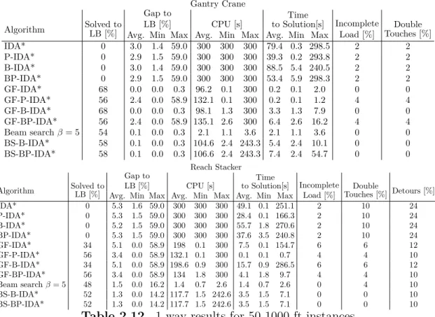
2.7 2-way results for 50 200-ft instances . . . 51
2.8 2-way results for 50 1000-ft instances . . . 52
2.9 2-way results for 50 1500-ft instances . . . 52
2.10 2-way results for 50 2000-ft instances . . . 53
2.11 1-way results for 50 667-ft instances . . . 54
2.12 1-way results for 50 1000-ft instances . . . 55
2.13 1-way results for 50 1500-ft instances . . . 56
2.14 1-way distance functions for 50 2000-ft instances . . . 56
2.15 0-way results for 50 667-ft instances . . . 57
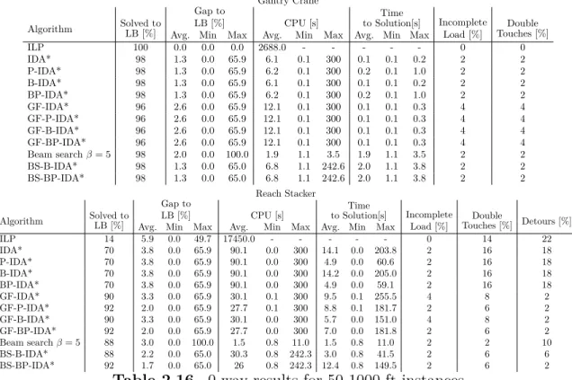
2.16 0-way results for 50 1000-ft instances . . . 58
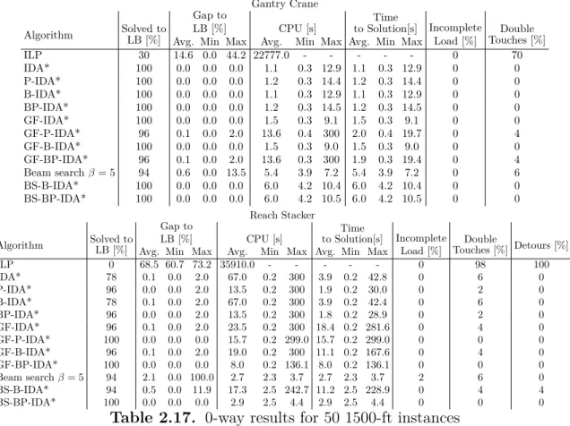
2.17 0-way results for 50 1500-ft instances . . . 59
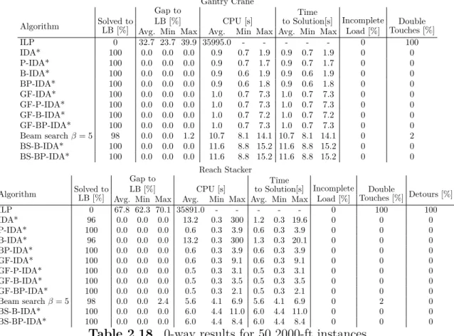
2.18 0-way results for 50 2000-ft instances . . . 60
2.19 2-way results for 50 1000-ft instances using large cost values . . . 61
2.20 2-way results for 50 1500-ft instances using large cost values . . . 61
2.21 2-way results for 50 2000-ft instances using large cost values . . . 62
2.22 1-way results for 50 1000-ft instances using large cost values . . . 62
2.23 1-way results for 50 1500-ft instances using large cost values . . . 63
2.25 Gap to LB of distance travelled using solutions meeting LB from each distance
function on the 2-way distance function for small cost values . . . 65
2.26 Gap to LB using solutions meeting LB from each distance function on the 2-way distance function for small cost values. . . 65
2.27 Gap to LB of distance travelled using solutions meeting LB from each distance function on the 2-way distance function for small cost values . . . 65
2.28 Gap to LB using solutions meeting LB from each distance function on the 2-way distance function for large cost values . . . 66
3.1 Environment costs . . . 84
3.2 Training hyperparameters . . . 84
3.3 Medium size training problems . . . 86
3.4 Medium size validation problems . . . 87
3.5 Medium size test problems . . . 87
3.6 Large size training problems . . . 88
3.7 Large size validation problems . . . 88
3.8 Large size test problems . . . 89
3.9 Largest size training problems . . . 89
3.10 Largest size validation problems . . . 90
3.11 Largest size test problems . . . 90
3.12 Medium size training problems using large cost values . . . 92
3.13 Medium size validation problems using large cost values . . . 92
3.14 Medium size test problems using large cost values . . . 93
3.15 Large size training problems using large cost values . . . 93
3.16 Large size validation problems using large cost values . . . 94
3.17 Large size test problems using large cost values . . . 94
3.18 Largest size training problems using large cost values . . . 95
3.19 Largest size validation problems using large cost values. . . 95
3.20 Largest size test problems using large cost values . . . 96
5.1 PTB test performance bit per character (BPC) for sequence lengths TP T B = 150, 300 . . . 112
5.2 Hyperparameters for the copy task . . . 117 5.3 Hyperparameters for the permuted sequential MNIST task . . . 119 5.4 PTB test performance: Test Accuracy . . . 119 5.5 Hyperparameters for the Penn Treebank task (at 150 and 300 time step truncation
for gradient backpropagation) . . . 120 5.6 Fisher memory curve performance: Shown is the sum of the FMC for the models
considered in section 5.3. . . 121 5.7 PTB test performance: bits per character (BPC) . . . 124
List of Figures
1.1 A double-stack train composed of several railcars, loaded with containers . . . 22 1.2 A gantry crane loading a container onto a railcar . . . 23 1.3 A reach stacker holding a container . . . 23 2.1 An overhead view of the railroad container terminal considered (taken from [67]) 32 2.2 Schematic designs of gantry cranes and reach stackers . . . 33 2.3 Summary of forbidden loading operations for a reach stacker (adapted from [67]) 34 2.4 IDA* update algorithm . . . 44 3.1 Overview of architecture of neural network model . . . 81 3.2 Performance of model on training set when training on small cost values . . . 86 3.3 Performance of model on training set when training on uneven small cost values . 91 5.1 Benefits of non-normal dynamics . . . 106 5.2 Cross entropy of each model on copy task (left) and permuted sMNIST (right) . . 111 5.3 Learned Θs show decomposition into Λ and T . . . 114 5.4 Model performance on copy task (left) and permuted sequential MNIST (right)
with same number of trainable parameters . . . 118 5.5 Learned Θ on psMNIST task. Inset: angles θi distribution of block diagonal
rotations. (cf. Eq.5.4). . . 123 5.6 Gradient propagation for each model across time steps . . . 124
List of Abbreviations
AAR Association of American Railroad ADP approximate dynamic programming ANN artificial neural network
BFS breadth-first search
BPC bits per character
BPTT backpropagation through time CNN convolutional neural network
DFS depth-first search
DP dynamic programming
DQN deep Q-network
DRL deep reinforcement learning
EURNN efficient unitary recurrent neural network EVGP exploding and vanishing gradient problem expRNN exponential recurrent neural network
FMC Fisher memory curve
GRU gated recurrent unit
LB lower bound
LDFS learning depth-first search
LPP load planning problem
LPSP load planning and sequencing problem
LSP load sequencing problem
LR learning rate
LSTM long short-term memory
NLP natural language processing
nnRNN non-normal recurrent neural network
PTB Penn Treebank
ReLU rectified linear unit
RL reinforcement learning
RNN recurrent neural network
SDMP sequential decision-making process SGD stochastic gradient descent
SVD singular value decomposition SSPP ship stowage planning problem
Acknowledgements
I’d like to express my thanks to Dr. Emma Frejinger for her excellent guidance and leadership throughout the project. I’d also like to thank Dr. Guillaume Lajoie for his leadership on the nnRNN project. We are grateful to Eric Larsen for his valuable comments that helped improve this manuscript.
Part 1
Chapter 1
Introduction: The Load Planning and Sequencing
Problem
Rail transportation of containerized cargo is a sustainable mode, being both environmentally friendly and cost effective, for long-distance ground transportation of containers inland for the North American market. The number of containers shipped via rail has been growing consistently since 2016, to more than 30 million containers in 2018. Double-stack railcars, introduced in 1984 in North America, allow for twice as many containers to be shipped, making rail an efficient mode of long-distance ground container transportation. Crucial to the continued growth of rail transportation is the efficient operation of rail terminals, wherein containers are loaded and offloaded from railcars.
The load planning and sequencing problem (LPSP) is the focal point of this work. It jointly considers the assignment of containers to platforms and the sequence of operations to place containers on platforms such that the value of containers loaded onto the plat-forms is maximized, and the cost of handling containers is minimized. The selection of containers must meet constraints defined by the railcar specifications and weight distribu-tion requirements defined by guides from the Associadistribu-tion of American Railroads (AAR). This combinatorial optimization problem was first introduced by [67] and modeled as an integer linear program (ILP) and solved with a commercial solver.
In this part of the thesis, our objective is to cast the problem as a shortest path problem and solve it through dynamic programming. We aim to achieve a solution within a limited time budget of 5 minutes, which is much shorter than the time it takes to solve the ILP formulation. The problem is challenging due to the large size of the state and action spaces. We propose several heuristics based on the Iterative Deepening A* (IDA*) algorithm and we derive a lower bound (LB). We also illustrate how deep reinforcement learning (DRL) techniques can be used to solve the LPSP.
Context on the LPSP is presented in Section 1.1, and Section 1.2 provides a high-level background on the methodologies we use. Chapter 2 contains the article reporting on the proposed heuristics and Chapter 3 presents the DRL algorithm.
1.1. Rail Transportation of Containerized Cargo
We present several aspects that are important to rail transportation of containers. We begin by discussing the containers themselves, and follow up with discussion of railcars, platforms and the rules constraining the placement of containers on platforms. Finally, the terminal and handling equipment are discussed.
1.1.1. Containers
Containers are critical to the growth of rail transportation world wide. They are defined by several characteristics, namely height, length, weight and type. When considering the type of container, there exist dry containers, meaning those that are closed, non-refrigerated, and carrying dry materials. Additionally, there are containers which carry liquids, danger-ous goods and those that require power sources to refrigerate their contents. Among dry containers, which are most common, there are 6 distinct sizes:
• 20-foot standard (20’ - 8’ - 8’6"), • 40-foot standard (40’ - 8’ - 8’6"), • 40-foot high cube (40’ - 8’ - 9’6"), • 45-foot high cube (45’ - 8’ - 9’6"), • 48-foot high cube (48’- 8’ - 9’6"), • 53-foot high cube (53’- 8’ - 9’6").
The 48-foot and 53-foot containers are only present in the domestic North American market. Most of these containers can be stacked on top of each other, on ships, in terminals and on railcars. However there do exist some containers with soft walls, or rules regulating how a container carrying dangerous goods can be handled which limit the ability to stack containers.
1.1.2. Railcars, Platforms and Slots
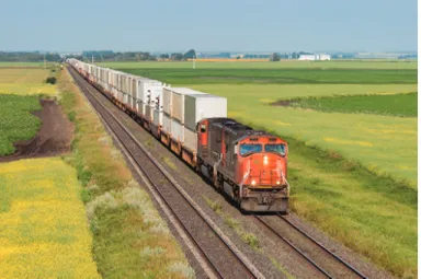
The double-stack intermodal railcar allows for roughly twice as many containers to be carried on a single railcar than a single-stack railcar. This doubling of load is critical to the efficient transportation of containers, and the growth of transportation via rail in the North American market. A train is comprised of several railcars, which are in turn comprised of platforms. Each railcar is characterized by the number and length of its platforms and by the loading patterns that determine the lengths of the containers that can be placed on each platform. A double-stack railcar has platforms on which containers can be placed on the bottom slot, and on the top slot. Platforms are defined by their length, weight, carrying capacity, as well as position in a railcar. An example of a double-stack train, loaded with containers is shown in Figure 1.1.
Figure 1.1. A double-stack train composed of several railcars, loaded with containers 1.1.3. Intermodal Container Terminals
Container terminals exist at the interface of two modes of transportation. At these locations, containers are removed from one mode of transportation, then stored or loaded directly onto another mode of transportation. The two most common types of terminals are maritime terminals, where ships interface with ground transportation, and inland terminals where containers are shifted from one mode of ground transportation to another, for example from truck to rail.
When a container is stored, it is placed in a storage yard, an area of the terminal where containers are often stacked, to some maximum height, for short term storage. A row of stacked containers is called a lot, which are generally organized by container length, such that each lot is comprised of uniform stacks. The containers in the storage area are typically organized by container destination, such that each zone of the storage area has containers going to the same destination, and as such can be loaded onto the same group of railcars. Along with the storage area, terminals have designated areas for both unloading and loading of transportation vehicles.
1.1.4. Handling Equipment
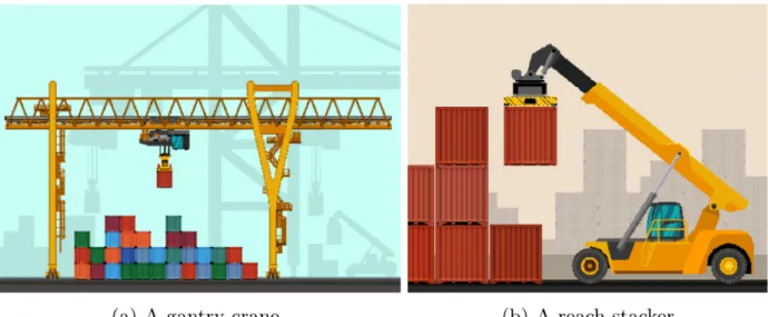
Moving containers within a terminal is done by one of two types of equipment: the gantry crane or the reach stacker, shown in Figure 1.2 and Figure 1.3 respectively. Each of these types of handling equipment is characterized by the maximum weight they can carry, as well as which containers can be reached at any given time in the storage area. Briefly, the gantry crane can lift any container off the top of any stack, while the reach stacker can only lift the top container of a stack if it is visible from the side of the storage area from which the container is being reached, and within three rows from the foremost container in that lot.
The gantry crane offers many more options for which containers can be lifted at any time. Indeed, any container that can be lifted by the reach stacker can also be lifted by a gantry crane.
Figure 1.2. A gantry crane loading a container onto a railcar
Figure 1.3. A reach stacker holding a container 1.1.5. The Load Planning and Sequencing Problem
Central to the viability of rail transportation are efficient operations at the terminals. The LPSP, first introduced by [67], is important to the operations, seeking the exact sequence and positions in which the containers will be loaded. The LPSP considers the fine details of the operations, as it addresses the handling cost, accounting for each container movement as well as wear and tear on the equipment. Generally, the objective of the LPSP is to load at minimum cost, for a given destination, as many containers as possible onto a sequence of railcars, until no more containers remain in the storage yard, or there are no more slots available on the railcars. As such, the best solutions to the LPSP are either to leave no slot unfilled while having containers remaining in the storage area, or to have no containers remaining in the storage area. The problem is defined by the layout of containers in the
storage area, the railcars available to be loaded as well as the handling equipment available to perform the loading actions.
One can consider the deterministic LPSP or the stochastic LPSP. In the deterministic case, changes to the layout of the storage area are perfectly known. Here, either containers do not arrive during the loading procedure, or containers do arrive, but the exact time of arrival and placement are known. In the stochastic case, containers can arrive during the loading procedure, and the exact time and placement of the arriving containers in the storage area are not known with certainty when the loading starts. We consider the deterministic LPSP and exclude the arrival of additional containers during loading.
1.2. Methodologies
In this section, we provide high-level background on the methodologies presented in Chapters 2 and 3 to solve the LPSP. We recall that our objective is to reformulate the LPSP that was introduced by [67] as a shortest path problem on an ordered graph. Hence, we change the solution approach from integer programming to dynamic programming. We open with an introduction to dynamic programming and follow with a brief discussion on heuristic solution methods.
1.2.1. Introduction to Dynamic Programming
We define a general deterministic sequential decision-making problem, which corresponds to a shortest path problem [7]. Time is discretized into time intervals or stages indexed by
t = 1, . . . , T . At each t, the state of the system st∈ Stis observed and an action at ∈ A(st) is
taken, incurring a cost/negative reward Gt(st,at). The terminal cost is denoted GT(sT). The
state transitions from stto st+1 according to the transition function through st+1= ft(st,at).
For a given initial state s0, the sequential decision-making problem is defined by
min a0,...,aT −1 GT(sT) + T −1 X t=0 Gt(st,at)
subject to at∈ A(st), st+1 = ft(st,at), for t = 1, . . . , T − 1. We denote an admissible policy
with π = {a0, a1, . . . , aT −1}. Further, we can define the recursive dynamic programming
equation (also called the Bellman equation) as
vt(s) = min
a∈A(s){Gt(s,a) + vt+1(ft(s,a))} , ∀s ∈ St, t = T − 1,T − 2, . . . ,0 (1.1)
with vT(s) = GT(s), ∀s ∈ ST. We also define the state-action value, the so-called Q-factor,
for a given state st and an action at following a policy π as
Due to the curse of dimensionality, it is only possible to solve (1.1) exactly for fairly small size problems. Therefore, there exist a wide range of heuristics that have been proposed in the optimal control (e.g., [7]) and reinforcement learning (e.g., [77]) literatures. While these two fields use different vocabularies, their methods have deep commonalities and a recent textbook is devoted to this topic [8]. Chapter 2 proposes algorithms rooted in the optimal control literature whereas Chapter 3 illustrates the application of an algorithm stemming from the reinforcement learning literature. In the following section, we present background on the latter. We note that we use the reinforcement learning vocabulary, but that similar techniques are described using a slightly different vocabulary in the contexts of approximate dynamic programming [64] or neuro-dynamic programming [9]. Reference [8] provides translations between reinforcement learning and optimal control vocabulary. 1.2.2. Artificial Neural Networks and Deep Reinforcement Learning
We begin by presenting a brief and high-level overview of function approximation in reinforcement learning. Next, we discuss artificial neural networks (ANNs) which are used as function approximators in DRL. Finally, we present some common techniques used in DRL.
ANNs are a common form of nonlinear function approximators. They have the property of being universal function approximators [26], which allows them to approximate any func-tion. We leverage this to have an ANN approximate the action-value funcfunc-tion. An ANN is comprised of several interconnected units which are modelled to have properties similar to neurons, a component of the nervous system. These units are organized into layers, which have linear weights, describing the strength of their connections. Additionally, each unit comprises a nonlinear activation function generating its final output. The output of unit i in layer l is defined as
ai(xl−1) = f (Wi,:l x l−1
+ bli) (1.3)
where Wl
i,: is a row of the connection weight matrix, bli is the ith bias value in the current
layer, xl−1 is the input into layer l, and f is the nonlinear activation function. This can be
repeated for each unit in the lth layer, which can act as the input into the (l + 1)th layer. The outputs of the ANN are compared with the observed labels via a loss function which measures the difference between the predicted and the target outputs. The loss function is selected depending on the type of problem being solved. For example, mean squared error loss is often used when working with scalar regression models, while cross-entropy loss is frequently used for classification models. The choice of loss function is up to the designer of the model, but it is necessary for the loss function to be differentiable, to allow for updates to be made to the weights and biases of the network. We define a loss function,
weights and biases, θ, and yj is the target output label for input xj. Consider a dataset D = {(x1,y1), (x2, y2),..., (xn, yn)}, drawn from some distribution generated by pdata. We
would like to minimize the expected loss over the underlying distribution, a value called
risk:
J∗(θ) = E(x,y)∼pdataL(f (x; θ),y), (1.4)
with respect to θ.
However, since we do not have the data generating probability distribution, pdata, the true
risk cannot be minimized, as we only have the sample D, whose empirical distribution is ˆ
pdata. Thus, we minimize the expected loss over the available dataset known as the empirical risk:
ˆ
J (θ) = E(x,y)∼ ˆpdataL(f (x; θ),y). (1.5)
In order to minimize the loss over the dataset, we update the weights and biases of each layer via backpropagation. In backpropagation, the derivative of the empirical risk over the dataset is computed with respect to each weight and bias of the ANN and these derivatives are used to update the values of the weights and biases using gradient descent as shown in (1.6).
θt+1 ← θt− ηO ˆJ (θt) (1.6)
Generally, this updating procedure is performed over minibatches of the dataset rather than the full dataset, leading to stochastic gradient descent (SGD).
Convolutional neural networks (CNNs) are specialized for working with higher-dimensional data arranged spatially, such as images [41]. While CNNs were initially designed for visible images, they have been extended to handle higher-dimensional data, for instance that generated by magnetic resonance and by computational topography in medicine, with networks based on 3-D convolutional layers. We make use of CNNs in this work to attend to the 3-D aspects of the LPSP.
Having discussed ANNs and their ability to be universal function approximators, we move on to their application in the realm of DRL. They differ in what exactly they are used to approximate, either the value function or the action-value function or both of them. In DRL, the agent interacts with the environment, creating a dataset on which the agent is trained, based on its behaviour. The objective in DRL is learning which actions an agent should take in an environment to maximize rewards. The labels in DRL are not the correct
output but a model’s approximation to the actual output based on its own experience and
parameters. Moreover, the algorithms in DRL aim to improve the reward attained by the agent, rather than just better approximate the value functions. This fundamental difference
leads to algorithms designed to maximize the expected reward that an agent will attain during the training procedure.
Learning policies in DRL can be broken into two distinct types: on-policy and off-policy learning. As described by [77], on-policy learning occurs in methods which attempt to evaluate or improve the policy which makes decisions, whereas off-policy learning occurs in methods which attempt to evaluate or improve a policy which is different from the one used to generate the data. Learning in off-policy based methods allows for the use of trajectories and data that were created following a different policy than the current one. An important characteristic of off-policy learning is sample-efficiency, since it can make use of experiences generated using a different policy from the one currently defined by the network.
In Chapter 3, we consider deep Q-learning, which uses a deep Q-network (DQN) to esti-mate the action-value function for the LPSP. The DQN is trained using an algorithm called deep Q-learning with experience replay. The idea behind the deep Q-learning algorithm is to estimate the action-value function using the Bellman equation (1.2) as an iterative update (over iterations indexed by i). In the vocabulary and notation of reinforcement learning, this is expressed as follows:
Qi+1(s,a) = E[r(s,a) + γ max a0∈A(s0)Qi(s
0
,a0)|s,a], i = iterative update (1.7) where Qi(s, a), r(s,a) and γ are respectively the Q-factor at iterate i, the observed reward
from taking action a in state s and the discount factor. Moreover, s0 and a0 are the next stage state and actions. The discount factor controls the importance of future rewards to the model. While the LPSP itself is best represented in an undiscounted environment, the discount factor can help to improve stability during training. We use r and max here rather than the previous notation to match the notation found in DRL, where the outcome from taking an action in an environment is typically called the reward, which one aims to maximize rather than minimize, in contrast to costs. Here, the action-value function is updated each step taken in the environment. Thus, the action-value function Qi+1 uses the previous
iterations action-value function, Qi, to estimate of the following state s0 and actions, A(s0).
After each step and action taken in the environment, the action-value function is updated. To do this, we sample experiences through an experience replay. Experience replay is a technique which makes use of a memory of past states, actions and rewards. Those are sampled randomly to train the network and update the parameters, thereby decorrelating the data used to train the network, and smoothing the training distribution over many past behaviours. The experience replay also discards the need to develop a probabilistic model of the system, but can lead to ovefitting to the history of the agent. Since experiences are sampled from a memory, they are likely to be generated using a model defining a different policy than the current model. As such, this method is an example of off-policy learning.
As a high-level description, we use the Q-network, Q(s,a; θ), with parameter vector θ, and calculate the loss as follows
L(θ) = Es,a∼p[(y − Q(s,a; θ))2] (1.8)
where p is a probability distribution over the behaviours saved in the experience memory. We draw from the experience memory st, at, rt, st+1, recall that st+1 = f (st, at), and define
the label using (1.7) and (1.9)
y = rt if st+1 is terminal rt+ γ maxa0Q(st+1,a0; θ) otherwise. (1.9) The following specific challenges must be met in an application of DRL: ensuring adequate exploration of the environment, managing instability during the training process, for example stemming from bootstrapping.
Chapter 2
First Article.
Heuristics for the
Load Planning and
Sequencing Problem
by
Kyle Goyette1, Emma Frejinger1, and Giancarlo Kerg2
(1) Department of Computer Science and Operations Research and CIRRELT, Université de Montréal
(2) Montréal Institute of Learning Algorithms
This article will be further revised and submitted to a yet undetermined publication.
Author Contributions
• formulation of the LPSP as a shortest path problem, • design, implementation and test of the heuristics, • definition of a lower bound and its computation,
• analysis of test results, comparisons and presentation, including writing most content of the paper.
Giancarlo Kerg contributed to the proof of the lower bound.
2.1. Introduction
Rail transportation is a critical component of intermodal transportation in North Amer-ica, providing an efficient yet flexible means to transport goods. In the U.S., intermodal rail volume has grown from 9 million containers in 2000 to 13.7 million containers in 2017. Containers accounted for 92 percent of intermodal transportation volume in 2017 according to [4], partly due to the fact that they can be double-stacked, which increases efficiency of transporting goods. While these large increases in volumes have been gained, efficient terminal operation is an important factor for this growth.
Central to intermodal rail transportation is the loading of containers onto railcars. This paper is devoted to this problem. As defined by [67], given a set of containers in a rail terminal, and a set of railcars to be loaded, one must jointly determine the assignment of containers to railcar platforms as well as a sequence of handling operations placing the containers such that the commercial value of the train is maximized and the cost of handling the containers is minimized.
Typically, the problem is divided into two separate problems, the load planning problem (LPP) and the load sequencing problem (LSP), which are solved sequentially as shown in [63]. In the LPP, a set of containers is chosen to maximize the commercial value of a train and the output is the load plan which indicates the position of each container on the train. The LSP then uses the load plan to determine a sequence of operations which minimizes the costs of handling operations when loading the containers. When solved sequentially, the solution to the joint problem can be poor. This can be alleviated by taking into account that there can be many optimal solutions to the LPP.
Double-stack intermodal railcars have only recently become a focus of research. Reference [53] proposed a model with several container and railcar types which include double-stacking railcars but specifically focus on the LPP. Reference [67] extend this work by introducing the LPSP. They solve the problem using a commercial integer linear programming (ILP) solver, but this solution approach does not scale well to large problem instances, or to problems considering the distance travelled by the handling equipment. They show that solution quality can be improved compared to a sequential solution approach.
In this work we adopt a different solution approach. We cast the LPSP as a shortest path problem on a directed graph with the aim to propose heuristics that can provide high-quality solutions to the real-size LPSP in short computing time.
The contributions of this paper are as follows:
• The deterministic LPSP for double-stack intermodal railcars is formulated as a se-quential decision-making problem.
• We propose a two-stage heuristic that combines beam search with depth-first search. It produces high-quality solutions in less than 5 minutes.
• We prove that a lower bound (LB) can be computed by solving a relaxation of the problem following a greedy policy. We leverage the LB in the proposed search heuristics.
• We compare the quality of different distance functions at approximating the true cost. The results show that considering the distance travelled in one direction provides a good approximation to the total cost.
The paper is structured as follows: the next section describes the LPSP problem. Sec-tion 2.3 provides an overview of related work. We present the formulaSec-tion in SecSec-tion 2.4. The proposed heuristics are outlined in Section 2.5. An extensive numerical study is reported in Section 2.6. Finally, Section 2.7 provides concluding remarks and outlines some directions for further research.
2.2. The Load Planning and Sequencing Problem for Double-Stack
Intermodal Trains
The LPSP is found at many container terminals and arises when one must load containers onto a vehicle. Here we focus on the LPSP found at rail terminals as described by [67]. In this problem containers are loaded onto a train and we do not explore additional complexities such as having containers off-loaded from trains or trucks during the same time period. The problem considers the handling equipment used at the terminal, the layout of the container storage in the terminal as well as the loading constraints related to the vehicle and container characteristics. In the problem, a sequence of T − 1 container movements by a single given handling equipment is selected. At each time step t < T a container is paired with a slot on a platform, or a container is double touched, which removes the container from the storage area but does not place it onto a platform.
Intermodal rail terminals are divided into several distinct areas based on their activities. An overview of the areas in a railroad container terminal is shown in Figure 2.1. Containers can arrive by truck, vessel or rail to the unloading operation area and are transferred to the storage area. Handling equipment then organizes all containers in the storage area into stacks with some maximum height. We denote the set of all containers in a problem as
C = {c1, . . . ,c|C|}. A train is composed of several railcars, R = {r1, . . . , r|R|}, which are
in turn composed of one to five platforms. We define the sequence of all platforms in the problem as P = {p1, . . . , p|P |}. Each platform has 2 slots, thus we define the set of all slots
as Q = {q1
b, qt1, . . . , q
|P |
b , q
|P |
t }, where b refers to the bottom slot, and t to the top slot, and
the numerical index refers to the platform number. When a train is ready to be loaded, containers are taken from the storage area, one at a time, by the handling equipment, h, and placed in their assigned location on the train. In the context of this paper, the side of the storage area closest to the unloading operation area is considered the back side of the storage area, while the side closest to the train operation area is considered the front side.
Figure 2.1. An overhead view of the railroad container terminal considered (taken from [67])
The retrieval of containers from the storage area is generally governed by the layout of the storage area and the handling equipment. Container placement is constrained by the placement of previous containers, the rules of placement for a given railcar, and the rules of placement for specific container types.
We consider the deterministic form of the LPSP, where the location of all containers is known, and additional containers are not placed in the storage area during the sequence of operations.
2.2.1. Retrieving Containers from the Storage Area
The storage area is a structured environment with each container’s position indicated by
containers, represented by the x coordinate in Figure 2.1. The y coordinate indicates which row the container is in, where y = 1 indicates the first row next to the train. The z coordinate indicates the vertical position of a container. Stacks in a lot are limited to a certain height, in our application three containers. We also assume that containers are sorted by their destinations into separate sections of the storage area. Hence, all containers in a single problem instance can be loaded onto the same sequence of railcars which are also assumed to be going to the same destination. We define the position of a container c as (xc, yc, zc).
We define the position of platform p as (xp, yp,0). We also define the position of platform p’s
bottom slot qb as (xqb, yqb, zqb) = (xp, yp, 1) and top slot qt as (xqt, yqt, zqt) = (xp, yp,2).
In order for a container to be retrieved, it must be accessible by the handling equipment available in the terminal. Handling equipment in railroad container terminals is generally one of two types, a gantry crane or reach stacker, both shown in Figure 2.2. Each type has its own set of rules determining which containers can be reached given a layout of containers in a storage area. For a gantry crane, the rule is simple, if the container is the top container on any given stack, it can be retrieved. However, the rules for a reach stacker are somewhat more involved.
Figure 2.2. Schematic designs of gantry cranes and reach stackers
A reach stacker retrieves containers from the storage area by lifting a container from the top while facing the container longest side. There are several rules determining when a container can be reached by a reach stacker. It is capable of lifting only a subset of the top containers and a summary of the forbidden loading operations can be found in Figure 2.3. In this figure, the blocking container must be moved prior to the selected container. Case a) is the only relevant case for the gantry crane, while cases a) through e) apply to the reach stacker. As such, the top containers of stacks closest to the back or front side of the storage area are reachable and the reach stacker is only capable of retrieving containers which are
visible from either the front or back side of the storage area. Formally, for a container c with position (xc, yc, zc) there cannot be a container c0 with xc0 = xc and zc0 = zc where yc < yc0
for the container to be reached from the front side of the storage area, or yc0 > yc to be
reached from the back side of the storage area.
The reach stacker is capable of reaching over one or two rows of containers to access a container, so long as the desired container does not exceed the maximum weight which depends on the number of rows being reached over by the reach stacker. We denote by mc
the weight of container c, θ1 the maximum container weight when reaching over one row of
containers, and θ2the maximum container weight when reaching over two rows of containers.
Figure 2.3. Summary of forbidden loading operations for a reach stacker (adapted from [67])
Given the layout of the storage area, it may be that one would like to retrieve a container that cannot be accessed without first moving another container. Moving a container without placing it onto a train is referred to as double touching and is often called reshuffling in the literature. The container that is double touched can be placed onto a platform at a later time, or left at the terminal. Since double touches entail additional costs and represent inefficiency, they should be avoided whenever possible. However, double touches are sometimes necessary, and with an appropriate allocation of cost, can be necessary to minimize the overall cost of operations at a railroad terminal.
Handling containers is a source of cost in a container terminal. One of the objectives to be minimized is the cost of handling the containers while loading a train. Handling costs account for the number of containers handled, and the distance the handling equipment must travel. As discussed previously, containers can be accessed from both the front and the back side of the storage area. When accessing containers from the back of the storage area, a reach stacker must perform a detour. In this case, the reach stacker must travel to the sides of the storage region to both lift the container, and place it on a railcar platform.
Bottom Slot
Top Slot
Platform
n
um
b
er
from
fron
t
1
2
3
4
5
1
2
3
4
5
AAR Guide
Load
capabilties
2-20’ 2-20’ 2-20’ 2-20’ 2-20’
1-40’
1-40’
1-40’
1-40’
1-40’
1-40’ 1-40’ 1-40’ 1-40’ 1-40’
1-45’
1-45’
1-45’
1-45’
1-45’
1-48’
1-48’
1-48’
1-48’
1-48’
1-53’
11-53’
11-53’
1Table 2.1. Example of an AAR Guide loading pattern
2.2.2. Assignment of Containers to Railcars
There are several factors determining which platform slots can receive containers in the solution to the LPSP. The railcar platform one may place a container onto can be restricted due to center of gravity constraints, maximum weight capacity of the platform, or load-ing patterns associated with the railcar as described in [53]. Additionally, the restrictions considered are the same as those considered in [67].
The containers found within the railroad terminal, C, are standardized containers. Each container, c ∈ C, is characterized by its length, Lc (there are five distinct lengths used in
the North American market (20-foot, 40-foot, 45-foot, 48-foot, and 53-foot), by its height,
hc and by its weight, mc. There are six types of containers defined by [53] which can restrict
where a container can be placed. However, we only consider two types here, high-cube dry containers, having a height of 9 feet 6 inches and low-cube dry containers, having a height of 8 feet 6 inches, both of which are standard six-sided containers. Finally, it is also assumed that each container has a cost associated with not being loaded on the railcar, π. Note that we do not handle 20-foot containers in our problem instances.
Intermodal trains are made up of a sequence of railcars. Each railcar r has an associated cost of use τr. An intermodal railcar is in turn made up of a number of platforms, where the
set of all platforms associated with r are denoted Pr. Each platform p ∈ P , is characterized
by its length, Lp, weight capacity, gp and tare weight, mp. A railcar is also characterized
by a set of loading patterns, which each define the lengths of possible containers that can be placed in each slot (top or bottom) for each platform on the railcar. A loading pattern can also indicate that a container of a certain length can be placed in a position, if the positions adjacent to that position are filled with containers beneath a certain length. For example, Table 2.1 shows the loading patterns for a 5-platform railcar. The railcar can accept two
153 ft container in top slot of first, third and fifth platform only when maximum 40 ft container is loaded
20-foot containers, or a 40-foot container on the bottom slots of each platform. The top slot of each platform can be filled with any container length up to 53 feet, but a 53-foot container can only be placed on the first, third and fifth platform and still can only be placed there if the adjacent top slots have a container with maximum length of 40 feet. Loading patterns restrict where a container can be placed, and in doing so make the placement of containers interconnected.
The placement of containers is also restricted by center-of-gravity (COG) restrictions imposed on the set of double-stacked containers. As regulated by the AAR, the COG of a fully loaded platform cannot exceed 98 inches at top of rail. Reference [53] provide a formulation for the maximum weight of the container occupying the top slot of a double-stacked platform, knowing the weight and height of the bottom container and the weight of the platform. The COG restriction creates another manner in which the placement of future containers is dependent on the placement of previous containers. Finally, each platform of a railcar has a maximum weight capacity, which cannot be exceeded by the sum of the weights of all containers loaded onto the platform.
In summary, the LPSP for double-stack intermodal railcars is defined with the objective of minimizing the cost of unloaded containers, unused railcars and handling of containers at the terminal. The loading depends on the location of the containers in the terminal and on restrictions governing the assignment of containers to slots on railcars (e.g., COG constraints, weight capacity of platforms and loading patterns of railcars). The solution to the problem is defined as a sequence of handling operations wherein a container is moved either directly to a given slot or is placed aside.
2.3. Related Literature
We begin by discussing the relevant literature to the LPSP for double-stack intermodal railcars and outline the differences between existing works and what is considered in this paper. The literature related to container handling problems in intermodal terminals is abundant. Here, we focus on work closely related to our problem. For a detailed overview of the related work we refer to [76, 75, 12, 13, 67]. Following this, we consider problems similar to the LPSP which are solved through dynamic programming (DP). Next, we discuss the literature addressing stochastic problems similar to the LPSP. Finally, we present studies relevant to the heuristics described in this work.
Closest to our work is that of [67] who introduce the LPSP for double-stack intermodal railcars. They compute solutions with an ILP solver with different distance functions. These distance functions approximate the cost of travel as a constant, consider the distance covered between the container and its target location, and the distance travelled in both directions, from the handling equipments current position to the container, and from the container back to the selected platform. We use the same distance functions here and these are introduced in
Section 2.4.2. As opposed to their exact solution approach, we focus on designing heuristics to solve larger instances in shorter time. Where possible, we compare our solutions with their results.
There is a rich body of literature focused on solving different kinds of operational terminal optimization problems through dynamic programming. Beam search is used by [38] to find the joint solution to the placement and load sequencing of outbound containers at port ter-minals. They focus on maximizing operational efficiency while satisfying loading constraints. The researchers propose a method using filtered beam search to determine the number of containers to select from each yard-bay and standard beam search to determine the loading sequence of the containers. Their problem differs from ours in that the representation of the ocean terminal is different from that of inland terminals which we consider.
The container load sequencing problem in ocean terminals is approached using a hybrid DP algorithm by [10]. They define the container load sequencing problem as follows: given an initial yard layout as well as a final layout of containers once loaded onto a ship, one must determine the sequence of loading operations which minimizes container relocations. Sim-ilarly, [71] consider the same problem as [10]. However they add an additional constraint, based on the crane operator’s ability to see where they are placing a container based on previously loaded containers. They propose an alternative solution using a greedy random-ized adaptive search procedure. This differs from the problem here in that the cost only considers container relocations and the final layout is given, making the problem closer to the sequential solution of the LPP and the LSP.
The container marshalling problem is formulated as a sequential decision-making problem in [31] and [32]. In this problem, a sequence of crane operations is created which selects containers and moves them to their desired location within a storage area of a container terminal. The problem aims to minimize the cost of moving containers from their initial positions in a storage area of a terminal, to one of many given desired container layouts for the storage area. Both the container load sequencing and the container marshalling problem share similarities with the LPSP: Both must determine an ordering of container movements while minimizing some handling cost and both problems are solved assuming perfect information. However, they differ fundamentally from the LPSP in that in both cases the desired location of containers is known before sequencing operations are selected. As such, they are more similar to solving the LPP and LSP sequentially as in [63].
The Ship Stowage Planning Problem (SSPP) is formulated as a sequential decision-making problem in [72]. The problem consists in optimizing the container loading sequence and assignment of containers to slots on a vessel, while respecting weight constraints. As in our problem, containers can be reshuffled (referred to as a double touch in this work). Additionally, in both the LPSP and the SSPP weight constraints can impact where containers can be placed based on previous container placement. Also, similar to the LPSP proposed
here, the problem is purely deterministic, as the layout of the containers is known, and unchanging throughout the solution. However, the two problems differ in many ways. First, the SSPP focuses purely on minimizing handling costs, which are defined by the number of times a crane must shift from yard to yard and the number of reshuffles required. In the SSPP, contraints are only dictated by the container weights.
Since some heuristics proposed in this paper rely on beam search to find solutions to the LPSP, we discuss beam search and its uses in considering container-terminal problems here. Beam search was first described by [66]. It is now often used in combinatorial optimization problems [85]. Moreover, it has been further expanded to focus specifically on combinatorial optimization problems as in [17].
State space planning is a well-explored topic in optimization and DP, wherein a search algorithm searches among states for solutions. Most state space planning methods are known as heuristic search [77]. Heuristic search allows one to better explore very large state spaces by focusing the search in regions where one expects to find a high-quality solution. Our work is an example of heuristic search, which aims to handle larger search spaces in shorter amounts of time, while dropping guarantees of optimality. Learning depth-first search (LDFS) [11], combines DFS with learning a value function. Learning is used in this sense as the defini-tion from [40] and [5], where state values are updated to make them consistent with their successors. Reference [11] presents a unified approach for heuristic search mechanisms in both deterministic and non-deterministic settings and constructs piecewise policies that be-have optimally over distinct regions of the state space. In the deterministic setting, LDFS corresponds to a variant of the A* algorithm, IDA*.
Although a number of problems related to container terminal operations have been for-mulated as sequential decision-making problems, none attend to the LPSP for double-stack intermodal railcars. We focus on this gap.
2.4. Mathematical Formulation
We begin by presenting the LPSP problem as a sequential decision-making problem that can be solved through dynamic programming. We define the states, actions and state transitions of the system. The time horizon T is discretized into a finite number of container movements indexed by t = 1, . . . , T . Next, we present three cost functions. Finally, we introduce a LB for the LPSP problem.
2.4.1. States and Actions of the LPSP
The state of the LPSP can defined as a vector s = (scpos, sd, sl, shpos) where
• scpos is a vector defined by the position of each container,
• sd is a vector indicating whether each container has been double touched,
sd = [dc∀c ∈ C]
• sl is a vector defined by whether each container has been loaded onto a platform,
sl= [lc∀c ∈ C].
• shpos is a vector defined by the positions of the handling equipment, shpos = [(xh, yh)].
The number of states grows quickly with the number of containers and platforms in the problem instance, as the number of dimensions which define the problem increase. Of course, the number of states also grows when considering the position of the handling equipment.
At each time step t of the problem, an action atcan be selected from A(st), which includes
either moving any reachable container onto any platform that does not violate constraints, or double touching any reachable container. To represent these two types of actions, we consider an action at = (c, p) to indicate moving a container c onto a platform p, and at = (c, ∅) to indicate moving a container aside. Each of these leads to deterministic state
transition functions st+1 = f (st, at). We sometimes refer to st+1 as s0.
First, let us discuss how the state transitions when a container c is placed onto a platform
p. The state here is updated by having the container position updated to that of the platform
slot, which is the same as the platform, that is: (xc,yc, zc) = (xp,yp, z). We set z = 1 when
occupying the bottom slot, and z = 2 when occupying the top slot of the platform. The slot occupied by the container is determined by the current occupancy of the platform. If the bottom slot is unoccupied, the bottom slot is filled, whereas if the bottom slot is occupied, the top slot is filled. When placing a container on a platform, all containers in the storage area previously blocked by this container become reachable by the handling equipment.
Next, let us discuss how the state transitions when a container c is double touched, defined as at= (c, ∅). Double touching a container updates the position of the container to
(xc, yc, zc) = (xc,0,0), and allows all containers previously unreachable due to container c to
be reached. Additionally, we set the double touched indicator for the container, dc= 1. Now
that the container has been double touched, it is reachable by the handling equipment from this point onward, until such point that it is placed on a platform.
2.4.2. Cost
The objective of the LPSP is to find a policy {a0, a1, . . . , aT −1) that minimizes the total
cost for a given initial state s0 defined as
G∗ = min a1,...,aT −1 T −1 X t=1 Gt(st,at) + GT(sT), (2.1)
where GT(sT) =Pc∈Cπ(1 − scl) the terminal cost incurred by unloaded containers (scl equals
cost Gt(st,at) is
Gt(st,at) = ν + γ(at)η + w(at)τr+ d(at)κ
+ [ζxDx(st, at) + ζyDy(st, at)]
+ [φxFx(st, at) + φyFy(st,at)] (2.2)
where:
• ν is the fixed cost of lifting a container.
• κ is the fixed cost of double touching a container.
• w(at) is an indicator function which takes the value 1 if a first slot is used on a railcar,
and 0 otherwise.
• τr is the cost of using railcar r.
• d(at) ∈ {0,1} is an indicator function which takes the value 1 if at time step t a
container is double touched, and 0 otherwise.
• η is the the cost of a detour to the back side of the storage area for the reach stacker. • γ(at) is an indicator variable which takes the value 1 if at time step t a detour is
taken by the reach stacker to retrieve a container from the backside of the storage area, and 0 otherwise.
• ζx and ζy are the costs of travelling with a container in the x and y direction
respec-tively.
• φx and φy are the costs of travelling without a container in the x and y direction
respectively.
• Dx(st, at) and Dy(st, at) are functions which determine the minimal Manhattan
dis-tance travelled between the container and its placement location while respecting the ability of the handling equipment to travel through the storage area.
• Fx(st, at) and Fy(st, at) are functions which determine the minimal Manhattan
dis-tance travelled between handling equipment and the container to be lifted while respecting the ability of the handling equipment to travel through the storage area. It is important to note that the difficulty of the problem depends on how we incorporate distance in the cost function. Consistent with [67], we therefore define three different cost functions which model the distance cost with increasing levels of accuracy. We present the 0-way distance function, 1-way distance function and 2-way distance function which are all special cases of (2.2). The 0-way distance function ignores distance cost, but has fixed values for double touches and detours. The 1-way distance function considers the Manhattan distance travelled from the container to its placement location, as well as adding a fixed cost for detours. Finally, the 2-way distance function considers the Manhatten distance travelled from the handling equipment’s starting position, to the container and from the container to its placement location, but does not include a fixed cost for detours. The 1-way and 2-way
Cost Function ν κ η ζx ζy φx φy
0-way distance 1 > 0 > 0 0 0 0 0 1-way distance 1 > 0 > 0 > 0 > 0 0 0 2-way distance 1 > 0 0 > 0 > 0 > 0 > 0
Table 2.2. Handling cost definition values for different distance functions
distance functions grow linearly with the distance the handling equipment must travel, while 0-way distance is a constant value depending on the container and placement location for the container. The values for travelling costs of the handling equipment and names of the cost functions are shown in Table 2.2.
The cost of leaving a container behind, π, is larger than the railcar usage cost, τr, and
is larger than the maximum handling cost when taking any action wherein a container is placed onto a platform slot.
Due to the curse of dimensionality, only small problem instances can be solved with an exact dynamic programming algorithm. We therefore propose heuristics which aim to find good solutions to the LPSP in a reasonable time frame, while sacrificing the guarantee of optimality.
2.5. Heuristics
We begin by introducing the LB for the LPSP in Section 2.5.1. In Section 2.5.2, we propose a two-stage heuristic, using beam search in the first stage to find a good initial solution. A second stage DFS improves this solution. Additionally, we present different variants of the heuristic. The search space can also be limited to a preferred action space defined using the problem structure, detailed in Section 2.5.3.
2.5.1. Calculation of a Lower Bound
The algorithms terminate once a maximum running time is reached, the space has been fully searched, or when they find a solution which meets a LB. Additionally, we compare solution values to the LB to assess their quality.
In order to compute a LB we consider a relaxed version of the LPSP that ignores both weight and length constraints of containers and railcars. In other words, any container can be placed onto any slot on any platform, so long as that slot is not occupied.
The minimum cost for the relaxed problem is achieved by minimizing handling costs while loading as many containers as possible. In short, it never reduces the total cost to leave a slot open when a container can be placed in that slot.
We demonstrate that a greedy algorithm, as shown in Algorithm 1, produces an optimal solution for all distance functions to the relaxed problem, in cases where the first lot is aligned with the first platform and lots are filled in order from the first lot along the train.
Algorithm 1 Greedy Algorithm for Calculating LB Greedy(σ(S,A))
1: G = 0
2: while σ(S,A) is not terminal do
3: gmin = ∞
% C(s) is the set of all reachable containers in state s % P (s) is the set of all unfilled platforms in state s
4: for all c ∈ C(s) do 5: for all p ∈ P (s) do 6: g = φx|xh− xc| + φy|yh− yc| + ζx|xp− xc| + ζy|yp− yc| 7: if g <= gmin then 8: gmin = g 9: amin = (c,p) 10: end if 11: end for 12: end for
13: Take action amin and observe s0,r
14: G = G + r 15: s = s0 16: end while
17: return G
Proposition 1. Let GR denote the cost of a relaxed LPSP ignoring constraints related to container and railcar properties. The cost of greedy solution πG to the relaxed problem com-puted by Algorithm 1 is a LB on the cost G∗ (2.1), GR(πG) ≤ G∗.
The proof can be found in Appendix 2.8.1. 2.5.2. A Two-stage Heuristic
We propose a two-stage hybrid heuristic search method. The first phase searches greedily among A(s) using beam search and a heuristic cost for each action. The second phase attempts to improve the solution by performing a DFS.
2.5.2.1. Phase 1: Beam Search
One can develop an order of actions to search based on the cost of retrieving and placing a container on a platform. This idea naturally leads to an implementation of beam search, wherein the cost heuristic is the immediate cost for retrieving and placing a container, and all actions that do not involve a double touch are selected with higher priority than actions wherein a container is double touched. Hence the heuristic cost used in the beam search algorithm is: Gheuristic =
Gt+ ∆ if involves a double touch
Gt otherwise,
![Figure 2.1. An overhead view of the railroad container terminal considered (taken from [67])](https://thumb-eu.123doks.com/thumbv2/123doknet/11600783.299395/32.918.119.802.361.727/figure-overhead-view-railroad-container-terminal-considered-taken.webp)