Capillary-driven shape evolution in solid-state micro- and nano-scale systems

Capillary-Driven Shape Evolution in Solid-State

Micro- and Nano-Scale Systems

by

Rachel Victoria Zucker

S.B., Materials Science and Engineering

S.B., Earth, Atmospheric, and Planetary Sciences

Massachusetts Institute of Technology, 2009

Submitted to the Department of Materials Science and Engineering

in partial fulfillment of the requirements for the degree of

Doctor of Philosophy

at the

MASSACHUSETTS INSTITUTE OF TECHNOLOGY

June 2015

c

○ Massachusetts Institute of Technology 2015. All rights reserved.

Author . . . .

Department of Materials Science and Engineering

April 13, 2015

Certified by . . . .

W. Craig Carter

POSCO Professor of Materials Science and Engineering

Thesis Supervisor

Certified by . . . .

Carl V. Thompson

Stavros Salapatas Professor of Materials Science and Engineering

Thesis Supervisor

Accepted by . . . .

Donald R. Sadoway

Chair, Department Committee on Graduate Students

Capillary-Driven Shape Evolution in Solid-State Micro- and

Nano-Scale Systems

by

Rachel Victoria Zucker

Submitted to the Department of Materials Science and Engineering on April 13, 2015, in partial fulfillment of the

requirements for the degree of Doctor of Philosophy

Abstract

Thin films are the fundamental building blocks of many micro- and nano-scale devices. However, their high surface-area-to-volume ratio makes them unstable due to excess surface free energy. Capillarity drives a process known as dewetting, during which holes form, the film edges retract, and a thickened rim of material accumulates at the edges. Various shape instabilities can occur on the film edge, resulting in complicated morphologies and break-up of the film into isolated particles. Dewetting occurs in the solid state by surface self-diffusion. In this work, a variety of models are presented to gain insights into the mechanisms that control the shape evolution of thin films. A combination of thermodynamic study, stability analyses, analytical models, explicit interface-tracking simulations, and phase-field simula-tions reveal the underlying driving forces and mass flows, explain observed morphologies and instabilities, and offer insights into how to manipulate the final structure. These pathways to control dewetting are applicable in two areas: to design micro- and nano-scale devices that are resistant to thermal degradation, and to use dewetting as a new patterning method to generate stable, complex, small-scale geometries.

Thesis Supervisor: W. Craig Carter

Title: POSCO Professor of Materials Science and Engineering Thesis Supervisor: Carl V. Thompson

Chapter 2

The calculation

of equilibrium

shapes

Chapter 3

The Rayleigh

instability on

a torus

Chapter 6

A geometric

model of the

corner instability

Chapter 8

3D iso- and

anisotropic phase

field simulations

Chapter 4

A geometric

model of edge

retraction

Chapter 7

2D fully-faceted

edge retraction

model

λ

Chapter 5

Stability analysis:

the fingering

instability

Thermodynamics

!

Simulations

!

Analytical models

!

Figure 0-1: The structure of this thesis is illustrated. The experimental images at the left of each box are from references [22, 1, 89, 47, 95, 34, 90].

Extended Abstract

Excess free surface energy exerts a driving force on materials known as capillarity. If trans-port mechanisms are active, solids can undergo shape changes to minimize their surface energy. Surface diffusion is usually the fastest capillary-driven kinetic mechanism in solids.

Substrate-supported thin films are the basic components of most micro- and nano-scale devices. However, their high surface-area-to-volume ratios equate to large capillary forces. Shape evolution by capillary-driven surface diffusion in thin films is known as “dewetting.” Dewetting is a well-known thermal degradation mechanism, but it is also gaining popularity as a patterning method.

Dewetting microstructures are distinctive, characterized by holes forming in the film, retracting edges, and a rim of material accumulating at the edges. The film undergoes either periodic pinch-off, which deposits strips of material that further break up due to a Rayleigh instability, or a shape instability, which leads to cellular or dendritic morphologies that ultimately break up into isolated particles. Prior to this work, only the simplest two shape evolution modes were understood: periodic pinch-off in isotropic materials [75, 85], and the Rayleigh instability for isotropic materials [67, 49].

In this thesis, the shape evolution modes that determine dewetting microstructures are explained and characterized. It is organized by the techniques used, which are (1) classi-cal, thermodynamic approaches, (2) analytical models of dewetting that rely on geometric simplifications, and (3) simulations that attempt to capture the full phenomenology. The sub-structure of this work is described in more detail below, and visualized in the graphical abstract, Figure 0-1.

1. Thermodynamics

The calculation and display of equilibrium shapes

The equilibrium geometry of the thin film/substrate system is the end-state of dewetting. There are two constructions available to compute equilibrium ge-ometries: the Wulff construction for isolated particles, and the Winterbottom construction for particles attached to a rigid substrate. However, these are te-dious to execute. In Chapter 2, a fast, user-friendly, open-source software tool is

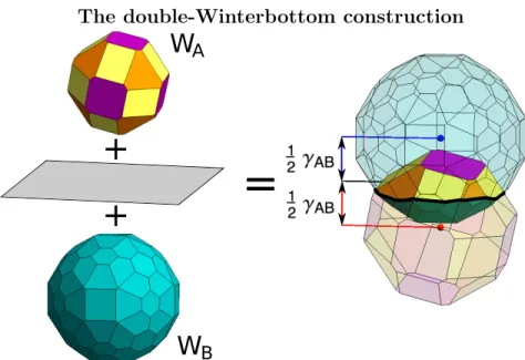
introduced to calculate and display equilibrium shapes. A new algorithm was de-veloped to accelerate the computation. In addition, a new convexification method, the “double-Winterbottom” construction, is introduced to calculate the equilib-rium geometry of a particle when the substrate mobility is not zero, as is often the case. This new class of equilibrium geometry is studied, and the double-Winterbottom method is implemented within the software tool. This work was published in the Journal of Materials Science [94].

The Rayleigh instability on a torus

The Rayleigh instability refers to the surface energy minimization-drive break-up of a cylinder of material into isolated particles. The Rayleigh instability also acts during dewetting, assisting in the break-up of strips of material. However, the strips generated by dewetting are not always straight. In Chapter 3, an exact treatment of the Rayleigh instability on a curved strip of material, i.e., a torus, is provided. The curvature is found to have a stabilizing effect. The strip’s radius of curvature must be at least four times greater than its cross-sectional radius to undergo a Rayleigh instability. When the strip evolves by surface diffusion, long-wavelength perturbations decay, in contrast to the result for a straight cylinder. A torus is found to be susceptible to an additional mode of instability, the “shrinking” instability, in which the in-plane radius decreases uniformly to reach a spherical morphology without breaking apart. The two instabilities may act simultaneously, and which one happens first depends on the aspect ratio of the torus.

2. Analytical models

A geometric model of edge retraction

The distance a film edge has retracted with time is usually fitted to a power law. However, recent numerical simulations [85, 96] have suggested that edge retraction does not follow a power-law. In Chapter 4, a simple, geometric model of edge retraction is presented that reproduces the simulation time scalings analytically. The model shows that initially, retraction is linear with time, and at late times, it approaches a power-law with 𝑡2/5 scaling. The transition time from linear to 2/5

power-law scaling is calculated as a function of contact angle. The time scalings are explained by the shape of the rim in the short and long time limits, and this model describes isotropic and anisotropic films equally well.

Stability analysis: the fingering instability

The edges of retracting thin films often undergo a shape instability. An initially-straight edge can develop finger-like projections and deposit a trail of particles behind each finger as it retracts. The “fingering instability” presents a simple means for producing nanoparticle arrays, but the cause of the instability and the factors that determine the finger spacing are unknown. In Chapter 5, a linear stability analysis on the film edge reveals the underlying cause of the instability. It is driven not by a Rayleigh-like or Mullins-Sekerka-like instability, as previously thought, but by the “divergent retraction” instability: fluctuations in rim height lead to varying retraction rates along the film edge, which grow into fingers. The analysis predicts that perturbations must have a sufficiently-large wavelength to lead to instability, and arbitrarily-long wavelength perturbations can grow. Therefore, a wide range of finger spacings are possible.

A model of the corner instability

If a film is patterned with a pre-existing polygonal hole, or if the film is anisotropic and holes are naturally polygonal, an additional shape instability is possible. The corners of holes are known to retract with constant velocity, while the edges retract at a decreasing rate [18]. This results in star-shaped holes, often with a dendritic morphology. In Chapter 6, the underlying cause of the “corner instability” is revealed using a geometric model of retraction on polygonal holes. The perimeter increase of the hole occurs entirely at the corners, and the need to lengthen the rim consumes the volume that would otherwise go into building the rim height. The rim at the corner tip reaches a stable equilibrium height, while the edges of the hole retract as usual, without interacting with the corner. The corner and edge rim height and retraction distances predicted by this simple model agree well with experiments.

3. Simulations

A 2D model of fully-faceted edge retraction

The profile of a retracting film edge has been modeled and studied before for isotropic [75, 85] and weakly-anisotropic [27] materials. In these cases, the film edge develops a thickening rim, followed by a thinning valley. However, experi-ments show that strongly-anisotropic materials do not have a valley. In Chapter 7, a model is introduced to simulate fully-faceted edge retraction. Simulations re-produce the observation that there is no valley, but visualizing the mass flows reveals slow thinning of the entire film, suggesting that the bulk of the film acts as a valley. The simulations also show that diffusivity anisotropy plays a domi-nant role in determining the rate of edge retraction. This work was published in Comptes Redus Physique [96].

A phase field simulation method for dewetting

The intermediate geometries during dewetting are usually quite complicated. Up until now, no method has been available that can simulate dewetting in 3D in a reasonable amount of time. In Chapter 8, a phase field model of dewetting, for arbitrary anisotropy, is developed and demonstrated. The phase field approach easily handles topological changes (such as hole formation and pinch-off), and the corresponding code is a finite element method including parallelization, time adaptivity, adaptive grids, implicit stabilizing terms, and a regularization scheme for handling strong anisotropy. The boundary conditions in the case of anisotropy are presented and implemented. Several test cases are shown in two and three dimensions with isotropic, weakly-anisotropic, and strongly-anisotropic surface properties.

There are five mechanisms of film break-up during dewetting: hole formation, edge retrac-tion and pinch-off, the fingering instability, the Rayleigh instability, and the corner instability. This document contains significant advances in the understanding of four of these mecha-nisms (the exception is hole formation, which cannot be explained by capillarity alone [55]). Future work includes testing the predictions of a linear edge retraction rate at early times, the

wavelength dependance for fingering and Rayleigh instabilities, and the equilibrium corner height following a corner instability, with experiments and phase field simulations.

Acknowledgments

This thesis was made possible by the commitment and generosity of countless people. Here, I wish to thank a few that have made a particularly large difference towards the occasion of completing this document, and the chapter of my life that accompanies it.

My mentor, Craig Carter, has shaped who I am as a scientist, and as a person. While I have yet to produce any work that meets his standards, they have become my standards too, and it gives me something to aspire to. Contrary to my expectations, this impossibly high bar is a source of joy, inspiration, and freshness, and it will keep me learning and growing for the rest of my life. I cannot recall doing any research with Craig, but I have nevertheless enjoyed our blunderous search for beauty in the natural world. His careful guidance has been one of the finest gifts I have ever received. I will always be indebted to him.

Carl Thompson led me to a problem that I love. His enthusiasm for discovery is infectious and absolutely delightful. To me, Carl is the quintessential materials scientist, and support from such a giant in the field gives me confidence and pride in my work. I am extremely grateful to Carl for his guidance and support.

I am indebted to Chris Schuh for his relentless encouragement. He has always pushed me to aim higher and think big. I believe in myself as much as I do now because of Chris. I also thank Jeff Grossman, who has been incredibly supportive throughout my graduate work. I am privileged to benefit from his thoughtful guidance and advice.

I have had the good fortune to find some truly exceptional collaborators. Dominique Chatain, Serge Hagege, and Uli Dahmen had a major impact on the direction of my work, and contributed to the chapter on equilibrium shapes. Alan Gye-Hyun Kim did an astonishing amount of experimental work on dewetting, and his findings underpin many of the discussions in this document. He played a particularly large role in the chapter on the corner instability. Rainer Backofen, Marco Salvalaglio, Roberto Bergamaschini, Francesco Montalentini, and Axel Voigt put in an immense amount of work in the development of the phase field code and donated many hours of computation time, and Chapter 8 would not have been possible without them. It has been, and will continue to be, a pleasure to work with these fine people. I also owe thanks to Tim Grove, who was my first mentor at MIT. His ratty t-shirts

shattered my stereotypes of professors, and he had the patience to show an 18-year-old kid what a privilege and joy it is to be a scientist. He started me on a path that has brought me a lot of joy.

The people at PICS, and more broadly in MACAN, have become my academic commu-nity, and my friends. I draw inspiration from the discussions I have had with everyone in this amazing group. Wanting to stay a part of that academic family is the strongest draw for me to stay in science.

Germany became my second home while I was a graduate student. I am grateful to Tina and Gerhard for hosting me, and to everyone in the group for making me feel welcome. I am especially thankful for Alex, for his generosity with his time, for his boundless patience to discuss and review my work, and for making me a better, more whole person.

MIT is my spiritual home. It buzzes and hums with the spastic movements of robots and nerds, and simultaneously feels like a temple, full of monks silently, patiently searching for nirvana. MIT is a state of mind, and while it is not customary to thank ideas, I can thank some of the people that made it much more palatable. Many faculty in the materials science and EAPS departments had a big impact on me, academically and personally, and I thank each and every one of my instructors for their time and efforts. The DMSE office - namely because of Angelita Mireles, Elissa Haverty, and Amy Shea - is my happy place on campus, and I am so grateful to them for always taking care of me. Kathy Fitzgerald, Jennifer Patten, and Maria Tsafoulias were incredibly generous in offering administrative support, and I am so glad their doors were always open. My friends Alan, Matt, David, Nancy, Sema, Tim, Claudia, Wenhao, Billy, Deepak, Red, Chelsea, Jennie, Andi, Olivia, Christian, David, Alison, Adrianne, Noah, Chris, Sam, and Randy always made everything better, and carried me through it all. And to say that Becky is a rock in troubled water in an understatement. She is a metric by which all others can measure their sanity, and always a source of comfort.

David Paul is a true Mensch, and I mean that in the rarest and noblest sense. His sense of humor is contagious, and he has become one of my dearest and most valued friends. My time as a graduate student would be hollow without our weekly lunches.

training around. Surviving a dinner conversation with that lot is intellectual jiu-jitzu. In stark contrast, my mother taught me how to think deeply, slowly, and carefully. I cannot thank her enough for sharing this dying art, and for always, always being on my side. My father is my longest-serving teacher. He taught me the scientific method with his gentle guidance and endless patience for the question "dad, why...?" Aaron is my sparring partner, and the only person that can reliably make me laugh so hard I cry. Lisa has a staggering social intelligence and insightfulness that I am only just beginning to learn from, and Joe has taught me all I know about ethics. I love you all, and my huge, ridiculous family is my most prized “possession.” I count my lucky stars every day, and every person in my family is one of them.

Contents

1 Introduction 29

1.1 The capillary force . . . 29

1.2 Thermodynamics of Interfaces . . . 30

1.3 Equilibirum shapes . . . 32

1.3.1 Isolated particles: the Wulff construction . . . 32

1.3.2 Particles Attached to a Planar Substrate: The Winterbottom Con-struction . . . 34

1.4 Capillarity far from equilibrium . . . 36

1.4.1 The kinetics of capillary-driven surface diffusion . . . 37

1.4.2 Thin films . . . 38

1.4.3 Dewetting phenomenology . . . 39

1.5 Scope of this work . . . 43

2 The Calculation and Display of Interfacial-Energy Minimizing Shapes 45 2.1 Introduction . . . 45

2.1.1 A rigorous approach to finding the equilibrium shape . . . 46

2.1.2 Isolated Particles in Homogeneous Environments: Wulff Shapes . . . 47

2.1.3 Particles Attached to Deformable Interfaces . . . 48

2.2 Methods: The Wulffmaker Software Suite and the Double-Winterbottom Method 49 2.2.1 Wulffmaker for Wulff and Winterbottom Shapes . . . 49

2.2.2 Double-Winterbottom Construction . . . 51

2.2.3 Wulffmaker for Double-Winterbottom Shapes . . . 57

2.3.1 The Equivalent Wetting Angle . . . 58

2.3.2 Contact Area . . . 59

2.3.3 Wrinkles and the Limitations of Wulffmaker . . . 60

2.3.4 Calculating interface energies from the equilibrium shape . . . 63

2.3.5 Allowed and Non-Physical Morphologies . . . 64

2.3.6 Consequences of Anisotropy on the Wetting of Interfaces . . . 68

2.4 Conclusions . . . 68

3 The stability of a torus under capillary forces 71 3.1 Introduction . . . 71

3.1.1 Review of the Rayleigh instability on a cylinder . . . 72

3.2 The stability of a torus against capillary forces . . . 73

3.2.1 Geometry . . . 73

3.2.2 Possible perturbation wavenumbers . . . 73

3.2.3 Longitudinal perturbations . . . 74

3.2.4 Other perturbations . . . 76

3.3 The fastest-growing perturbation on a torus . . . 77

3.3.1 The Rayleigh instability . . . 77

3.3.2 The shrinking instability . . . 82

3.4 Conclusions . . . 83

4 A 2D analytical model of dewetting 85 4.1 Introduction . . . 85

4.1.1 Basis for comparison: Brandon & Bradshaw’s method applied to a straight edge . . . 86

4.2 Model development . . . 88

4.2.1 Geometry and assumptions . . . 88

4.2.2 The retraction velocity as a function of rim height . . . 89

4.2.3 The rim height as a function of time . . . 90

4.2.4 The retraction distance as a function of time . . . 91

4.3.1 Limiting behavior . . . 92

4.3.2 Comparison with numerical simulations . . . 94

4.4 Conclusions . . . 95

5 The Fingering Instability: a Stability Analysis of Retracting Thin Film Edges 97 5.1 Introduction . . . 97

5.2 Possible mechanisms of the fingering instability . . . 97

5.2.1 Rayleigh-like instability . . . 98

5.2.2 Divergent retraction instability . . . 99

5.2.3 Arc length instability . . . 99

5.2.4 The combined effect of the three instabilities . . . 101

5.3 Methods . . . 102

5.3.1 Geometry and assumptions . . . 102

5.3.2 The triple line perturbation growth rate, GRTL . . . 103

5.3.3 The rim height perturbation growth rate, GRRH . . . 105

5.3.4 The perturbation growth rates for the three instabilities . . . 108

5.4 Results and discussion . . . 109

5.4.1 Properties of the perturbation growth rate . . . 109

5.4.2 The contributions of the three instabilities . . . 112

5.4.3 Discussion . . . 118

5.4.4 Comparison with other models and experiments . . . 118

5.5 Conclusion . . . 119

6 The Corner Instability: An Analytical Model and Underlying Mechanisms121 6.1 Introducion . . . 121

6.2 Summary of experimental results . . . 122

6.3 Corner instability model . . . 124

6.3.1 Model geometry . . . 125

6.3.2 Retraction velocity . . . 127

6.3.4 The steady-state rim height at the tip . . . 131

6.4 Discussion . . . 133

6.4.1 The mechanism of the corner instability . . . 133

6.4.2 Evidence against other mechanisms for the instability . . . 133

6.4.3 Comparison of the model and experimental results . . . 134

6.5 Conclusion . . . 136

7 A 2D model for dewetting of a fully-faceted thin film 139 7.1 Introduction . . . 139

7.2 Model implementation . . . 141

7.3 Reference film . . . 143

7.4 Results and discussion . . . 144

7.4.1 Reference film retraction . . . 144

7.4.2 Numerical sensitivity . . . 145

7.4.3 The influence of film parameters on the rate of retraction . . . 145

7.4.4 Comparison with experiments . . . 154

7.4.5 Pinch-off . . . 154

7.4.6 Valley formation . . . 155

7.5 Summary and conclusions . . . 156

8 A phase field model for dewetting 159 8.1 Introduction . . . 159

8.2 Phase-field formulation for dewetting . . . 160

8.2.1 Isotropic equations of motion . . . 160

8.2.2 Isotropic boundary conditions . . . 163

8.2.3 Anisotropic regularization . . . 164

8.2.4 Anisotropic equations of motion . . . 165

8.2.5 Anisotropic dewetting boundary condition . . . 166

8.3 Numerical method . . . 169

8.3.1 Challenges . . . 169

8.3.3 Computation . . . 171

8.4 Results and Discussion . . . 171

8.4.1 Limitations of the phase field approach . . . 176

8.5 Conclusions . . . 177

9 Conclusions 179 9.1 Edge retraction and valley formation . . . 180

9.2 Film edge instabilities . . . 181

List of Figures

0-1 Graphical abstract . . . 6 1-1 The effect of surface curvature on excess free energy . . . 30 1-2 The weighted mean curvature and dE/dV . . . 32 1-3 The Wulff construction . . . 33 1-4 The Winterbottom construction . . . 36 1-5 Experiments showing incomplete dewetting morphologies . . . 40 1-6 Isotropic edge retraction . . . 41 1-7 The fingering instability . . . 42 1-8 The corner instability . . . 43 2-1 The new convexification algorithm . . . 52 2-2 The Wulffmaker user interface . . . 53 2-3 The double-Winterbottom construction . . . 54 2-4 The double-Winterbottom method and the energetic description of wetting . 56 2-5 The effect of orientation of the contact angle . . . 59 2-6 The influence of contact angle on particle geometry . . . 60 2-7 Wrinkles and the double-Winterbottom construction . . . 62 2-8 The influence of interfacial energy on the triple line shape . . . 63 2-9 Comparison of real and modeled double-Wintrebottom particles . . . 65 2-10 Possible double-Winterbottom morphologies . . . 67 2-11 Interface orientation and the contact angle . . . 69 3-1 The torus geometry . . . 73

3-2 The stability field for a torus . . . 76 3-3 The shape changes of a torus due to surface diffusion . . . 79 3-4 Top-down views of perturbed torii with surface diffusion . . . 80 3-5 The surface velocities used in the analysis . . . 80 3-6 The perturbation growth rates for a torus under surface diffusion . . . 81 3-7 A stability map for a torus under surface diffusion . . . 82 3-8 The shrinking instability . . . 83 4-1 The assumed cross-sectional profile of the film edge . . . 89 4-2 The retraction distance versus time . . . 92 4-3 The transition time from linear to power-law retraction . . . 93 4-4 The limiting behavior of edge retraction versus time . . . 94 4-5 A comparison between this model and numerical simulations . . . 95 5-1 A schematic of the fingering instability . . . 98 5-2 The three mechanisms of instability . . . 100 5-3 The assumed geometry of the rim . . . 103 5-4 The geometry for the volume conservation calculation . . . 107 5-5 The perturbation growth rates . . . 110 5-6 Perturbation growth rates in the long-wavelength limit . . . 111 5-7 The critical and fastest-growing wavelengths . . . 113 5-8 The influence of rim height on perturbation growth . . . 114 5-9 The perturbation growth rates for the three underlying instabilities and the

fingering instability for different 𝜃 . . . 116 5-10 The perturbation growth rates for the three underlying instabilities and the

fingering instability for different 𝜖 . . . 117 6-1 Experimental study of the corner instability . . . 123 6-2 A schematic of the corner geometry . . . 126 6-3 The arc length coordinates . . . 128 6-4 The discretized time evolution of the corner tip . . . 130

6-5 Stability of the corner tip . . . 132 6-6 Comparison of model and experimental results . . . 135 7-1 Reference equilibrium shapes . . . 144 7-2 The retraction of an anisotropic film edge with time . . . 144 7-3 Time scalings of an anisotropic retracting film edge . . . 145 7-4 The effect of diffusivity on edge retraction . . . 146 7-5 The effect of each facet on edge retraction . . . 147 7-6 The chemical potential and mass flux on the film edge . . . 148 7-7 The effect of surface energy on edge retraction . . . 150 7-8 The effect of contact angle on edge retraction . . . 152 7-9 The effect of film thickness on edge retraction . . . 152 7-10 Pinch-off due to bulk film thinning . . . 155 7-11 The rate of bulk film thinning . . . 156 7-12 Anisotropic edge retraction with a faceting instability on the top surface . . 157 8-1 Topological changes in phase field versus explicit interface models . . . 160 8-2 The dewetting boundary condition in a phase field . . . 164 8-3 𝛾, 𝜉, and the anisotropic phase field boundary condition . . . 167 8-4 An anisotropic equilibrium shape calculated with phase field in 3D . . . 172 8-5 The triple line at equilibrium . . . 173 8-6 Phase field simulation of the fingering instability . . . 174 8-7 Phase field simulation of the Rayleigh instability . . . 175 8-8 Rim profiles with different Wulff shapes . . . 175 8-9 Phase field simulation of a faceting instability . . . 176

List of Tables

7.1 The diffusivity on each facet and fit parameters for the curves in Figure 7-4 . 147 7.2 The diffusivity on each facet and fit parameters for the curves in Figure 7-5 . 149 7.3 The 𝑐𝑡𝑛 fit parameters for each curve in Figure 7-7 . . . 150

Chapter 1

Introduction

1.1

The capillary force

Surface tension, or capillarity, is familiar when dealing with liquids. The capillary force holds drops of liquid together, creates the meniscus line in a container, and is responsible for “capillary action;” that is, the ability of a liquid to climb up a narrow channel, even in opposition to external forces like gravity. Capillarity acts on solids as well. At macroscopic length scales, there are few visible effects of surface tension in solids. However, at the micro-and nano-scales, capillarity can be the largest driving force acting on a system micro-and dominate its dynamics.

Capillarity is chemical in origin. It can be explained two ways: either as a pressure, or as an excess free energy. As a pressure, it originates from the attractive bonds between atoms or molecules in a condensed phase. For example, water molecules interact via hydrogen bonds, which holds a water or ice droplet together. The water molecules in the center have neighboring molecules in all directions, so the net force is zero. However, the water molecules on the surface only have neighbors on one side, generating a pressure that compresses the droplet. As an energy, it originates from the unsatisfied bonds of the surface molecules. For example, consider a material that has minimum energy when it has twelve nearest-neighbors, such as an FCC crystal. At the surface, only six nearest-neighbor bonds are possible. The six remaining unsatisfied bonds increase the free energy of the surface atom. Therefore, one might expect the surface energy density of this material to be six times

The effect of surface curvature on excess free energy

Positive

curvature

Negative

curvature

Flat

Highest

energy

Low

energy

Lowest energy = bulk

High

energy

Figure 1-1: A schematic shows the effect of curvature on excess surface free energy. Atoms are shaded by their energy, using a Lennard-Jones pair potential. An atom in the bulk of this material has 8 bonds. An atom at the surface has less than 8 bonds, but the number depends on the surface curvature.

the bond energy, divided by the surface area per atom (the square of the bond length). This bond-breaking estimation of the surface energy density is crude, but it gives a decent approximation (e.g., [81]).

1.2

Thermodynamics of Interfaces

The bond-breaking explanation of capillarity is useful for understanding its dependance on surface curvature. If a normally 8-coordinated material is cut along a plane, the average number of unsatisfied bonds is exactly 3, as shown in Figure 1-1. However, if the surface of the material is corrugated, the average number of unsatisfied bonds varies. For an atom sitting on top of a hill, there are more than 3 unsatisfied bonds. For an atom sitting in a valley, the number of unsatisfied bonds is less than 3.

Consider the change in energy of the system in Figure 1-1 upon adding an atom to the surface. The change in energy will depend on where the atom is placed. If the change in energy upon adding an atom to an infinite, flat surface is defined to be zero, then the energy will increase if the atom is placed on top of a hill, and decrease if it is placed in a valley. This

is the reason that the chemical potential of a surface is proportional to the mean curvature, 𝐾. For capillarity, the chemical potential along a surface, 𝜇, relative to an infinite, flat surface, is [32]

𝜇 = 𝛾𝐾Ω, (1.1)

where 𝛾 is the surface energy density of the material, and Ω is the atomic volume. Because a pure material is being considered, the chemical potential refers to single species and 𝜇 can be related to the local vapor pressure. The mean curvature 𝐾 is a geometric property defined as 𝐾 = 1/2(𝐾1 + 𝐾2), where 𝐾1 and 𝐾2 are the principal curvatures of the surface. If 𝑟1

and 𝑟2 are the principal radii of curvature on the surface, then 𝐾 = 1/2(1/𝑟1+ 1/𝑟2). Mean

curvature is a measure of how quickly the surface area 𝐴 changes if the interface moves and sweeps through some volume 𝑉 : 𝐾 = 𝑑𝐴/𝑑𝑉 .

The total energy of an interface is ∫︀_𝐴𝛾𝑑𝐴, where 𝐴 is the total interfacial area, 𝑑𝐴 is a surface element, and 𝛾 is the surface energy density of the material. In the isotropic case, 𝛾 is independent of the surface orientation, so it can be moved outside the integral, and the total energy is 𝛾𝐴. If the material is anisotropic, 𝛾 is a function of surface orientation, and must remain inside the integrand.

Anisotropic materials have a surface energy density that depends on the interface orien-tation, 𝛾(𝑛), where 𝑛 is the surface normal. In the extreme case of a fully-faceted material, the isotropic definition of chemical potential becomes meaningless because the facets have zero mean curvature, except at the corners, where the mean curvature is undefined. The chemical potential is instead written in terms of the more general weighted mean curvature, or WMC, 𝜅𝛾 [77]:

𝜇 = 𝜅𝛾Ω. (1.2)

The physical meaning of chemical potential can be used to obtain an expression for WMC. The chemical potential for a pure material is the change in total energy upon the addition of material, 𝑑𝐸/𝑑𝑁 , where 𝑁 is the number of atoms. 𝑑𝐸/𝑑𝑁 is equal to Ω 𝑑𝐸/𝑑𝑉 . Figure 1-2 shows 𝑑𝐸/𝑑𝑉 for three cases of a fully-faceted geometry. The additional volume is shaded light blue, and the change in length of facets on the shape are highlighted. The change in total surface energy, divided by the volume added, is the WMC, 𝑑𝐸/𝑑𝑉 .

The weighted mean curvature and dE/dV

Figure 1-2: The change in length caused by moving a facet outwards along its normal, for three types of facet. Facets are labeled in gray, and their normal vectors are drawn in black. (a) A regular facet, which has positive WMC (weighted-mean curvature) and 𝜎 = 1. Outward motion causes the total length of the facet to decrease. (b) A neutral facet, with zero WMC and 𝜎 = 0. Outward motion causes no net change in the length of the facet. (c) An inverse facet, which has negative WMC and 𝜎 = −1. Outward motion causes the total length of the facet to increase. (Figure after [77].)

In the isotropic limit, WMC reduces to the surface energy times mean curvature, 𝛾𝐾. For fully-faceted 2D geometries, it can be shown that the WMC of the 𝑖𝑡ℎ facet on a polygon is [77]

𝜅𝛾_𝑖 = 𝜎Λ𝑖 𝐿𝑖

(1.3) where 𝜎𝑖 is 1 if the facet is regular, 0 if the facet is neutral, and -1 if the facet is inverse (see

Figure 1-2 for explanations of regular, neutral, and inverse), 𝐿𝑖 is the length of the facet,

and Λ𝑖 is a geometric factor, given by

Λ𝑖 = 𝛾𝑖+1− 𝑛𝑖· 𝑛𝑖+1𝛾𝑖 √︀1 − (𝑛𝑖· 𝑛𝑖+1)2 + 𝛾𝑖−1− 𝑛𝑖· 𝑛𝑖−1𝛾𝑖 √︀1 − (𝑛𝑖· 𝑛𝑖−1)2 , (1.4)

where 𝑖 + 1 indicates the next facet, 𝑖 − 1 is the previous facet, and 𝑛𝑖 is the normal vector of

the facet [77]. This expression can be calculated from Figure 1-2. The geometric factor is also identical to the length of the facet with the same orientation on the equilibrium shape [77].

1.3

Equilibirum shapes

1.3.1

Isolated particles: the Wulff construction

When the only contribution to excess free energy is interfacial energy and the volume is fixed, the equilibrium shape of an isolated particle in a homogeneous environment is the Wulff

The Wulff construction 1. Surface energy plot

θ

γ(θ)

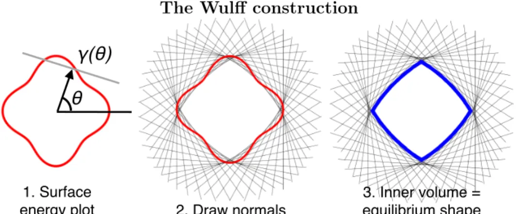
Figure 1-3: The Wulff construction is demonstrated for a two-dimensional material. The Wulff construction begins with a plot of 𝑛 𝛾(𝑛) for all 𝑛 on the unit sphere, where 𝑛 is the normal vector to a surface, and 𝛾(𝑛) is the interfacial energy of that surface. For all orientations, a plane perpendicular to 𝑛 is drawn a distance 𝛾(𝑛) from the origin. All points on the far side of the plane are discarded. The remaining volume is the equilibrium shape, or Wulff shape.

shape [86]. For isotropic materials, the Wulff shape is a sphere because this minimizes the total area. For anisotropic materials, there is a competition between two effects: a sphere has the minimum area, but a polyhedron with facets corresponding to the lowest energy orientations avoids the higher energy orientations. The equilibrium shape is a compromise between these two extremes.

The equilibrium shape can be found using the Wulff construction [86] (Figure 1-3). The Wulff construction is performed on the interfacial energy density −→𝛾 (ˆ𝑛) ≡ |−→𝛾 (ˆ𝑛)|ˆ𝑛 = ˆ𝑛𝛾(ˆ𝑛), where −→𝛾 is a vector function of all possible interface orientations ˆ𝑛 and 𝛾(ˆ𝑛) (n.b., with no vector notation) is the magnitude of −→𝛾 in the direction ˆ𝑛. An orientation, ˆ𝑛, may not be a stable interface orientation: stability is determined by whether it is removed by the Wulff construction.

To generate the Wulff shape, one begins with the plot of ˆ𝑛𝛾(ˆ𝑛). For each orientation ˆ𝑛𝑖,

a plane perpendicular to ˆ𝑛𝛾(ˆ𝑛) is drawn. This perpendicular plane divides space, and all points on the far side of the plane are discarded. After this exclusion procedure is repeated for all orientations, the remaining volume is the Wulff shape, 𝒲. The Wulff construction can be stated concisely as 𝒲 = {−→𝑝 ∈ 𝛾-space|−→𝑝 · ˆ𝑛 ≤ 𝛾(ˆ𝑛)}, where −→𝑝 are points in 𝒲-space. Because the shapes in 𝛾-space (i.e., the space in which the 𝛾-plot is drawn—where coordinates have units of energy/area) and real space are the same, the Wulff construction

can be written in real space as 𝒲 = {−→𝑥 ∈ ℜ3_|−→_{𝑝 · ˆ𝑛 ≤ 𝛾(ˆ𝑛)} with an additional constraint on}

the particle’s volume 𝑉particle =∫︀ 𝑑3−→𝑥 . The Wulff shape is always convex, and if facets are

present, all facets have 𝜎 = 1. The chemical potential is uniform at equilibrium, so WMC is constant on the Wulff shape.

There is an analogy between unstable interfacial orientations and the unstable chemical compositions in a miscibility gap [10]. The Wulff construction is a convexification of ˆ𝑛𝛾(ˆ𝑛) (|ˆ𝑛| = 1) which results in the removal of unstable orientations from the final shape, just as the common-tangent construction is a convexification of the molar free energy 𝐺(𝑋1, 𝑋2, . . . 𝑋𝑛)

(𝑋1+ 𝑋2+ . . . 𝑋𝑛 = 1) which removes unstable compositions from the phase diagram. When

a material phase separates into two distinct compositions, it does so because a mixture of the two phases has lower energy than the original composition. When an orientation separates into a collection of two or more orientations, e.g. sharp “hills-and-valleys” or “pyramids”, it does so because the total energy per projected surface area is less than that of the orientation. Such unstable orientations do not appear on the Wulff shape—they disband into 𝒲-edges for “hill-and-valley” morphologies, and disband into 𝒲-corners for pyramid morphologies.

To continue the analogy to phase diagrams, the familiar phase-diagram is a representation of the stable compositions (𝑋1, 𝑋2, . . . , 𝑋𝑁), and 𝒲 is the orientation-diagram for a physical,

tangible, shape [12]. When ˆ𝑛𝛾(ˆ𝑛) has sufficiently strong anisotropy, 𝒲 is composed of planar facets, which are analogous to line-compounds. Whereas line-compounds occur at special stoichiometries, the facets appear at all crystallographically-equivalent special orientations. Smooth or partially-faceted 𝒲 occur for weaker anisotropy; these also have phase diagram analogies.

1.3.2

Particles Attached to a Planar Substrate: The

Winterbot-tom Construction

The Wulff construction only applies to isolated particles in homogeneous environments. However, in many contexts of practical importance (e.g., solid-state dewetting, catalysis, micropatterned surfaces, pores in a sintered body), a particle can be attached to one or more interfaces. The equilibrium shape must minimize the sum of each total interfacial

energy while maintaining other constraints, such as particle volume and connectivity of the interfaces. The simplest example is a deformable particle with a fixed volume that abuts a non-deformable (rigid) planar interface (e.g., a liquid drop on an inert solid planar surface). In addition to the interfacial energy between the particle and its environment in the absence of the substrate (𝛾𝑃 𝑉, where V refers to the environment, which is often a vapor phase),

there are two additional interfacial energies: the interface where the substrate abuts the par-ticle (𝛾𝑆𝑃) and where the substrate is not in contact with the particle (𝛾𝑆𝑉). The isotropic

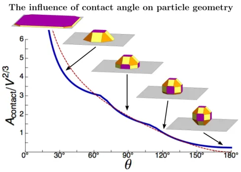
particle case is familiar: minimization produces a spherical cap that intersects the substrate with a uniform wetting angle, 𝜃, for the particle on the substrate, with

𝜃 = cos−1 𝛾𝑆𝑉 − 𝛾𝑆𝑃 𝛾𝑃 𝑉

. (1.5)

Equation 1.5 is known as the Young equation, and can be interpreted as a force balance or as a boundary condition that derives from global energy minimization—these interpretations are not independent [14]. The Young Equation is independent of particle size (in the absence of other defect energies), but the curvature of the spherical cap is determined by the particle volume. Considering the geometry of the shape in 𝒲-space, the center of the spherical gamma surface for the particle/exterior interface (with radius 𝛾𝑃 𝑉) sits a distance (𝛾𝑆𝑉−𝛾𝑆𝑃)

above the substrate. If (𝛾𝑆𝑉−𝛾𝑆𝑃) is negative, then most of the sphere is discarded, and only

a small cap remains. This is the Winterbottom construction for an isotropic particle [83].

The Young equation is helpful in determining the equilibrium shape of an isotropic par-ticle, but it is not obvious how it pertains to a general anisotropic particle. Winterbottom showed that the 𝛾 = 0 point will be a distance (𝛾𝑆𝑉 − 𝛾𝑆𝑃) above the substrate not only

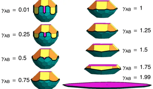
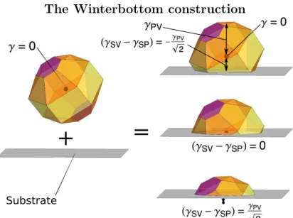
for isotropic particles, but for a particle with a general Wulff shape [83]. Additionally, the selection of the 𝛾 = 0 point is known to be arbitrary [46]. An example of the Winterbot-tom construction with various (𝛾𝑆𝑉 − 𝛾𝑆𝑃) values is shown in Figure 1-4. The case when

(𝛾𝑆𝑉 − 𝛾𝑆𝑃) is positive is often referred to as “bad wetting,” while the case when (𝛾𝑆𝑉 − 𝛾𝑆𝑃)

The Winterbottom construction

=

Substrate

+

Figure 1-4: Left: the Winterbottom construction begins with the Wulff shape of a particle and (𝛾𝑆𝑉 − 𝛾𝑆𝑃). Right: the distance between the 𝛾 = 0 point in the Wulff shape and the

substrate surface is equal to (𝛾𝑆𝑉 − 𝛾𝑆𝑃). Top: the equivalent wetting angle, 𝜃, is 135∘.

Middle: 90∘. Bottom: 45∘.

1.4

Capillarity far from equilibrium

For a body of material that is not in the equilibrium shape, there will be a difference in chemical potential across its surface. If a kinetic mechanism is available, the gradient in chemical potential will drive mass to flow from high to low WMC positions. The shape will evolve towards the equilibrium shape by a pathway determined by the fastest kinetic process available.

It is necessary to identify the dominant (fastest) transport mechanism to describe the shape evolution. In a solid, there are four possible kinetic pathways: volume diffusion, surface diffusion, evaporation-condensation, and viscous flow. All of these are thermally-activated, so shape changes due to capillarity are measurable only at homologous temperatures above about 0.5 [32]. Herring showed that capillarity does not drive viscous flow in crystalline ma-terials, so viscous flow can be eliminated (though it is possible in amorphous materials) [33]. For most materials, surface diffusion is orders of magnitude faster than volume diffusion, so volume diffusion can be eliminated as well. Finally, Mullins calculated that surface dif-fusion dominates over evaporation-condensation for crystalline materials with moderate or low vapor pressures [54]. This prediction has been verified experimentally, as the kinetics

of capillary-driven shape changes in crystalline materials which do not evaporate away over the course of annealing are consistent only with surface diffusion [78].

In the rare case that evaporation-condensation is the dominant mechanism, the mathe-matical description is much simpler than for surface diffusion, and it can be studied fairly easily [54, 15]. However, the simpler mathematics means that the morphological evolution is simple as well [15]. The rich morphological variety resulting from motion by surface diffusion (discussed in Section 1.4.3) makes it a much more exciting topic for investigation.

1.4.1

The kinetics of capillary-driven surface diffusion

To describe the motion of a two-dimensional surface, the arc length 𝑠 is used to define the position on the surface. The normal vector, 𝑛(𝑠, 𝑡), gives the orientation of the surface as a function of position and time. By convention, the normal vector points outwards, away from the material. The speed of outward motion of the interface parallel to the surface normal, 𝑉𝑛, as a function of time and position, gives the complete evolution.

Mullins developed an expression for 𝑉𝑛(𝑠, 𝑡) for isotropic materials undergoing

capillary-driven surface diffusion [54]. His derivation began with the chemical potential (𝜇(𝑠, 𝑡) = 𝐾(𝑠, 𝑡)𝛾Ω), discussed in Section 1.2. The flux of surface atoms in response to curvature gradients is given by Fick’s first law:

𝐽 (𝑠, 𝑡) = −𝐷𝑠𝜈

𝑘𝑇 ∇𝑠𝜇(𝑠, 𝑡) = −

𝐷𝑠𝛾Ω𝜈

𝑘𝑇 ∇𝑠𝐾(𝑠, 𝑡), (1.6)

where 𝐷𝑠 is the surface self-diffusivity, 𝜈 is the surface concentration of mobile atoms, 𝑘 is

Boltzmann’s constant, 𝑇 is temperature, and ∇𝑠 is the Laplace-Beltrami operator, i.e., the

gradient operator restricted to the surface profile [54]. Physically, Fick’s first law states that when a gradient in potential is present, material tends to flow down that gradient to lower the total energy.

If the flux is locally divergent, then mass is leaving that location and the surface height is decreasing. Likewise, if the flux is convergent, the surface height is increasing, and it has a positive velocity along its normal. Thus, the surface velocity along its normal, 𝑉𝑛(𝑠, 𝑡), is

minus the divergence of the flux: 𝑉𝑛(𝑠, 𝑡) = 𝐷𝑠𝛾Ω2𝜈 𝑘𝑇 ∇ 2 𝑠𝐾(𝑠, 𝑡), (1.7)

where the extra factor of Ω is included to convert the units to a velocity [54]. This governing equation can be generalized to include anisotropy [93, 15]. The result is much less readable, but the derivation is the same.

The material constants in Equation 1.7 can be collected into a single material property, 𝐵 = (𝐷𝑠𝛾Ω2𝜈)/(𝑘𝑇 ). The governing equation can be non-dimensionalized using 𝐵 (units of

length4/time) and a characteristic length scale 𝐿:

𝑣𝑛(𝑠, 𝑡) = ∇2𝑠𝜅(𝑠, 𝑡), (1.8)

where 𝑣𝑛 is the dimensionless normal velocity, 𝑣𝑛 = 𝑉𝑛𝐿4/𝐵, and 𝜅 is the dimensionless

mean curvature, 𝜅 = 𝐾𝐿.

1.4.2

Thin films

Although capillary forces affect material of all shapes and sizes, in this work, special attention is given to solid thin films. This is for two reasons: first, thin films are the basic building blocks of most micro- and nano-scale devices, so they are of technological relevance, and second, thin films have large aspect ratios (width/thickness), so they are especially unstable with respect to capillarity. Large aspect ratios mean large surface-area-to-volume ratios, so the excess surface energy is high, thus the capillary driving forces are high.

We define a “thin film” as any material body supported by a substrate with a characteristic thickness 𝐿. The shape of the thin film in the plane of the substrate may be simple or quite complicated, e.g. as a result of patterning with lithography. The presence of the substrate has a profound effect on the shape evolution because it provides an additional constraint (i.e., maintaining contact with the substrate).

The process of capillary-driven shape evolution in thin films is called “dewetting.” The end state of dewetting is an array of isolated particles, each having the equilibrium shape.

De-pending on the materials and starting geometry, the particles may be randomly-distributed, or ordered. Nanoparticle and quantum dot arrays are in demand for a variety of applications, and dewetting provides a simple method to make them. Dewetting has been used to generate particle arrays for optical and magnetic devices [3, 65], sensors [50, 3], catalysis [19, 64, 57], nanowire growth [70, 21, 92, 20], and memory devices [17, 65]. These applications mo-tivate investigations to understand how to control the particle arrangements produced by dewetting.

The intermediate stages of dewetting include a huge variety of morphologies. An example of incomplete dewetting is reproduced from Ye et al. [90] in Figure 1-5. When anisotropic films are patterned via lithography and then dewetted, reproducible, complex structures with sub-lithographic feature sizes are produced. Possible features include isolated particles, wire-like lines of material, which may be interconnected, and unaffected film. Devices with components made by partial dewetting should be much more thermally stable than equivalent devices made by conventional methods. This is because the components are already partially equilibrated, so the driving force for motion is dramatically lower.

1.4.3

Dewetting phenomenology

Dewetting is a well-known phenomenon, and it has been studied extensively [78]. Dewetting has four main morphological features: edge retraction, the growth of rims, hole formation, and break-up into islands of material.

Dewetting is mostly localized at film edges. This is because the gradients in surface curvature, and therefore driving forces, are largest near the edge. Edges bound the as-deposited film, or they can be the result of post-deposition patterning, or they can form spontaneously when a film is heated and holes form by natural processes. As an example of the latter, grain boundary grooves in polycrystalline films can extend through the entire thickness of the film and nucleate holes [38, 74].

Once edges are present, they will retract to reduce the film’s surface area. Retraction is facilitated by a mass flux from the receding triple line (the intersection of the film/vapor, vapor/substrate, and substrate/film interfaces) to the advancing side of the rim [96]. An edge with an initially-square profile will evolve toward a shape with uniform WMC and

Experiments showing incomplete dewetting morphologies

Figure 1-5: This figure shows a variety of starting geometries (dashed lines) and the corre-sponding incomplete dewetting morphology. This image is reproduced from Ye et al. [90]. The view is top-down, dark gray is the substrate, and light gray is the film material. Each subfigure corresponds to a unique starting condition, and the resulting film pattern is repro-ducible. The black scale bar is 10 micrometers.

Isotropic edge retraction film substrate mass flux rim retraction direction

Figure 1-6: During isotropic dewetting, the initially-flat film forms the equilibrium contact angle with the substrate, the corner rounds, and the triple line retracts. Mass accumulation at the film edge generates a rim, and a valley follows.

forms the equilibrium contact angle at the triple line [75, 85]. A thickened rim develops on the edge due to mass accumulation, as shown in Figure 1-6. The thickening rim also lowers the WMC, so the edge retraction rate decreases with time.

As a film edge retracts, a valley may form ahead of the moving rim [75, 85, 27]. Relative to the bulk film height, the valley is roughly an order of magnitude smaller in depth than the rim is tall [75, 85]. As the rim grows, the valley deepens. In no other process interferes, the valley eventually touches the substrate, pinching-off a strip of material, and the cycle begins again with quick adjustment to the equilibrium contact angle, formation of a new rim, and ultimately another pinch-off event [85]. The cyclic formation of valleys and pinch-off has been seen experimentally [88].

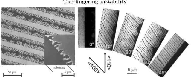
However, pinch-off is not always observed. The “fingering instability” may instead dom-inate the dewetting morphology (see Figure 1-7). This instability is observed in both poly-crystalline [37, 38, 53] and single-crystal films [24, 29, 47], and is characterized by growing variations in triple line position and rim height, which eventually develop into an array of protruding fingers. The fingers may undergo a Rayleigh instability [67], as shown on the right in Figure 1-7, and deposit a trail of isolated particles. The spacing and width of the fingers primarily determines the spacing of particles produced via dewetting. Knowledge of the parameters which govern the length scale of break-up can therefore be used to control

The fingering instability

Figure 1-7: Fingering instabilities in polycrystalline Au (left) and single-crystal Si (right) are shown. The images are reproduced from Jiran & Thompson [38] and Leroy et al. [47].

structures resulting from via dewetting.

Anisotropic single-crystal films exhibit additional features. They are strongly affected by the crystallographic alignment of the film [24, 89, 60, 76, 29], and edges with different in-plane crystallographic orientations retract at different rates [89, 8]. If the equilibrium shape is composed of flat facets connected by rounded corners, numerical simulations give a rim-and-valley film edge profile [27]. However, when the equilibrium shape is composed exclusively of flat facets with sharp corners, no valley is expected [43]. An absence of valleys is observed for fully-faceted single-crystal Si films [27, 8], Au-Fe films [43], and for some edge orientations in Ni films [34].

Strongly-anisotropic films have edges which are composed of facets. These edges have minimum retraction rates. If a film is patterned with an edge that is not kinetically-stable, it may decompose into stable facets and develop a “staircase” morphology [89]. This break-up is referred to as a “faceting instability.”

Strongly-anisotropic films develop polygonal holes bounded by kinetically-stable facets. After the initial stages of growth, the corners are observed to retract faster than the centers of the edges. This is typically referred to as the “corner instability,” and leads to dendritic or star-shaped holes [88, 89, 63, 60, 7, 76, 29, 18, 8], as shown in Figure 1-8. Kinetic Monte Carlo simulations of dewetting in single-crystal structures also exhibit corner instabilities [61, 8].

The corner instability

Figure 1-8: Corner instabilities in various materials are shown. The figure is reproduced from the review by Thompson [78], and the sub-figures are from references [76, 60, 29, 7].

1.5

Scope of this work

Although much of the relevant thermodynamic and kinetic framework to describe dewetting has already been developed, many of the mechanisms which govern dewetting remain un-known. Some of the outstanding fundamental questions in capillary-driven surface diffusion are presented in the following chapters, and resolved using advancements in thermodynamic theory (chapters 2 & 3), the development of new analytical models (chapters 4-6), and the development and application of new simulation techniques (chapters 7 & 8). The last chapter discusses broader conclusions about dewetting that can be drawn from this work.

Chapter 2

The Calculation and Display of

Interfacial-Energy Minimizing Shapes

2.1

Introduction

To study capillary-driven shape changes, it is essential to know the equilibrium configuration of the system. The equilibrium state defines the direction of evolution. The Wulff construc-tion and Winterbottom construcconstruc-tion, introduced in Chapter 1, are approaches to compute the equilibrium shape. However, these constructions are tedious. Having a software tool to do the computation would be advantageous during investigations of dewetting.

There is an additional equilibrium configuration which is relevant in capillary-driven motion. If the substrate is deformable, rather than rigid, a constraint on the interface shape is removed. “Deformable” does not refer to the mechanism by which the system achieves equilibrium, but to the freedom to take the shape which satisfies the energy minimization. For the deformable substrate case, there is no previously known construction.

In this chapter, we present a fast, conceptually simple, analytical method for finding equilibrium morphologies and energies of particles on deformable boundaries, and discuss the possible morphologies and their consequences for microstructures. In addition, a public-domain software suite, Wulffmaker, is developed to enable fast and easy display of equi-librium shapes. A discussion of allowed and non-physical morphologies is aided by these computational tools, and their utility for interpreting real data is demonstrated.

2.1.1

A rigorous approach to finding the equilibrium shape

The equilibrium thermodynamics of interfaces has been formulated by Cahn [9]. He presents a general method of expressing measurable interfacial properties in terms of derivatives of the free energy with respect to the system’s independent variables. Cahn’s formulation parallels that of Gibbs in that it begins with the interface’s differential contribution to the total system energy: 𝛾𝑑𝐴. The interfacial tension is a function of the system’s independent variables (for example, 𝛾(𝑇, 𝑃, 𝜇𝑖, . . .) and this choice of independent system variables 𝑇, 𝑃, 𝜇𝑖

is used below). In elementary treatments, 𝛾 does not depend on total interfacial area, 𝐴. The equilibrium values of each phase’s entropy, volume, and composition are completely determined by the potentials (𝑇, 𝑃, 𝜇𝑖), and their values within each phase are determined

by a convexity condition on the total free energy. This condition applies when there are no constraints on inter-phase exchange of such extensive quantities. However, if the volume of one phase is fixed, a pressure difference develops at the interface of the constrained phase— for isotropic fluid/fluid interfaces, this produces an interface of constant mean curvature. This homogeneous constant mean curvature is a result of minimization and appears as a force balance. A concrete example follows: consider an isolated soap bubble with a fixed volume. Total energy minimization results in a spherical bubble and the pressure difference is 2𝛾/𝑅. If the soap bubble is in contact with a rigid surface, minimization produces a uniform mean curvature and a boundary condition on the dihedral angle at contact [14].

The interface adopts a local composition, entropy density, and volume which are inter-nal quantities—that is, they are completely determined by the system’s (𝜇𝑖, 𝑇, 𝑃 ). For a

fluid/fluid interface, its area is also an internal variable which is determined by minimiza-tion. For solid/fluid and solid/solid interfaces, additional variables arise. When atoms are prevented from moving from the bulk to the interface, a surface stress occurs. Surface stress is addressed by Weissmüller [82]. When one of the phases is crystalline (or a liquid crystal), 𝛾𝑑𝐴 generalizes to −→𝜉 𝑑−→𝐴 where 𝑑−→𝐴 includes variation of the interfacial area |−→𝐴 | and the variation of the local surface normal ˆ𝑛 (−→𝐴 = |−→𝐴 |ˆ𝑛). In this case, the capillarity vector, −

→

𝜉 (𝑝, 𝑇, 𝜇𝑖, ˆ𝑛), depends on orientation, which is an “internal” interfacial variable.

the system’s internal geometry is often easier to compute by convexification of 𝛾. This con-vexification produces the well-known Wulff construction, which always has uniform weighted mean curvature as indicated by minimization with a volume constraint [77]. Convexification is also the proof for the Winterbottom construction [41], and it is the method used in the following sections to demonstrate the “double-Winterbottom” construction for deformable interfaces.

2.1.2

Isolated Particles in Homogeneous Environments: Wulff Shapes

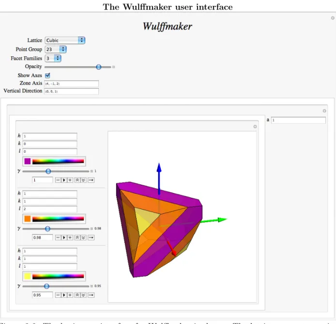
The Wulff construction can become cumbersome in three dimensions because the number of computations necessary grows with the cube of the number of ˆ𝑛’s included. Roosen, McCormack, and Carter developed the public domain software Wulffman for the general calculation of Wulff shapes [68]. Their method relies on techniques from computational geometry that are dramatically faster than the Wulff construction. Although Wulffman is powerful, fast, and versatile, it has not been supported since 2002 and only runs on Linux operating systems. This paper introduces new software, Wulffmaker, that is distributed as Wolfram Mathematica code and as a .cdf, and runs on all platforms. Wolfram now distributes a free visualizer for interactive Computable-Document-Format (cdf) files.

For anisotropic particles, there is distinction between the geometrical contact angle be-tween the particle and the substrate, 𝛼, and the equivalent wetting angle, 𝜃, which appears in the Young equation. 𝛼 is determined by the facets available on the Wulff shape and their inclinations with respect to the substrate, and can only take on discrete values for a fully-faceted particle. 𝛼 is a local property because it also varies along the triple line as different facets of the Wulff shape are traversed. On the other hand, 𝜃 can take any value between 0∘ and 180∘, and encapsulates information about the relative magnitudes of the three interface energies present. 𝜃 is defined via the Young equation (see Section 1.3). The appropriate definition of each 𝛾 term that determines 𝜃 is clear for isotropic particles, but the equiva-lent 𝛾𝑃 𝑉 (i.e., considering its multiple values and arbitrary crystallographic orientation) is

ambiguous in the case of anisotropic particles. This ambiguity is resolved in the discussion, below.

2.1.3

Particles Attached to Deformable Interfaces

Particles often nucleate at pre-existing defects to eliminate some of the associated defect energy. It is quite common to observe a minor phase in a multiphase system, such as precipitate particles in an alloy, attaching to grain boundaries in the major phase. In this case, the equilibrium shape is more complicated because the particle can distort the boundary and the triple line is not confined to a plane. A similar case occurs when particles of a distinct phase are deposited on a soft substrate, such as when a patterned thin film is annealed at a temperature high enough to allow diffusion in the substrate. The particles can become partially submerged in the substrate to create substrate-particle interface at the expense of particle-environment interface (e.g., [16]). These two cases are examples of particles attached to deformable boundaries, and represent morphologies that occur in technological applications.

To date, no simple method has be demonstrated to find the equilibrium shape of such particles. A Winterbottom-like truncation construction was demonstrated by Cahn and Hoff-mann for isotropic or symmetric and twinned particles, but they did not address a means to solve for general geometries [13]. The truncation method was proven in two dimensions [45], and has been applied in two dimensions by overlaying the appropriate Wulff shapes to ex-plain particle morphology [39]. However, the truncation method has not been discussed nor proven in three dimensions. Siem and coworkers presented a general numerical method to find these shapes, but its implementation is impractical and offers little insight into the nature of these geometries [72, 73].

The global stability of a particle attached to an interface is determined by the energy of the wetting particle compared to the energy of the particle in bulk. Methods to calculate the energy of such particles would enable an anisotropic model of heterogeneous nucleation, as well provide insight into Zener pinning for anisotropic particles.

2.2

Methods: The Wulffmaker Software Suite and the

Double-Winterbottom Method

In order to calculate equilibrium shapes, software tools were developed to quickly and eas-ily generate Wulff shapes, Winterbottom shapes, and the shapes of particles attached to deformable interfaces, which we call double-Winterbottom shapes. New, fast computa-tional methods to generate Wulff and Winterbottom shapes are developed and implemented in Wulffmaker. A general method for the construction of double-Winterbottom shapes is needed, so a new algorithm was developed and implemented in the Wulffmaker suite. These tools run in Wolfram Mathematica 8 or later versions, and are platform-independent. Wulffmaker also runs in Wolfram CDF Player, which is free and available for download: <http://www.wolfram.com/cdf-player/>. The code for these software tools and installation instructions are available online at <pruffle.mit.edu/wulffmaker>.

2.2.1

Wulffmaker for Wulff and Winterbottom Shapes

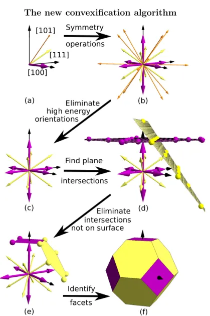
Wulffmaker employs a new algorithm to quickly generate Wulff shapes. When 𝒲 is com-pletely faceted, the computation becomes discrete and finite. In this case, the normal vectors for each facet, ˆ𝑛𝑖, and their corresponding interface energies, 𝛾𝑖, are used to construct the

Wulff shape (Figure 2-1a). The set of ˆ𝑛𝛾(ˆ𝑛) from which 𝒲 is computed has repeated values (i.e., 𝛾𝑖(ˆ𝑛𝑖) = 𝛾𝑗(ˆ𝑛𝑗) = . . . = 𝛾𝑚(ˆ𝑛𝑚)) when symmetry requires equivalence of several

direc-tions (i.e., ˆ𝑛𝑖 ∼ ˆ𝑛𝑗 ∼ . . . ∼ ˆ𝑛𝑚 where −→𝑎 ∼

− →

𝑏 implies that there is a symmetry operation that maps −→𝑎 to −→𝑏 ). The user interface is greatly simplified by utilizing this symmetry so that only one normal and one 𝛾 need be specified for all equivalent facets. However, the code computes 𝒲 by using all of the ˆ𝑛𝛾(ˆ𝑛). Symmetrically-equivalent ˆ𝑛𝛾(ˆ𝑛) are generated by applying each symmetry operation allowed for the specified point group by the following process on the initial set of generating {ˆ𝑛𝑖𝛾(ˆ𝑛𝑖)}:

1. Iteratively apply each symmetry operation to each member of the set 2. Add the results of each above operation to the set

4. Repeat 1-3 until the set stops changing.

The result of such an operation is shown in Figure 2-1(b).

Some of the generated {ˆ𝑛𝑖𝛾(ˆ𝑛𝑖)} may have such high energy that they do not appear

on the Wulff shape. The Wulff construction requires that the projection of any vector −→𝑥𝑖

from the origin to the surface of 𝒲 onto any other such vector −→𝑥𝑗 is shorter than −→𝑥𝑗.

Therefore, if the projection of a gamma vector ˆ𝑛𝑖𝛾(ˆ𝑛𝑖) onto another gamma vector ˆ𝑛𝑗𝛾(ˆ𝑛𝑗)

is longer than ˆ𝑛𝑗𝛾(ˆ𝑛𝑗) itself, then ˆ𝑛𝑖𝛾(ˆ𝑛𝑖) does not appear on the Wulff shape, and it can be

eliminated from the remainder of the calculation. Additionally, if ˆ𝑛𝑖𝛾(ˆ𝑛𝑖) is eliminated, then

all symmetrically-equivalent gamma vectors must also be eliminated. Therefore, only one member of each set of symmetrically-equivalent vectors undergoes the projection test against all other gamma vectors, and if it fails even once, the entire set of symmetric equivalents are eliminated. The result of this rapid elimination procedure is shown in Figure 2-1(c).

The elimination procedure provides the final list of gamma vectors that correspond to facets on the Wulff shape. Each gamma vector defines a facet plane with ˆ𝑛𝑖 and a distance to

the origin 𝛾𝑖. The vertices defining 𝒲 are where three facet planes intersect, and the edges

of 𝒲 are where two facet planes intersect. Therefore, 𝒲 can be found by calculating all of the points where three facets on the Wulff shape intersect, and selecting only those that fall on the surface of 𝒲 (using the same elimination procedure as above). The vertices on the surface are always generated by adjacent, or nearest-neighbor, gamma vectors. The nearest neighbor metric is defined by the projection of other ˆ𝑛𝛾(ˆ𝑛) onto the vector in question. To reduce the number of vertices that must be calculated, a list of nearby gamma vectors is assembled for each ˆ𝑛𝑖𝛾(ˆ𝑛𝑖). The intersection points of each facet plane 𝑖 with its neighbors

are calculated and tagged with the identities of the three facet planes that generated it. All of the intersection points generated from two example facet planes are shown in Figure 2-1(d). The elimination procedure applied to remove ˆ𝑛𝛾(ˆ𝑛)’s that are too large also works for the elimination of intersection points that do not appear on the surface of 𝒲. Each intersection point is projected onto the nearby gamma vectors, and if the projection is longer than the gamma vector, that point is eliminated. The remaining points define the Wulff shape, as shown in Figure 2-1(e).