Deep structure resistivity measurements in Massachusetts

-I

SEP 20 1960

LIBRA?," DEEP STRUCTURE RESISTIVITY

MEASUREMENTS IN MASSACHUSETTS by

ANTHONY M. HAUCK, III A.B., Dartmouth College

(1952)

Gp.E., Colorado School of Mines

(1958)

SUBMITTED IN PARTIAL FULFILLMENT OF THE REQUIREMENTS FOR THE DEGREE OF

MASTER OF SCIENCE at the

MASSACHUSETTS INSTITUTE OF TECHNOLOGY September, 1960

Signature of Author

Department of Geology'and Gebphysics, August 22, 190

J A

Certified by

Accepted by

/7 1 /

Thesis Supervisor

DEEP STRUCTURE RESISTIVITY MEASUREMENTS IN MASSACHUSETTS by

ANTHONY M. HAUCK, III

Submitted to the Department of Geology and Geophysics on August 22, 1960 in partial fulfillment of the requirements

for the degree of Master of Science. ABSTRACT

The thesis is an investigation of the apparent resistivity of rocks below the earth's surface.in Massachusetts. Field measurements were obtained for two continuous profiles, 10 and 11 miles in length, along the Massachusetts Turnpike between

Framingham Center and Millbury and between Auburn and Sturbridge, respectively. One-mile-long sending and receiving dipoles were used, with dipole separations up to

6

miles. Subsurface

apparent resistivity values are compared to and correlated with those of surface samples measured in the laboratory.

In order to establish the validity of apparent resistivity values obtained along the Turnpike profiles, in particular for a 5-mile-long conducting zone east of Sturbridge, the possible effects of guardrails and the boxwire fence bordering the

Turnpike upon the electrical dipole field are considered.

Guardrail and fence contact resistances were small, indicating that both the guardrail and fence could have distorted the

electrical field. In a field experiment the apparent resistivity when the receiving electrodes were 70 feet from the fence was 7% less than that obtained when the electrodes were 10 feet from the fence. However, this variation was probably not within the accuracy permitted by the instrumentation. Laboratory model work indicates that at most the presence of the fence would be to decrease the apparent resistivity values by 50-55%. It is concluded that the low apparent resistivity values in the zone east of Sturbridge were caused by the presence of disseminated graphite and sulfides in the country rock.

In 1934 Slichter published an electrical potential map of the eastern part of Massachusetts covering an area about 50 miles in diameter centering at Clinton. Dipole and monopole apparent resistivity contour maps were prepared from Slichter's potential map and are compared with the Geologic Map of

Massa-chusetts and with the apparent resistivity profiles along the Massachusetts Turnpike. Comparison indicates a maximum of 8000-10,000 ohm-meters apparent resistivity at the deepest

depths permitted by the dipole separations, and does not indicate a continued increase in apparent resistivity with depth.

Thesis Supervisor: T. R. Madden

Assistant Professor of Geophysics

ACKNOWLEDGEMENTS

The author wishes to particularly express his gratitude to Professor Theodore Madden, who suggested and supervised the thesis investigation, for his continued guidance and

criticism. He is indebted also to Professor Thomas Cantwell, who made all the arrangements necessary in obtaining

per-mission to conduct field work along the Massachusetts Turnpike, for his advice and suggestions throughout the investigation.

The gathering of resistivity field data on such a large scale necessarily requires the combined efforts and cooperation of a number of people. In addition to Professors Madden and Cantwell, who gave freely of their time for the

field work, the author wishes to express gratitude to Neil Dulaney, Charles Racer, William Thompson, Duane Uhri, and Eugene Perry, all graduate students in the Department of Geology and Geophysics, for their help and interest. Since traffic conditions along the Turnpike prohibited working on weekends, it was often necessary for the above individuals to be absent from their classes.

The author is also indebted to Emanuel Bombolakis of the Department of Geology and Geophysics for corroborating the rock sample identifications.

The Massachusetts Turnpike Authority entered into an indemnity agreement with the Massachusetts Institute of Technology and granted members of the Department of Geology and Geophysics permission to conduct field work along the Turnpike.

iv

Support for the field investigation came from the National Science Foundation's Grant NSF-G6606 to Professor Madden. The same grant made possible a half-time research assistantship for the author during the second semester of the academic year 1959-1960.

TABLE OF CONTENTS

Page

ABSTRACT . . ... ... 1

ACKNOWLEDGEMENTS . . . . . . . . . . . . . . . . . .iii

CHAPTER I . . . . . . . . . . 1

1.0 Purpose and Introduction . . . . . .. . . . . . . 1

1.1 Field Procedure. 0 . .. .. . . . .. 2

1.2 Field Instrumentation . . . . . . . . . . . . 5

1.j Measurement Sites . . . - - - . . . 5

1.4 Laboratory Apparent Resistivity Measurements . . . 7

1.5 Presentation and Discussion of Field Results . . . 9

1.6 Guardrail and Fence Contact Resistance Measurements . 15 1.7 Field Model Experiment . . . . . .. 17

1.8 Laboratory Model Study . . . .. . . .. . . . . . . 19

CHAPTER _II . . . . . . . . . . . . . . . . . . . . 28

2.0 Discussion of Slichter's Work . .. . . . . . . . 28

2.1 _{Calculations Made from Slichter's Data . . . . . ..;30}

2.2 Discussion of Slichter's Potential Map . . . . .

59

2.5 Discussion of Dipole Apparent Resistivity Contour Map . . . .6 . . . . .0 41 2.4 _{Discussion of Monopole Apparent Resistivity Contour} Map _{. . . . . .*}

₄₄

2.5 _{Discussion of Apparent Resistivity Values from} Slichter's Data in Light of Turnpike Field Results . 49 CHAPTER III . . . - - - * * - - - . . 56

Page

TABLES

I. Description of Rock Samples Taken along Massachusetts

Turnpike . . . .. . . . 59

II. Laboratory Apparent Resistivity Measurements . . . . 61

APPENDICES

I. Derivation of Apparent Resistivity Formula for a

Half Space . . . . - - . 64

II. Method of Weighting Monopole and Dipole Distances. .

66

FIGURES

1 Location Map . . . - - - - . - - - - 6

2 Apparent Resistivity Measurements along Massachusetts

Turnpike, Framingham Center-Millbury . . . 10

5

Apparent Resistivity Measurements along Massachusetts

Turnpike, Auburn-Sturbridge . . . 11

4 Contoured Apparent Resistivity along Massachusetts

Turnpike . . . - 12

5 R.M.S. Volts versus Frequency for 0.02" Diameter

Rod . . . 21

6 Percent of No-Rod Voltage versus Rod Distance from

Electrodes . . . . . 23

7 Rod Diameter versus Rod Distance from Electrodes . . 25

8 Copy of Slichter's Potential Map . . . 29

9 Apparent Resistivity Dipoles . . . 51

10 Apparent Resistivity Monopoles . . . . . 32

11 Apparent Resistivity versus Distance from Clinton

Electrode . . . . . . . . . . . . . . . . . * 54

vii

Page

15 Apparent Resistivity versus Weighted Distance from

Sending Dipole (Pittsfield Potential: 0.6 mv/amp) . 7 14 Apparent Resistivity versus Weighted Distance from

Sending Dipole (Pittsfield Potential:

3.25

mv/amp) . 58

15 Contour Map of Dipole Apparent Resistivity

(film positive) . . . . . . . . . . . . ... . . 46

16 Contour Map of Monopole Apparent Resistivity

(film positive). . . . 47

17 Copy of Emerson's Geologic Map of Massachusetts

-1916 . . . . .s.i. v e r s u 48

18 Apparent Resistivity versus Weighted Distance for

Dipoles . . . 51

19 Apparent Resistivity versus weighted Distance for

Monopoles. . .

53

- I - _ - , _ _ --,-,- -Q i _ -.- _ I - -- -. ,- !- -V __

CHAPTER I

1.0 Purpose and Introduction. 1

The purpose of this investigation was to obtain apparent resistivity measurements in the upper regions of the earth's crust in Massachusetts that would serve as a check on results obtained by concurrent magneto-telluric work at M.I.T.

Areas bordering the Massachusetts Turnpike were chosen as measuring sites because they conveniently provided l0-to-15 mile long strips that were virtually free from electrical

interference and at the same time cut across the regional geologic structure.

During the course of the investigation it became apparent that the guardrails and boxwire fence which border the Turnpike could be factors affecting the field apparent resistivity

results, particularly where they were continuous for large distances. In an effort to determine their possible effects, laboratory measurements on rock samples taken along the Turn-pike, measurements of contact resistances in the field, and field and laboratory model studies were performed.

In the early stages of the investigation Slichter's (1934) work was brought to attention via a personal communication

between Professors Slichter and Madden. Calculations were made on the basis of Slichter's data with the intention of comparing them with the results of the field data taken along the Turnpike and with values at greater depths obtained by the magneto-telluric methods (see Cantwell, 1960).

1.1 Field Procedure.

The sending and receiving system used in the field was the so-called modified Eltran array or dipole-dipole configu-ration, and is described by both Hallof (1957) and Ness (1959). The procedure was to fix the position of the receiving circuit while moving the source along the line in the same direction.

S R

2 3 8 8 : 9:

S-2 etc.

R-4 S = source dipole position

S-1 S-2 R = receiver dipole position

R-4 R-5

dipole length = 1 mile

The receiving arrangement consisted of one and two-mile

lengths of wire so that signals could be received consecutively on four one-mile dipoles. The sending procedure was to send on one-mile dipoles on either side of a sending position, (S) in the figure above, and then to move on to another sending position.

The data was plotted below the surface line, as shown above, at the intersections of 45-degree lines drawn from the middle of the particular sending and receiving dipoles. This method has the advantage of lending a two-dimensional character

1.2 Field Instrumentation.

A. Sending Equipment:

The sending equipment was powered by a gasoline-driven, 400 cps-115 volt, A.C. generator, and is illustrated in the following schematic:

Trons- ConstaintOu t

Genera~tor -+ + 10re Rectifier -+- Curren- -+b hopper

Oscillator

Circuit

The D.C. output was calibrated to 0.5 cps by means of a Sanborn Recorder in the laboratory, and this frequency was used throughout the field measurements. Cantwell's (1960)

measurements at a number of localities in Massachusetts showed a telluric current low at 1 cps, but skin effect considerations and the fact that the resonan-t frequency of the galvonometer in the receiving system was 1 cps made 0.5 cps a better choice.

Each sending electrode consisted of a

symmetrically-arranged array of six sheets of aluminum foil, each sheet one-and-one-half feet in length, buried six inches below the ground. These were connected together by ten-foot clip leads and were wet thoroughly by a saturated salt solution. A capfull of

solution in order to enhance the contact between the earth and foil and to inhibit oxidation of the foil. Electrodes planted in this manner were found to perform satisfactorily four days after they had been planted.

The contact resistance of a sending dipole made up of two such electrodes was about 500 ohms. Number 26 coated magnet wire was used for the sending dipoles. During the field measurements ground conditions permitted sending a current ranging from 200 to 700 milliamperes.

B. Receiving Equipment:

The receiving equipment used in the field measurements was essentially the same as that used by Cantwell (1960) for his telluric current measurements, and may be illustrated in

the following schematic:

Varimble,

Banc-W Pass FilIter-s

0 Low- Pass

4 Filter Amprifitx

A gasoline-driven, 60 cps-115 volt generator was used as the power supply for the amplifier and filters. The receiving electrodes were porous ceramic pots filled with copper sulfate solution. A copper rod with one end immersed in the copper sulfate served as a connection to the receiving dipole wire. Number 28 coated magnet wire was used for the two-mile

electrode connections mentioned previously. Contact resistances for the receiving dipoles ranged from 2000 to 4000 ohms.

5

The incoming 0.5 cps signal was read as peak-to-peak voltage on the galvonometer, and was easily distinguished visually from the longer period telluric current drift.

Signal amplitudes ranged from 100 microvolts to 40 millivolts. It was necessary to amplify the incoming signal 1000 times for the largest distances (five and six miles) in between a sending and receiving dipole.

1.j Measurement Sites.

Sites used for field measurements and at which surface samples were taken were from mile markers No. 109 to No. 99 along the northern side of the Massachusetts Turnpike between the Framingham Center and Millbury Exits, and from mile markers No. 90 to No. 79 between the Auburn and Sturbridge Exits.

These are indicated by the hachured areas in Fig. 1 and are labeled I and II, respectively.

An attempt was made to make field measurements west of the Connecticut River from mile markers No. 40 to No. )5 between the Westfield and Lee Exits along the southern side of the

Turnpike. Surface samples were also taken in this area, which is not shown in Fig. 1.

LOCATION MAP Pepperell' Tyngsboro Greenfield Gardner Littleton Common 'Concord T] so/t*n Barre _Clinton Rutland Wv. Boy/s Holden Northboro Shrewsbury N BrooAfield Wvorceste'r

Westboro-Leicester* Upton Miford Scale OF Miles 'mitinsvile 05/0 /5 * Auburn 'Oxford kWebs ter hayland 'Frarnin 9ham .Cooleyville .Grafton

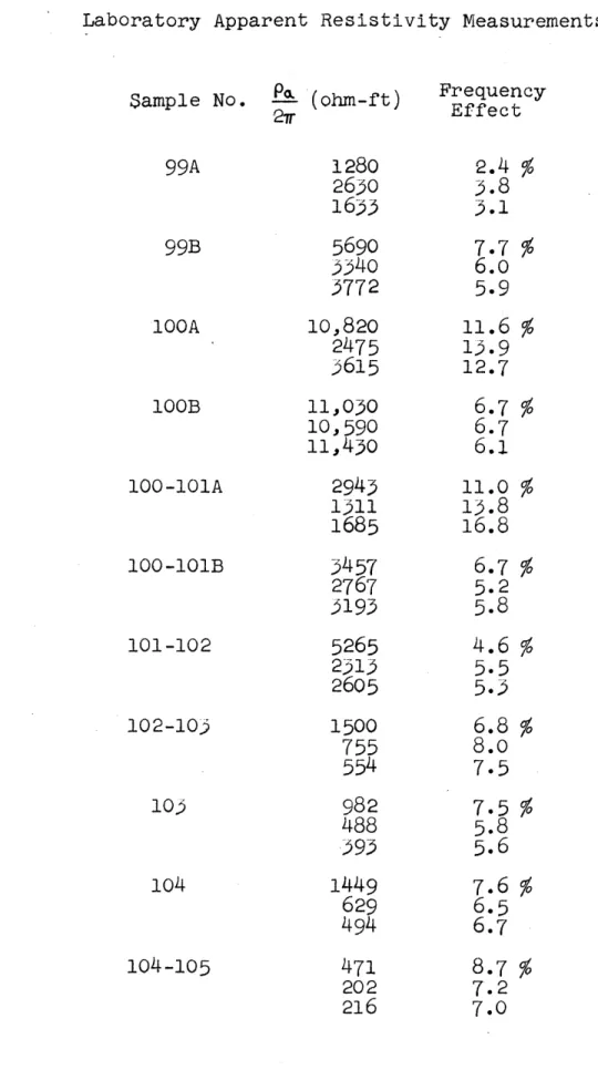
1.4 Laboratory Apparent Resistivity Measurements.

7

The apparatus used for measuring the rock sample apparent resistivities in the laboratory is described in detail by

Madden and Marshall (1958 and 1959). A general block diagram of the apparatus is shown below (feedback circuits are omitted).

Triggerin3 Relaj Re.ILag0410

C

ircui t

Circuit

- -S m e -+-

Circuit

- - scofe

The samples were immersed in tap water for at least two days prior to the measurements. Electrical contact with a sample was made by two pairs of silver gauze electrodes coated with AgCl, separated from the sample and from each other by thicknesses of tap-water-saturated felt.

Direct voltages were read on the oscilloscope and used to calculate the apparent resistivity of a two-inch-cube sample in three mutually perpendicular directions. In addition to the apparent resistivities the induced polarization frequency effect at 10 cps and a delay time of 0.01 sec. was measured

in the three directions for each sample.

The rock samples are described in Table I and are

numbered according to the mile marker location along the Turn-pike. Exact sample-site locations are shown in Figs..2 and ). The sample apparent resistivities and frequency effects are

8

listed in Table II. Each frequency effect is given as a per-centage of the direct voltage.

For the granites, gneisses and schists the highest apparent resistivity value was measured in a direction perpendicular to the axial plane foliation or schistosity.

Measurements on samples No. 99A through No. 108 were

made five months prior to those made on samples No. 79 through No. 90 and No. 36 through No. 58B. Reruns made on a few of

the first set of samples at the later date gave apparent resis-tivities that were a factor of two smaller than the earlier ones. This was attributed to drying out of the samples and/or differences in temperature. The earlier measurements were

1.5 Presentation and Discussion of Field Results.

The apparent resistivity profiles obtained from the field measurements along the Massachusetts Turnpike between Framingham Center and Millbury are given in Fig. 2. Those

obtained between Auburn and Sturbridge are given in Fig.

5.

Sections of guardrail and the boxwire fence bordering the Turnpike broken by underpasses (u) and overpasses (o) are

indicated in both figures. As mentioned previously, surface sample locations are also indicated. The receiving equipment was set up at mile markers No. 103 and No.

84,

respectively.

During the field measurements the consecutive voltage readings on the four receiving dipoles were repeated when time permitted. When two voltage readings were obtained in this manner for a particular sending dipole the apparent resistivity was calculated for both voltage readings. For these cases two apparent resistivity values are given instead of one in Figs. 2 and 5. No apparent resistivity data was obtained beneath the dipole between mile markers No. 87 and No. 86 because loss of time due to broken wires prohibited completion of the profile.

In Fig. 4 the apparent resistivities are contoured for both the Framingham Center-Millbury and Auburn-Sturbridge profiles. Surface samples are also given with abbreviated descriptions and with general ranges of apparent resistivity in parentheses. Their locations are marked by small triangles on the profile lines. The local rock types (Milford Granite, etc.) are given just below the profile lines. Their locations -I

APPARENT RESISTIVITY ALONG MASSACHUSETTS TURNPIKE Fra.mingham Center- Millburg

East West

Mile Marker /09 /08 /07 /06 /05 /04 103 /02 /0/ /00 S9

Guardrai/ 4 1

-Fence

SurAce Sampie #108' 6-W' 1o7ios W4- os 04 o0-1os oi41o2 'roo 95r

5080 1,449 4300 2580 //,740 .3,620 480 ,49 5260 //3s ,65S5 PC, ~ /7000 /897 7aA4 4483 16,000 7360 2Tr 98% 631/ 7360 20/ 3 2,40 809 /7,350 /0,550 /,970 809 /0,290 2,905 3,200 2,465 9,/00 Scole: o .2-4 .6-. /nui/e U -underpoass 0 = overpus 0

-T]

APPARENT RESISTIVITY ALONG MASSACHUSETTS TURNPIKE Auburn-Sturbridge West East Mile Marker 90 Guardrail Fenc e Surface Sample *90 ,A 2 c5e ,sc a, I : 89 88 S(n-F) 66 24,500 / 5,100 4,635 /26 279 26,425 5,125 23,400 4,8/0 77 257 5,125 22,625 4,6/O 6,000 7200 /4,090 6,200 7940 /3,365 5,360 2,770 /4,175 5,360 2,7/0 /3,730 /,/70 98/5 0 .2 1- .6 .8 /fnQe U underpass = overass --

I__1__

40 IUATIT FraminghQm Center-Milibur ' 0 G' G I 6O 0' (oHM-FT) 500 000 coo A b 0 0St r rd 090

40,000A uburn - _{S +urbrid ge}

*/,00o T1 (~D r

t

r '4'oo, (OH,0-Fr)

/0,000-13

were obtained by comparing the profile locations in Fig. 1 with Emerson's Geologic Map of Massachusetts (see Fig. 16), and their demarcations are not to be considered as very accurate.

In the contoured Framingham Center-Millbury profile there are two apparent resistivity lows; one beneath mile marker No. 104, and the other between markers No. 105 and No.

102. Note that the surface sample resistivities agree rather well with both lows. There are also two high apparent

resis-tivity zones, one of which lies beneath the region marked "Westboro Quartzite"I. The only quartzite actually noted in outcrops was just to the right of mile marker No. 100. How-ever, all the surface sample resistivities to the right (west) of mile marker No. 102 are high and correlate well with the contours. The other high apparent resistivity zone lies on the left (east) side of the profile. A surface sample from the nearest outcrop just to the left of mile marker No. 107 gave a high of only 5000 ohm-feet.

In the contoured Auburn-Sturbridge profile there are also two lows; one is definitely associated with a zone of schist abundant in graphite found near mile marker No. 82, and the other lies deep beneath mile marker No.

86.

There is a general apparent resistivity high zone to the right of

mile marker No. 87 which does not correlate with any surface samples except for the surface sample just to the left of mile marker No.

84.

Before the discovery of graphite in the outcrop near mile marker No. 82 the unusually low values of apparent

14

resistivity between mile markers No.

83

and No. 79 on the Auburn-Sturbridge profile, and the fact that in that area no signals could be detected for distances greater than two miles between the centers of sending and receiving dipoles,

suggested that perhaps the unbroken length of boxwire fence bordering the Turnpike from mile marker No. 82 to mile

marker No. 79 was distorting the electrical field. In order to ascertain the possible effect of the fence on the field measurements, a number of investigations which are described

on the following pages were undertaken.

An attempt was made to make field measurements along the Turnpike at the western end of the State by sending on a dipole between mile markers No. 56 and No. 55 in the Goshen

schist (Silurian) and receiving across the Westfield River on a dipole between mile markers No.

58

and No.

57

in the Sugarloaf arkose (Triassic), The receiving equipment con-sisted of a current amplifying device and a Simpson voltmeter-ohmmeter-ammeter set on the 100 microampere scale. A doubtful reading of 0.5 microamperes gave an apparent resistivity of 54 ohm-feet, which later proved to be of the same order as the values obtained from laboratory measurements on surface samples taken near mile markers No. 38 and No. 37 (see

LII I

1.6 Guardrail and Fence Contact Resistances.

Measurement of the contact resistances of the fence,and guardrail bordering the Turnpike was attempted at two

different localities by planting a porous pot midway between the guardrail and fence (the distance between these averages 100 feet along the Turnpike) and then measuring the resistances between the pot and guardrail, between the pot arid fence,

and between the fence and guardrail. By knowing the source voltage and resistance of the ohmmeter, it should have been possible to eliminate algebraically the self potentials of the galvanized fence and guardrail and to calculate the actual contact resistances. Unfortunately, the contact resistances of the fence and guardrail were so small (less than 100 ohms) compared to the contact resistance of the pot (about 2000 ohms) that measurements accurate enough to permit simultaneous solution of the algebraic equations

could not be made.

The only conclusion that could be reached was that both the fence and guardrail could quite possibly distort the electric field in the vicinity of either the sending or receiving dipole. Also, one might expect more interference where the fence and guardrail continue unbroken for very large distances along the profiles. This is because any current traveling along the guardrail or fence would effec-tively "see" some contact resistance at each break in the guardrail or fence and a percentage of it would remain in

the ground after traversing the break. As may be seen in Figs. 2 and 5, the guardrail is not continuous for very large distances along the profile. However, the fence con-tinues unbroken for more than one mile between mile markers No. 101 and No. 102, No.

86

and No.

87,

and for more than

two miles between mile markers No. 79 and No. 82. In these areas the fence would be more apt to distort the electric

field in the vicinity of a sending or receiving dipole. The model experiments described in the following sections

1.7 Field Model Experiment.

17

In order to ascertain the effect of the fence along the Turnpike, a field model experiment was conducted by sending on a dipole between mile markers No. 102 and No. 103 and receiving between mile markers No. 100 and No. 101. The sending equipment was calibrated to send at

5

cps in order to simplify the receiving system, which consisted of a 60-cycle filter and a battery-operated R.M.S. voltmeter.

Near mile marker No. 100 one porous pot was planted 10 feet from the fence and another 70 feet from the fence. These pots are designated as A and B in the figure below.

FIELD MODEL EXPERINENT

I Fence /I to Sencin3 betwten A8 Markers /02 Qnd/03 2Z90 0o _ .(ohmn-f) oo 21T 61-960 7760

Near mile marker No. 101 a pot was planted consecutively at distances of 10, 30, 50 and 70 feet from the fence, and

voltage readings were taken at each of the positions between this pot and pots A and B. The sending dipole was located approximately 50 feet from the fence, midway between the fence and the guardrail.

18

The apparent resistivities measured in this manner are shown in the above figure. Note that for both A and B the highest apparent resistivities were obtained when the pot at mile marker No. 101 was closest (10 feet) to the fence. As

the pot at mile marker No. 101 was moved farther from the fence, the apparent resistivities decreased for both A and B, with the corresponding values for B lower than those for A.

This would seem to indicate that the highest apparent resis-tivity values are obtained when the receiving electrodes are closest to the fence.

The highest apparent resistivity value of 8,300 ohm-feet obtained in this experiment is 72% of the average value of the two apparent resistivities of ll,740 and 11,550 ohm-feet obtained during the earlier profile measurements (see Sec. 1.5). The fact that a receiving system less-accurate than the earlier one (see Sec. 1.2) was used here is undoubtedly the main reason for the discrepancy.

1.8 Laboratory Model Study.

2W

As another means of determining the possible effects of the fence along the Turnpike upon the apparent resistivity field measurements a laboratory model study was undertaken. Measurements were conducted in a small plexiglass tank

(2 ft. long; 1 ft. wide; 1/2 ft. high) filled with tap water. Two pairs of tapered AgCl-coated Ag electrodes (4/5d-inch diameter at the base), imbedded in a piece of plexiglass and submersed just below the tank waterline, served as sending and receiving dipoles. Each dipole was 2 inches in length and the dipoles were separated by a distance of 2 inches. To represent the fence, one-foot long, AgCl-coated Ag wires or rods of various diameters (0.01, 0.02, 0.04, 0.07 and 0.1 inches) were used. The scale of the model was taken as

2 inches equals 5,280 feet.

The main difficulty involved in modeling field condi-tions is that, while parameters such as distance between electrodes and resistivity of the medium can be scaled down to a smaller size,. electrode contact resistance increases as the size of the electrodes is made to decrease. It was for this reason that both AgCl-coated Ag electrodes and rods of different diameter were used. Also, Madden and

Marshall (1959) found in their electrode and membrane inves-tigation that AgCl-coated Ag electrodes have a small polari-zation impedance.

The sending instrumentation consisted of an oscillator, a voltage divider, and an R.M.S. voltmeter used as an ammeter

- Iuiii 1111111 11111 I I

-20

by connecting a 1000-ohm shunt in series with it. A battery-operated R.M.S. voltmeter served as the receiving instrument. Both the tank and the receiving voltmeter were enclosed by an aluminum-foil-covered cardboard box in order to eliminate 60-cycle pickup. With this system the receiver noise level was at 520 microvolts and the sender noise level (with

oscillator voltage amplitude control set at zero) as indicated on the ammeter was.at 5.J microamperes. For all the modeling work the sender was adjusted to a constant current of 50

microamperes, and the readings on the receiving R.M.S. volt-meter ranged from 415 microvolts to 2.5 millivolts. All readings less than one millivolt were corrected by squaring the reading, subtracting the square of the noise level, and then taking the square root of the difference. Receiver

readings were taken without any rod and with the various rods taped to the plexiglass alongside the electrodes at distances

of 1, 1/2, 1/4, and plus-or-minus 1/10 inches, for frequencies

ranging from 7 to 100 cps.

To illustrate the type of results obtained, plots of R.M.S. voltage as read on the receiving voltmeter versus

frequency for the 0.02-inch diameter rod at various distances from the electrodes are shown in Fig. 5. The data used in plotting the two curves nearest the bottom of the graph were not yet corrected for noise. This is the reason for the

tendency of these curves to flatten in the region between 5 and 25 cps. Note that the voltage increases rather

TECHNOLOGY STORE, H. C. S. 40 MASS. AVE., CAMBRIDGE, MASS.

FORM 1 H

/VO ROD

22

70 and 100 cps. In the latter frequency region it was assumed that the readings were almost free from any induced polari-zation effects. Madden and Marshall (1959) found in their electrode and membrane investigation that the polarization impedance for AgCl-coated Ag electrodes leveled off to a low value in the vicinity of 100 cps.

The final results for all of the rods at a frequency of 100 cps are shown in Fig.

6,

where the R.M.S. voltage is given as a percentage of the reading obtained without any rod, or "No-Rod" voltage, for the various rod distances from

the electrodes. Note that the R.M.S. voltage for a rod

becomes a greater percentage of the No-Rod voltage as the rod diameter decreases. For the 0.01-inch diameter rod at

distances closer than 1/10 inch to the electrodes there is a slight increase and then a slight decrease of voltage (see the two points plotted just above the '0.01"'). These

fluctuations may have arisen because the rod diameter was much smaller than the electrode width (0.01 inch as compared to 0.08 inch).

Considering the model scale used, the 0.01-inch diameter rod would correspond to a fence 26.4 feet in diameter, and the model distance of 1/10 inch between that rod and the

electrodes would correspond to a distance of 264 feet between the field electrodes and the fence. At 1/10 inch the voltage measured was approximately 40% of the No-Rod voltage. The receiving dipole electrodes were closer than 264 feet to the

fence along the Turnpike during the field measurements, being -I

NF --- ---5 - - - - - - - - - - -00 LU Z

-...g.

6

-N Z -44 2u --3 . 0.2'a I5 o"

ROD D1STA

NVCE. F RoyEL

EC T RODE6S

10-50 feet away. At distances less than 1/10 inch an effect lower than 40% of the No-Rod voltage would be indicated if one extrapolated the curve in Fig. 6 for any one of the rods used in the experiment. However, the diameter of a con-ducting cylinder representing the fence in actuality would certainly be no larger than 4 inches in diameter. A curve representing a rod of such small diameter corresponding to a 4-inch diameter cylinder would be much higher on the graph than that for the 0.01-inch diameter rod representing a cylinder 26.4 feet in diameter.

The foregoing can be better demonstrated by referring to Fig. 7, which contains a log-log plot of rod diameter versus rod distance from electrodes for various percentages of No-Rod voltage. Corresponding field dimensions are also shown. This plot was made from Fig.

6

by noting the rod distances at which the curves cut the various percentage lines. One can see that, in general, the smaller the rod diameter, the shorter is the rod distance from the electrodes

for a given percentage curve. For a rod diameter less than 0.01 inch the percentage curves would fall at correspondingly

shorter rod distances from the electrodes, as indicated by the broken sections of the curves. There is also a decrease in percentage for a rod of given diameter as the rod distance

from electrodes becomes smaller. To extrapolate the curves to values corresponding to the field parameters mentioned

previously, the smallest rod distance of 1/10 inch would have to be decreased to 0.02 inch and the smallest rod diameter

VERSUS

ROD DISTANCE FROM ELECTRODES

Percent of

No-oc( VotQqe co n\ C

~-4HlFFm l+H-Hlll2 H+ +F ~fIB'Tf SFROH

.O .04. .05 - .2.

ROD DIS TANCE enom eLECTRODES (INCHES)

Fig.

7

ROD DIAMETER FIELD DIMENSION

25

.004 .003 .002 ,oo W,00 1 007 .0005 .0004 .0003 .0002 .01 .v v FI ELO DI MEN S(ON .3 .+ .6 . .B .9 1 .0

26

decreased to 0.0001 inch. These values give a percentage of the No-Rod voltage that is between 45% and 50%.

The posts holding up the boxwire fence occurred at intervals of 20 feet along the Turnpike, were about 1 1/2 inches in diameter, and were buried to a depth of about ) feet. The area involved would be equivalent to a horizontal cylinder 0.2 inches in diameter. This is probably a very conservative figure because not all the area of the fence posts would be in contact with the soil. As may be seen from Fig. 7, extrapolation to a model rod diameter of 0.00001

inches corresponding to a cylinder diameter of 0.5 inches would place the percent voltage effect. closer to 60%, where 100% is the ideal percent voltage effect with no cylinder or fence. It therefore seems safe to assume that at most the effect of the fence would be to decrease the apparent resis-tivity values by 50-55%. It is evident that the region

between mile markers No. 83 and No. 79 of the Auburn-Sturbridge profile (see Figs. j and 4) would still be a highly conduc-tive zone even if the apparent resistivity values were

doubled. It is concluded that the low apparent resistivity values in that zone were caused by the graphite and sulfides in the country rock (see Tables I and II, samples 82B-E) rather than by the presence of the fence.

To see if it was possible to model the effect of a break in the fence, a test was conducted with the 0.02-inch

27

a break in the rod the receiving voltage was 75% of the No-Rod voltage; with a .0.04-inch gap in the middle of the rod the voltage was 65% of the No-Rod voltage, contrary to what one might expect. However, the difference between the two results is not very great, and it was evident that more precise work would be needed before any significant conclu-sions could be made.

CHAPTER II

2.0 Discussion of Slichter's Work.

28

In 1934 Slichter (1934) mapped electrical potentials in Massachusetts at intervals of several miles over an area

about fifty miles in diameter centering at Clinton. This was done by passing a current of lO-to-25 amperes through the earth between an electrode grounded at Clinton, Mass., and a second, thirty miles away at West Roxbury. A power trans-mission line served as a return circuit. The potential in millivolts between an artitrary reference electrode near

Clinton and some hundred other electrodes were measured with a potentiometer using telephone toll circuits as lead wires. The most distant observation was taken at Pittsfield, 80 miles away.

Slichter's (1934) work contains a small (2" x 3 1/4") figure of "Observed electrical potentials and equipotential

curves" showing points at which observations were taken, with

accompanying numerals representing potentials above Pittsfield (not shown on .his map) in millivolts per ampere of source

current. These figures approximate the observed millivolts if multiplied by 10, since the actual currents were of the order of 10-to-25 amperes.

A reproduction of Slichter's figure is shown in Fig. 8. It was made by triangulating his observation points and

transferring them to a larger map. All of his points are reproduced except for a few in New Hampshire and those in the immediate vicinity of Clinton, which were illegible. The equipotential curves were reproduced by free-hand sketching.

COPY oF _{SL/CHTER'S POTENT/AL MAP} Potentl/ abovePttsfie/('Vamp - ---- -- - - -- - -- - - -- - --- _{\0 /6} -2.4/5 22.5 20.6 26.5S /17 2i.3 275 3.9 . /06 28.1 /S4 31f 32.4 4t4-;7 /77' -Tl 196 3i.6 20.5 -9 2 Z6T7 A-9 29.4 3/.4 -2. -7 22.T 30. Scale of /es 0 5 /0 /5

2.1 Calculations Made from Slichter's Data.

₃₀

Apparent resistivity dipole and monopole calculations were made on the basis of Slichter's (19,4) data. The dipole and monopole apparent resistivity values are shown in Figs.

9 and 10, and contour maps of them on film positives, Figs. 15 and 16, respectively.

A. Apparent Resistivity Dipoles:

The apparent resistivity dipoles were calculated only for those dipoles that were approximately perpendicular to the equipotential curves in the reproduction of Slichter's figure. The selection of the dipoles was aided by considering the field lines about an ideal sending dipole with which the correct receiving dipoles would be parallel if it were not for distortions of the field due to local changes in geolog-ical conditions.

B. Apparent Resistivity Monopoles:

Since the values in Slichter's figure are given in

potential above Pittsfield, and one cannot tell the value of the potential at Pittsfield from Slichter's work, it was

necessary to determine possible values of potential for Pitts-field in order to compute the monopole apparent resistivity at his observation points. This was done by assuming

various values for the potential at Pittsfield and plotting apparent resistivity versus distance from the Clinton elect-rode for the observation points west of that electelect-rode. This plot is shown in Fig. 11.

APPARENT RESIST/V/ T> (* DIPOLES -- /523 (T Co~ Scale of Miles 0 5 /0

APPARENT RESISTIVITY i(i"); calcu/ated us'n3 Pittsfield potential as 0.6 and 3.25'"%rnp MONOPOLES 2805 334 3 70~ 2474 8620 4945 49/- 741 2203 2q67 5430 '5765 2677 3270 '.943 2360 /846 1788 2290 1762 2052 /793. 2066 '544 1759 2752 30V5 2814 31'I5 /668 -1812 3 95 3387. 4180 3713 ₃₄₀₈ ,3730 2820 3082 *3223 3490 3923 4Ae5 /42/ -025 112 //58

CD

2843 3492 .572 645 3555 -4115 *987 P" ₁₁ /658 /066 3798/2 */873 404e 9487. 104 '208 14a~ 5878 */7 */07 588 'NG 1332 1782 1351N 1984 1743 509 1571 '923 1997 '1840 11SS 2173 1317' 15/2 '/697 ₅₈₃₀ 2615 1462 5033* 2891 '779 3603 402f 5320 '5826 6/20 6953 4240 '47/5 79/0 8933 l0,425 12105 20,830 .8!80 '23,590 .3193 3674 t ,,, ~~1 4/80 5323 2697 320d 3934. 4738 Scale of Miles 0 5 /0 15

33

Assuming, ideally, an increase of apparent resistivity with depth, one would expect a general increase in apparent resistivity with distance from the Clinton electrode. Note in Fig. 11 that at Pittsfield potential of J.5 mv/amp the apparent resistivity of Pittsfield is higher than that of Cooleyville. Corresponding to the general increase in

apparent resistivity, the values of potential would decrease somewhat exponentially with distance from the Clinton

electrode. This is approximate true here, as shown in Fig. 12, Potential versus Distance from Reference Electrode, for the observation points west of the electrode, with the excep-tion of Cooleyville, which is higher in potential than one would expect ideally. As a consequence, the apparent resis-tivity at Cooleyville causes a cusp on the apparent-resisresis-tivity- apparent-resistivity-versus-distance curves (solid lines, Fig. 11). If the

potential of Cooleyville were lowered by. 2.2 mv/amp to conform to the potential-versus-distance curve in Fig. 12, the

curves of apparent resistivity versus distance become smoother and level off to a plateau as shown by the dashed lines in Fig. 11 for Pittsfield potential of 5.0 mv/amp.

Considering the above, 3.25 mv/amp was selected for the value of the potential at Pittsfield for computing the mono-pole apparent resistivities. For comparison, apparent

resistivity values were also computed for a Pittsfield poten-tial of 0.6 mv/amp. This value was selected because it

conveniently gave an apparent resistivity of 1000 ohm-feet for Pittsfield. It should be noted that the choice of Pitts-field potential becomes critical in the calculation of

APPARENT RESISTIVITY vs. 35

DISTANCE FRom CLINTON ELECTRODE

... .. T, -IA F~- i LL_ IXI

---

--

-4T

--1--VH---TTT---V-

F

---T

A

t T--- I t s -~ ---- --- --- -- s --- - ± _P _d _ _ 40

3c

~T] C)

I

30 40

36

apparent resisti'vity only for observation points at large distances from the Clinton electrode.

Figur2e 10 shows both sets of monopole apparent resis-tivity values. "NG" at an observation point indicated that the value for the point could not be computed because of the geometry involved, i.e., negative values of apparent resis-tivity were obtained. The monopole apparent resisresis-tivity contour map, (film positive) Fig, 16, was made from those

values of apparent resistivity calculated by assuming a Pittsfield potential of 0.6 mv/amp.

In addition, monopole and dipole apparent resistivities were plotted as a function of distance in the form of a

weighting factor. These results are shown in Figs. 15 and 14. Since most of the observation points are not in line with the sending dipole, the distances from observation-point monopoles and from the centers of receiving dipoles to each

end of the sending dipole were weighted. The method of weighting is given in Appendix II. These data will be

APPARENT

RESISTIVITY-vs. VVEIGH TED DISTANCE

FROM SENDING DIPOLE PITTSFIELD POTEN'T/AL=0.6 /0000 9000 8000 7000 6000 0 0 0 0 0 0 0 0 Q _00*-# -~ 0 0*1 V - - 4 0 .- ~ ~0

I

~ ~ 0 0 0 0 0 0 Ti

w

5000 4000 3000 2000 /000 0 - e 0 o 0 ₀ 0 0 0 0 2 3 4 5 6 7 8 9 /0I I 2 13 /4 1S 16 17 .8 19 20 21 22 23 24 25 26 27 28 29 30

* 0 n 0 0 0 0 0 00 . * 0 0 2(aFr) ____ I /0,000 9000 8000 7000 *0

APPA ENT RTS~IVII~t Y vs.JVEIGHTED DISTANCE

FROM SkAmANG IjP6

E-P/TRSFWED POEINTIAL= .25 inf

(D

6000 5000 4000 3000 2000 0 -o -0 0 0 0 _ 0 0 /000 0 0 0 00 0o* 4 0 ₀ 00 0 'I * - A* / 2 3 4 5 6 7 8 9 /0 | 1 12 13 14 /5 /6 /7 /8 /9 20 21 22 23 24 25 26 27 28 29 30 V DIPOLE

IA/EIGHTED DISTANCE (x .667 = MILE-S) O0 NOPOLE

0 w

2.2 Discussion of Slichter's Potential Map.

Given a map of equipotentials about one pole of an ideal sending dipole in a homogeneous earth, consider the general effects of vertical bodies of higher and lower resis-tivities than that of the surrounding medium:

Ideal _{Case I}

CaseK

Case I: A body of higher resistivity than that of the surrounding medium would draw out the equipotential lines about the pole.

Case II: Conversely, a body of lower resistivity than that of the surrounding medium would push in the equipotential lines about the pole.

Slichter (1954) mentions that'his equipotential map shows a general northeast-southwest elongation in harmony with the regional geologic structure, and states, "Apparently also, some subordinate geological features find reflection in the map". A comparison of the reproduction of Slichter's figure, Fig. 8, with the traced reproduction of Emerson's

Geologic Map of Massachusetts, Fig. 17, confirms his statement. In light of the case considerations given above, one can

point out the effects of the contrasting resistivities of the subordinate geologic features:

40

(1) Northbridge granite gneiss (ngn) of higher resis-tivity effectively draws out the equipotential lines.

(2) Fitchburg granite (fg) in the North and Ayer

granite (agp) in the South effectively draw out the equipo-tential lines.

(5) Paxton quartz schist (Cp), Oxford schist (Co) and Worcester phyllite (Cw) effectively push in the equipotential lines.

(4) Brimfield schist (Cb) and Paxton quartz schist (Cp) effectively push in the equipotential lines.

(5) Hardwick granite (hkg) tends to effectively draw out the equipotential lines.

2.3 Discussion of Dipole Apparent Resistivity Contour Map.

The dipole apparent resistivity contour map, (film

positive) Fig. 15, shows contours of p4/2r from 500 ohm-feet to 5500 ohm-feet. The straight line running

northwest-southeast is Slichter's sending dipole from Clinton to West Roxbury. This map is based on comparatively few selected dipoles (see Fig.

9)

and is, therefore, to be considered as very general. The larger the sending dipole, the more gross is the resulting apparent resistivity map, and the less

observable are local contrasts in apparent resistivity. Since the sending dipole was of large scale, the dipole

apparent resistivity map conforms in general to the shape of the reproduction of Slichter's potential map.

By overlaying the film positive of the dipole contour map, Fig. 15, on the traced reproduction of the Geologic Map

of Massachusetts, Fig. 17*, one can see here also the

general northeast-southwest elongation which conforms with the regional geologic trend. The apparent resistivity is generally higher in the granites and lower in the schists and phyllites. The former is true for the Fitchburg granite

(fg) and Ayer granite (agp) in the North, the Northbridge granite gneiss (ngn), Milford granite (mg) and Ayer granite

* Note that there is a slight difference in scale between the reproduction of the Geologic Map of Massachusetts and the film positives. This is because a base map of slightly

different scale from that of the geologic map was used for drafting the contour maps, and is not due to photographic distortion in making the film positives. In view of the

generality of the conclusions, it was felt that this difference in scale could be overlooked.

42

(agp) in the South. The latter is true for the Paxton quartz

schist (Cp), the Brimfield schist (Cb), the Oxford schist

(Cox) and Worcester phyllite (Cw).

Local distortions of the contours due to contrasts in the resistivity properties of the rocks may be observed in

the northern portion of the map on both the east and west sides of the Fitchburg granite (fg) and on the west side of the Ayer granite (agp). The Oakdale quartzite (Co), also of higher resistivity, distorts the 500-ohm-foot contour line towards

the South. The closely-spaced contours cutting across the sending dipole seem to indicate a higher apparent resistivity for the Andover granite (ag), but more likely this is caused by the crowding together of equipotentials resulting from

the opposite polarity of the West Roxbury end of the sending dipole.

An apparent exception to the higher values of apparent resistivity in the granites is the low at the southern tip of

the Fitchburg granite (fg) encircled by a 500-ohm-foot

contour. However, this is probably due to the drawing out of the 500-ohm-foot contour by the Brimfield schist (Cb) and Paxton quartz schist (Cp).

Another apparent exception is the warping of the 1000-ohm-foot contour into the Milford granite (mg) and Westboro quarttite (Awg) in the southern portion of the map. This warping is the result of one dipole apparent resistivity value of

59j

ohm-feet. One end of the dipole lies in the Milford granite (mg) and the other in the Northbridge granite

-~

gneiss (ngn). Laboratory measurements of apparent resistivity for samples (Tables I and II, Nos. 99A and 99B) of the Milford granite taken along the Turnpike in this region ranged from 1280 to 5690 ohm-feet. Thus the value of

595

ohm-feet should be considered as exceptionally low.

-,

44

2.4 Discussion of Monopole Apparent Resistivity Contour Map.

The monopole apparent resistivity contour map, (film positive) Fig. 16, shows contours of pe/27r from 500 ohm-feet

to 10,000 ohm-feet. It is, of course, the result of more data points than the dipole contour map. One can see a general increase of apparent resistivity with depth, with

highs in the Northeast, Southeast and Southwest. The contours from 2000 ohm-feet to 4000 ohm-feet, interpreted as diverging in the northwest portion of the map, could just as well have been made to converge sooner, as may be seen by overlaying

the film positive onto Fig. 10, Apparent Resistivity Monopoles. By overlaying the film positive onto the Geologic Map

of Massachusetts, Fig. 17, one can see that the highs are associated with the Ayer granite (agp) in the Northeast, the Northbridge granite gneiss (ngn) and Milford granite (mg) in the Southeast. The highs are symmetrical on either side of the sending dipole. It is interesting to note that there

are separate bodies of the Ayer granite (agp) in the northeast and southeast portions of the geologic map. Possibly these highs are associated with places where the parent granitic magma worked its way up along an axis of least stress in the

Applachian geosyncline. However, it is also possible that these highs would have shown a linear continuity if the sending dipole had been located in the western part of the State.

The map shows local distortion of the contours in a few places closer to the Clinton end of the sending dipole, and,

45

consequently, at a more shallow depth. The increases, or pushing in of the contours, are associated with the Fitch-burg granite (fg) and Ayer granite (agp) in the North; the Oakdale quartzite (Co) in the southwest-central part of the map; and, the Marlboro formation (Am) and Dedham granodiorite

(dg) in the southeast-central part. A notable decrease, or extension of the contours, is in the southwest portion of the map caused by the Brimfield schist (Cb) and Paxton quartz schist (Cp). This would seem to indicate that these bodies continue to a considerable depth.

As in the dipole apparent resistivity contour map there are higher values in apparent resistivity and a squeezing-in of the contours across the sending dipole due to the opposite polarity of the sending dipole at Wext Roxbury.

CONTOUR MAP orD/POLE APPARENT RES/STIV/T6 (a-r) -1 oSo Scale of Miles 0 5 /0 /5 a) -od - rg-- 111 - -- - I - - - . --- ,

CONTOUR MAP o MONOPOLE APPARENT RESISTIVITY, L(^*T)

{ using Pittsfield potential as 06 '

T] (D ~T) -49000 900 Scale of Miles soo 000 0 5 /0 15 446

COPY .EMWERSON 5 GEOLOGIC MAP as MASSACHUSETTS -/3/6 / CI S.. -mmit Cb 3""'3 c- Cil . SCALE 9

-49

2.5 Discussion of Apparent Resistivity Values from Slichter's Data in Light of Turnpike Field Results.

Referring to Fig. 10, Apparent Resistivity Monopoles,

and Fig. 1, The Location Map, two monopole apparent resistivity observation points near the Framingham Center-Millbury pro-file (I in Fig. 1) are at Westboro with values of 1462 and 1779 ohm-feet and at Grafton with values of 4240 and 4715 ohn-feet. The values at Westboro are of the same order of magnitude as both the contours and surface samples (see Fig. 4) from mile markers No. 104 to No. 102; there is a minimum above the 5000-ohm-foot contour, and the surface samples

range from 400 to 1500 ohm-feet. The values at Grafton are in close agreement with the 5000-ohm-foot contour below mile markers No. 100 to No. 99, are about half as much as the maximum surface sample value of 11,450 ohm-feet near mile marker No. 100, but are in good agreement with the surface

sample values ranging from 1280 to 5690 ohm-feet near mile marker No. 99. There is one dipole apparent resistivity

value of 2820 ohm-feet (see Fig. 9) which agrees well with the surface sample value of 2000 to 5000 ohm-feet near mile marker No. 107. This is the only dipole whose center falls near the profile.

Monopole apparent resistivity observation points near the Auburn-Sturbridge profile (II in Fig. 1) are at Auburn with values of 5520 and 5826 ohm-feet and at Charlton with values of 3934 and 4758 ohm-feet. The monopole apparent

50

resistivity values at Auburn are in the same range (5000-10,000 ohm-feet) as the apparent resistivity contours (see Fig. 4) near mile marker No. 88, but the surface sample values of 1400 to 2000 ohm-feet near the marker are much lower. The monopole values at Charlton agree well with the contoured profile values of 4000 to 5000 ohm-feet between mile markers No. 84 and No. 85 and fairly well with the surface sample values of 4700 to 12,000 ohm-feet near mile marker No. 84. The one dipole apparent resistivity (see

Fig. 9) of 654 ohm-feet near the beginning of the profile is low compared to the surface sample value of 1400 to 2000 ohm-feet near mile marker No. 88. This correspondence between the profile apparent resistivities and the apparent resis-tivities from Slichter's data seem to indicate a strong

influence of local apparent resistivity structures on Slichter's results.

Figs. 18 and 19 are log-log plots of apparent resis-tivity versus weighted distance for dipoles and monopoles, respectively. The information is the same as shown in Fig. 15 for a Pittsfield potential of 0.6 mv/amp except that the

weighted distance has been converted to kilometers and the apparent resistivity to ohm-meters.

In Fig. 18 the dots represent dipole apparent resis-tivity calculated from Slichter's data and the open circles are the deepest apparent resistivities from the Turnpike pro-files (Figs. 2 and

5)

representing center-to-center dipole

51

APPARENT RESISTIVITY VERSUS

/VEIGHTED DISTANCE FoR DIPOLES

.tl±L±J z -z--- z: -77 fill -LLLL Z- z T-TFF-11 Ell I

f4ItIzfItt4ttl iif'tllHAttI Bill flbi IfH tlt~flI~ItIttdBfflkttI~]t4lit1li1kBfl4fH]

2 3 4 5 6 2 3 4 6 6 ~~~10O0

10 1 1 1 1 1 1 1 1 11111111111 111I 1H 1 Ill hil EM TII

-1 2 3 4 6 6 7 8 9 1(

VVEIGHTED DISTANCE (A<M.)

Fig.18

(6 4 "002 10.000 LOOO 9 S 7 6 6 4 -- --- --- - -- -. -. . .................

KIM

RM --m-tt-21 1 i , I tM- -fl I-A a. I I I 1 1- 1 1 1 1 -41 -1 441 44444Z1 4414444-1444I14M i i

4

0i 4a

44-4444-

ism -4+ 4-+++N+H -+ + 1t-N + + + ++++ +t++4++++1 ii ++++ iii i!-+-t-+-t1 iH !! ++"

HE ff E HU MT

2 3 4 5 6 7 a 9 1000 2 a 4 5 6 7 8 91@0