Simulation of the deflected cutting tool trajectory in complex surface milling

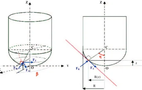
According to the tool geometry, the machi- ning surface breaks up into two distinct surfaces : the guiding surface S 1 which is the offset surface of the nominal surface, and

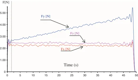
The cutting forces in machining are due to stresses in the primary shear plane, friction at the tool chip interface and friction at the flank face.. During Ti-5553 machining, this

In addition to the tool wear or cutting forces in titanium and aluminium layers, fractal dimension

The cutting edge wear process according to the cutting path in machined mate- rial shows three areas that characterize the behaviour of the tool edge recession, which are;

Using the best pressure and liquid/gas volume fraction inlet values determined previously, the main goal now is to analyze the influence of the tool channels geometry on the flow

& Straight penetration leads to more resultant cutting forces as compared to half revolution penetration and quarter revolution penetration strategies for all the three

On the other hand, increasing the tool helix angle decreases significantly the cutting friction but increases the machining damages in terms of fibers fluffing at the surface

The proposed modeling tool was developed to be used for PEM Fuel Cells charge and heat transfer modeling, it can provide several calculations and graphical results according to