Science Arts & Métiers (SAM)
is an open access repository that collects the work of Arts et Métiers Institute of
Technology researchers and makes it freely available over the web where possible.
This is an author-deposited version published in:
https://sam.ensam.eu
Handle ID: .
http://hdl.handle.net/10985/18996
To cite this version :
Bastien TOUBHANS, Guillaume FROMENTIN, Fabien VIPREY, Habib KARAOUNI, Théo
DORLIN - Machinability of inconel 718 during turning: Cutting force model considering tool wear,
influence on surface integrity Journal of Materials Processing Technology Vol. 285, p.116809
-2020
Any correspondence concerning this service should be sent to the repository
Administrator :
archiveouverte@ensam.eu
Machinability
of inconel 718 during turning: Cutting force model
considering
tool wear, influence on surface integrity
Bastien Toubhans
a,b,*
, Guillaume Fromentin
a, Fabien Viprey
a, Habib Karaouni
b, Théo Dorlin
baArts et Metiers Institute of Technology, LABOMAP, UBFC, HESAM Université, F-71250, Cluny, France bSafran S.A., Research & Technology Center, F-78772, Magny-les-Hameaux, France
A R T I C L E I N F O
Associate Editor: E Budak Keywords:
Cutting force model Tool wear Surface integrity Residual stresses Turning
A B S T R A C T
Machining accuracy can be compromised by elastic workpiece deformation and subsurface residual stress in-troduction during cutting. In order to anticipate the impact of cutting forces and surface integrity evolutions on finished surface and its geometrical errors, it is necessary to better understand the influence of cutting conditions and tool wear. In this study, machinability of Inconel 718 using a round carbide tool infinish turning conditions is assessed. Cutting forces evolution during tool life are analysed and accompanied by advanced investigations of cutting phenomena. An original mechanistic cutting force model is developed, identified and tested. It includes the effect of tool wear over time in its local formulation. This model allows predicting cutting forces evolution along tool pass for a wide range offinishing cutting conditions. Furthermore, a thorough analysis of residual stress profiles at different tool wear levels is led. It features quantitative results for fresh and worn tools. A study on the influence of cutting parameters and tool wear on residual stress profiles in the machining affected zone is highlighted.
1. Introduction
Accuracy is one of the major concerns when machining high-added value parts. Among the significant amount of possible sources of geo-metrical errors encountered in machining of thin parts, this study fo-cuses on two phenomena directly linked to the cutting action. Thefirst one is the workpiece elastic deformation under load during machining. As the workpiece is pushed away from the cutting tool, an undercut defect appears on thefinished part. The second one is the alteration of surface integrity during machining. Heterogeneous plastic deforma-tions, arising from multiple mechanisms during cutting, result in re-sidual stresses in a thin layer under the machined surface.Brinksmeier et al. (1982)find that these residual stresses can generate deformations
by disturbing the workpiece equilibrium. Although these two phe-nomena are often neglected when machining rigid parts, they may have a prominent role when dealing with low stiffness parts.Toubhans et al. (2019)quantify their influence. In the case of face turning on thin discs,
80 % of the total geometrical error is attributed to elastic part de-formation while 20 % is linked to machining induced residual stresses and stress rebalancing following material removal. These two phe-nomena depend on the material considered.
The material of this study is Inconel 718, a nickel-based alloy. It is
widespread in turbine engines for its remarkable mechanical and cor-rosion resistance properties at high service temperatures. Although the machinability of this material has been improved over the years, it remains a‘hard to cut’ material. Manufacturers are mainly struggling with low attainable cutting speeds and rapid tool wear. The presence of hard carbide particles in the microstructure, the low heat conductivity
and the Built Up Edge (BUE) phenomenon are evoked by Polvorosa
et al. (2017). These three characteristics, inherent to nickel alloys, are identified in the literature as responsible for rapid tool wear. When machining Inconel 718 with carbide tools in finishing conditions,
Devillez et al. (2007) establish that the main wear mechanisms are abrasion and adhesion. According to the same authors, on the one hand,
wear manifestations due to abrasion are mainly flank wear and
notching of the cutting edge. On the other hand, adhesion is responsible for coatingflaking and removal of material from the rake face.Arrazola et al. (2014)observe that tool wear and surface degradations appear faster above a certainflank wear around 0.15 mm. Tool life is often
determined by the amount offlank wear VB which can be measured
following theISO 3685 (1993). A value equal to 0.3 mm is currently considered in literature for carbidefinishing tools to deem a tool worn. In addition, cutting forces tend to rise with tool wear. When using round inserts forfinishing Inconel 718 in turning,Arrazola et al. (2014)
⁎Corresponding author at: Arts et Metiers Institute of Technology, LABOMAP, HESAM Université, F-71250, Cluny, France.
E-mail addresses:bastien.toubhans@ensam.eu,bastien.toubhans@free.fr(B. Toubhans),Guillaume.fromentin@ensam.eu(G. Fromentin), Fabien.viprey@ensam.eu(F. Viprey),Habib.karaouni@safrangroup.com(H. Karaouni),Theo.dorlin@safrangroup.com(T. Dorlin).
confirm that trend for the three cutting forces in the machine refer-ential. However, the passive cutting force, normal to the machined surface, appears to be much more sensitive to tool wear. Indeed, the passive cutting force level is multiplied by 5 during the tool life. The physical explanation given by Grzesik et al. (2018)is the ploughing effect favoured by tool wear.
Therefore, modelling cutting forces evolution in respect with cutting conditions and tool wear is a challenge. Numerous contributions are available in thefield of cutting force modelling. Different approaches emerged with time such as empirical, analytical and numerical as
Arrazola et al. (2013) relate. The present study focuses on the me-chanistic approach which is part of the empirical kind. In a meme-chanistic model, local forces are expressed as a linear function of the cut thick-ness. Among primary developments,Armarego and Cheng (1972)first
introduce the edge discretisation methodology in order to calculate global forces by summing local forces along the cutting edge.Armarego and Whitfield (1985) propose a two components local cutting force model describing what is known as the“cutting effect” and the “edge effect”. Kapoor et al. (1998)state the importance of modelling chip flow direction on accuracy. Indeed, consistent chip flow direction suggests a dependency between the cutting edge segments which is absent in Armarego’s formulation.Molinari and Moufki (2005)propose a mechanical cutting model based on the elementary chip equilibrium including a resulting force on its lateral sides, i.e. tangential to the cutting edge. Following this idea,Dorlin et al. (2016)andChérif et al. (2018), with a mechanistic approach, completed the original local force model used byArmarego and Whitfield (1985)by adding a third local force tangent to the cutting edge. It allows better prediction of cutting forces when machining with round insert or with the tool nose.
Several attempts have been made to take tool wear into account in cutting force models. A commonly found approach is to model the VB evolution during tool life and then incorporate it in a cutting force model. This method is used byZhu and Zhang (2019)with a time de-pendant wear model in high speed milling. Besides, an analytical model describing the evolution offlank wear is presented byDas et al. (2019).
Grzesik et al. (2018)develops a global empirical model considering the removed chip volume and the cutting speed in order to model theflank wear during tool life. Other approaches do not consider tool wear di-rectly but develop a mechanistic model with addition of a time de-pendent term. The instantaneous force is expressed as A + B(t) where, A is the cutting force level with no wear, and B(t) is a time dependant term representing the effect of wear.Lacalle et al. (2017)present a time dependent additional term considering cutting speed and feed rate in a global cutting force model without considering the nose radius effect. This last approach is considered in this study by means of a local cutting force model. This way, the nose radius effect, which is of prime im-portance when using round tools, is considered.
Concerning surface integrity, a wide consensus appears to describe the residual stress profiles in the machining affected layer of Inconel 718. Devillez et al. (2011)depict the typical profile as tensile on the
surface, decreasing toward a minimum compressive stress at shallow depth around couple hundreds of micrometres, and increasing back toward the bulk residual stress. Among the multiple parameters influ-encing the residual stress profile shape,Devillez et al. (2011) list the most influent as tool geometry, tool wear, cutting conditions and lu-brication.Sharman et al. (2006)describe that tool wear has the largest influence on surface integrity. Using a worn tool leads to higher tensile peak at the surface and deeper compressive stress. Sharman et al. (2006)argue that a worn cutting tool loses its ability to cleanly cut the material and tends to rub against the machined surface which leads to higher temperature and more plastic deformation. These observations are confirmed in a more recent study bySharman et al. (2015)using round tools. According toJavadi et al. (2019), there are no linear re-lationships between residual stress profiles and process parameters. Indeed, Thakur and Gangopadhyay (2016)show that it is widely ac-cepted in the community that the final residual stress profile is the
result of a competition between thermal and mechanical inputs during the cutting action. Thermal and mechanical loads respectively favour tensile and compressive stresses.
The literature related to the turning of Inconel 718 infinishing condition reveals that cutting forces and surface integrity are sig-nificantly influenced by cutting conditions and tool wear. In this study, the focus is set on developing a cutting force model taking tool wear into account during face turning. The second section presents the ex-perimental procedure. In the third section, a cutting force model is improved in order to predict the cutting forces when using a fresh tool. This model is generalised for different cutting speeds. In the fourth section, this model is complemented by an additional term to take tool wear into account. The fifth section focuses on the study of surface integrity depending on tool wear levels and cutting conditions. Finally, residual stress profiles analysis are compared to literature observations. 2. Study parameters and experimental setup
2.1. Material and cutting conditions
The material machined in this study in an Inconel 718 treated to 45 HRC. The cutting tool is a round carbide insert with a 4 mm nose radius. The cutting insert has a PVD micro grain (Ti,Al)N + TiN coating spe-cially designed for thefinishing of superalloys. When mounted in the tool holder, the rake, inclination and clearance angle are respectively 0°, 0° and 7°. Flood cooling conditions are applied using a water based emulsion with 5 % oil content.
The study focuses on face turning operation with constant cutting speed. Three cutting speeds are used, Vc∈ {35; 52.5; 70} m/min. Feed f
and depth of cut apare chosen in order to explore a range of maximum
cut thickness hmax∈ [0.05; 0.14] mm representative of finishing
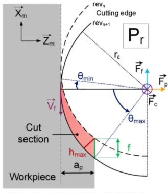
con-ditions. A description of the cut section geometry is given in Fig. 1
where the position of the cutting edge is given in the Prplane (cf.ISO 3002-1 (1982)) during one spindle revolution. The engaged portion of the cutting edge is bounded byθminandθmax, which depends on the
depth of cut ap, the feed f and the nose radius rε. The cut thickness h
varies along the cutting edge of a round insert and reaches its maximal value hmaxclose toθmax.
2.2. Experimental setup
The cutting tests are performed on a 3-axis CNC lathe. The global cutting forces are measured in-process in the machine coordinate system (MCS) with a piezoelectric dynamometer and a charge ampli-fier. In-situ measurements of flank wear is performed using a digital microscope to avoid disassembling the tool and the resulting re-positioning issues when using round inserts. VBmaxis measured (cf.ISO 3685 (1993)) and is called VB in this study. The goal is to monitor the cutting forces evolution during the tool life in order to predict it with a cutting force model presented in the next two sections.
3. Generalised cutting force model when using a fresh tool 3.1. Local forces model and edge discretisation methodology
This section focuses on the mechanistic approach to model cutting forces when using a fresh tool. This model is generalised for different cutting speeds. The experimental data are gathered through short dressing operations. Nine cutting tests with different engagements, summed up inTable 1, are performed for three different cutting speeds, giving 27 tests. The diameter range during these tests is [115; 84] mm. No significant wear is measured on the cutting inserts after these tests. Indeed, VB does not exceed 60μm which is consistent with flank wear values encountered during the running-in period. The cutting forces are averaged on three spindle turns during steady state. The measurements during the 27 cutting tests are available inTable 1. Considering the large nose radius and shallow depths of cut used, the edge orientation is such that Fpmodulus is important compared to Ffone. As expected, at
similar chip load, cutting forces decrease when the cutting speed in-creases. Therefore, the cutting speed is taken into account in the model. The local cutting forces model, displayed in Eq.(1), is calculated using the cutting edge discretisation methodology. The engaged cutting edge is discretised into N segments of equal lengths b as depicted in
Fig. 2. The local force model used in this study is based on Armarego’s
early work on cutting force modellingArmarego and Whitfield (1985). Armarego’s model considers two local force components acting on a cutting edge segment fvand fh, respectively axial and radial to the
cutting edge as depicted inFig. 2. Each component is expressed as a linear function of the local cut thickness h. An additional component, tangential to the cutting edge, is added. It ensures that the local forces on each segment contribute to the global chip flow direction. This tangential component fois proportional toηcf,i, the local gap between
the average chipflow direction θcfand the angular positionθiof the
considered segment as shown onFig. 2. The average chipflow direction θcfis computed using a geometric formulation shown in Eq.(1). This
formulation displays convincing correlation with experimental tests in Chérif’s study when the inclination angle is equal to zeroChérif et al. (2018). Finally, the effect of the cutting speed is added to the model by multiplying fvand fhby a dimensionless term Vc/Voraised to a certain
power (nvand nh) where Vo= 52.5 m/min. The cutting speed has a
limited influence of the average chip flow direction according to Chérif’s observation. As a consequence, the effect of Vcis not added to
fo. ⏟
∫
∫
⎜ ⎟ ⎜ ⎟ ⎧ ⎨ ⎪ ⎪ ⎪ ⎪ ⎪ ⎪ ⎩ ⎪ ⎪ ⎪ ⎪ ⎪ ⎪ = + ⎛ ⎝ ⎞ ⎠ = + ⎛ ⎝ ⎞ ⎠ = = − = k k k k k f b h V V f b h V V f b η h η θ θ θ h θ θ dθ h θ dθ ( . ). ( . ). . . . ( ). ( ) cv ev n ch eh n o v i i c o h i i c o o i cf i iChip flow effect cf i cf i cf θ θ θ θ , , , , , v h min max min max (1) Local forces are calculated on each segment according to the local force model. The global forces are then computed by projection and summation of the local forces in the MCS according to Eq.(2). Finally, the model coefficients are optimised by least square minimisation of the absolute error of the three global forces (Fc, Ffand Fp). The
Nelder-Mead simplex algorithm is used to optimise the solution. The data-set used to identify the model contains all measured data gathered from the 27 tests described above.
∑
∑
∑
⎧ ⎨ ⎪ ⎪ ⎪ ⎩ ⎪ ⎪ ⎪ = = − = + = = = F f F f θ f θ F f θ f θ . sin ( ) . cos ( ) . cos ( ) . sin ( ) c i N v i f i N h i i o i i p i N h i i o i i 1 , 1 , , 1 , , MCS MCS MCS | | | (2) Table 1Cutting conditions and mean cutting force measurements during short face turning tests. Vcis in m/min.
f ap hmax Fc_mean(N) Ff_mean(N) Fp_mean(N)
mm/rev mm mm Vc= 35 Vc= 52.5 Vc= 70 Vc= 35 Vc= 52.5 Vc= 70 Vc= 35 Vc= 52.5 Vc= 70 0.1 0.5 0.047 249 235 224 75 67 62 249 237 223 0.2 0.5 0.093 407 372 370 92 79 79 328 290 289 0.3 0.5 0.136 540 512 495 102 92 82 381 347 328 0.15 0.35 0.059 258 236 232 58 53 52 255 234 237 0.25 0.35 0.096 362 333 329 68 58 57 305 274 275 0.35 0.35 0.130 453 430 416 73 64 65 342 313 305 0.25 0.2 0.071 230 220 205 35 31 31 225 213 206 0.3 0.2 0.083 260 247 232 35 33 32 242 229 222 0.4 0.2 0.106 312 300 289 37 35 30 264 250 241
3.2. Cutting force modelling: results and discussions
The local forces model contains 7 unknown constants to identify, respectively kcv, kev, kch,keh, ko, nvand nh. The identified coefficients
are given inTable 2. The negative values of the exponents associated to the cutting speed terms are consistent with experimental observations. It can be noted that cutting speed has similar influence on both com-ponents fhand fv. Each of the 27 cutting tests gives 3 global forces data
samples. As a result, the Residual Degree Of Freedom (RDOF) for fv
model is equal to 24 and the one for fhand fois equal to 50. The RDOF is
calculated as the difference between the number of equations and the number of unknown parameters. For example, according to Eq. (2), there are 54 equations (27 Fp-samples and 27 Ff-samples) to compute
fhand foand 4 unknown constants giving a RDOF equal to 50. Cross
validations tests are performed by using only a portion of the experi-mental data-set to identify the model and the rest of the data-set for validation simulations. The identification results are similar when using half of the data-set, two thirds of the data-set and the entire data-set. Consequently, the well distributed data-set combined with the high model RDOF leads to a robust identification.
The errors between simulated and measured forces are displayed in
Fig. 3, with black points, for the three components Fc, Ffand Fp.Fig. 3is
a box plot where half of the data is contained in the boxes and the other half between the whiskers (dotted lines) outside the boxes. The whisker length is equal to 1.5 times the interquartile range or box length. Values outside the whiskers are called outliers and are symbolised by red crosses.
Although the maximum relative error on Ffseems important
com-pared to the other global forces, the levels of Ffare 6 times lower than
Fcand 5 times lower than Fp. Consequently, the absolute error on Ff
remains low. For the same reason, Ffis more sensitive to measurement
noise which explains why outliers are found only for Ff. This
discrepancy is due to the optimisation strategy which minimises the absolute error. Indeed, the global forces with the highest magnitudes are favoured by this optimisation strategy.
The presented three components model is compared to Armarego’s two component model. The prediction is unchanged for Fcas the fvlocal
force is the same for the two models and only appears in Fccalculation.
However, when including the third component foin the model, the
average relative error for Fpis divided by two and the average relative
error on Ffis slightly degraded (by 0.3 %). The relative error on Fpis
shown inFig. 4for the 9 cutting conditions used at Vc= 52.5 m/min
using both models. Both errors are evenly distributed around zero as dictated by the optimization strategy. However, three groups of red dots, corresponding to the two component model, are clearly identified. There is one group for each depth of cut used. Experimentally, changing the depth of cut modifies the length of the engaged cutting edge and hence the chipflow direction. In definitive,Fig. 4shows that the two component model lacks the description of the influence of chip flow direction on cutting forces. The same observation is made for the two other tested cutting speeds. Considering Eq.(1), the contribution of fo
component increases when the gap between the angular position of the considered segment and the average chipflow direction increases. This contributes to orientate Ffand Fpresultant alongθcfin the Prplane,
tangent to the rake face.
To conclude, a cutting force model is developed in order to give cutting forces when using a fresh cutting tool. It is valid on a certain range of cutting speeds and tool engagements representative of fin-ishing conditions in Inconel 718 using a carbide cutting tool. The ad-dition of a third component foin the local force model allows for better
prediction of the passive cutting force Fp, normal to the machined
surface, which is the principal responsible for elastic deformation of the workpiece under load. However, tool wear has the first role in the evolution of cutting forces during a normal tool life. The next section focuses on analysing cutting forces evolution with wear and improving the current model to take tool wear into account.
4. Cutting force model taking wear into account
In this section, experimental observations are presented concerning tool wear and cutting forces evolution during tool life. A specific paragraph deals with the built-up-edge effect on these two phenomena. Drawing conclusions from the experimental observations, a cutting force model taking tool wear into account is developed and tested Table 2
Identified coefficients of the local force model for fresh tool. Global forces Local forces RDOF Identified components
Fc fv(N) 24 kcv(N. mm−2) 2651 kev(N. mm−1) 57 nv(-) −0.136 Ff, Fp fh(N) 50 kch(N. mm−2) 1726 keh(N. mm−1) 104 nh(-) −0.144 fo(N) ko(N. mm−2. rad−1) 53807
Fig. 3. Relative and absolute errors between experimental and modelled cut-ting forces using the fresh tool cutcut-ting force model in Eq.(1).
Fig. 4. Influence of the third local force component fo on Fppassive force
4.1. Experimental observations
Cutting tests are performed to monitor tool wear and cutting forces evolution during tool life for 9 different cutting conditions. Three cut-ting speeds (35, 52.5, and 70 m/min) and 3 feed (0.1, 0.2, and 0.35 mm/rev) are explored. The depth of cut is kept constant at 0.5 mm. Then, three levels of hmax= {0.047; 0.093; 0.16} mm are explored. A
fresh cutting tool is used for each test. The tests consist of long similar
facing operations repeated until the tool is deemed worn
(VB > 0.3 mm). The diameter range during these tests is [150; 45] mm.
4.1.1. Tool wear mechanisms and manifestations
Experimental observations agree with the literature, adhesion and abrasion are the main tool wear mechanisms. Most of tool wear man-ifestations appear on the flank face and consist of tool abrasion, smeared material, notching and collapsing of the cutting edge as shown onFig. 5. Flank wear tends to become uneven when cutting speed and feed increases (Fig. 5.b). Indeed, some wear facies display more wear in the area where the cut thickness is important. Small notches appear on the cutting edge at elevated speeds (Fig. 5.b). It is thought to be tracks left when the cutting edge encounters hard carbides present in the material. Cutting edge collapse (Fig. 5.c) appears at highest cutting speeds and low feed.
As the metal is being cut, some material stagnates in front of the cutting edge. It is commonly called a Built-Up Edge (BUE) and can be seen in Fig. 5.a above the red line materialising the original cutting edge. Some of it accumulates on the tool rake face forming a Built-Up Layer (BUL). Meanwhile, some of it is evacuated between the cutting tool and the machined surface. This material ends up smeared on the machined surface and the tool flank face as one can observe on the Scanning Electron Microscope (SEM) image onFig. 6. Built-Up Edge is observed for every tested cutting condition. To sum up, increasing cutting speed and feed tends to favourflank wear unevenness and more dramatic changes of the cutting edge geometry. These changes in cut-ting edge geometry may cause important variations of cutcut-ting forces as analysed in the next paragraph.
4.1.2. Cutting forces evolution during tool life
OnFig. 7, cutting forces are represented as a function of machining time during the test at the following cutting conditions, Vc=70 m/min,
f =0.1 mm/rev and ap=0.5 mm. The discontinuities on the curves are
the transitional regimes between each pass which have been cut out for legibility. This particular test took 5 passes to reach the criticalflank wear level VB > 0.3 mm. A typical cutting force evolution is observed with a short running-in period followed by a controlled wear region and finally by the tool end of life. Cutting forces tend to increase with tool wear. However, the passive cutting force Fp, normal to the machined
surface, is more sensitive to it than Fcand Ff. It is consistent with
ob-servations made byArrazola et al. (2014)in comparable conditions. During a normal tool life, Fpis multiplied by 3–7 while Fcand Ffare
multiplied by 2–4 depending on the cutting conditions.
Tool wear is known to be a phenomenon with poor repeatability. To ensure that cutting forces can be modelled, reproducibility tests are performed for certain cutting conditions. OnFig. 8, passive force Fp
evolution is illustrated during three repetitions of the same wear test. It appears that in the studied case, the running-in and controlled wear regions display repeatability. However, the inflection point towards the tool end of life, materialised by dashed lines, is quite variable. There are several factors able to disturb a stable wear evolution. Indeed, when the tool is wearing, the cutting edge integrity is compromised and prone to catastrophic failures, such as collapsing of the cutting edge, which may cause the inflexion point occurrence to vary. Same remark applies to notching of the cutting edge which creates a starting point for cata-strophic failure. Moreover, notching randomly occurs at any time during tool life. Furthermore, entering and exiting the material are critical times for wear evolution as transitional regime may imply Fig. 5. Flank wear manifestations depending on cutting conditions.
Fig. 6. SEM image of a tool with wear manifestations and BUE - Vc= 35 m/
min, f = 0.1 mm/rev, ap= 0.5 mm.
Fig. 7. Typical cutting forces evolution during tool life - Vc= 70 m/min, f =
sudden changes in loadings and provoke modifications of the cutting edge geometry.
Tool wear tends to favour BUE formation. Indeed, as the cutting edge becomes dull, more material seems to stagnate in its vicinity. At low cutting speeds, BUE has a significant effect on cutting forces evo-lution. This phenomenon is detailed in the next paragraph.
4.1.3. Built-Up Edge effect on cutting forces evolution
When performing wear tests at the lowest cutting speed 35 m/min, perturbations of the cutting forces evolution occur (Fig. 9). Instead of having continuous evolution as observed in Fig. 7, long period oscil-lations on all cutting forces, discontinuity between passes and peaks when engaging and disengaging the tool appear. The slight dis-continuity between thefirst passes observed onFig. 9may be explained by the grain size gradient along the workpiece radius. Indeed, the average grain size is equal to 12μm close to the outer diameter and 50μm close to the inner diameter. It results in a moderate hardness gradient along the radius, 45 HRC forfine grain structure and 43 HRC for coarser grain structure. Additionally, as stated by Olovsjö et al. (2010), the adhesion related phenomenon are more pronounced in coarser grain structure. It could be another factor explaining the rise of cutting forces observed in the coarser grain structure at the end of the first passes onFig. 9.
During the long period oscillations, cutting forces drop significantly, up to 45 % for Fp, compared to their expected levels. Several possible
causes, such as heterogeneous hardness along the radius, poor chip evacuation or temporary loss of lubrication due to chip accumulation in the cutting zone, are discarded due to the magnitude of the oscillations. Process damping might have occurred at lower speed considering the ploughing effect due to BUE formation and the extent of flank wear. However, the low frequency oscillations, under 0.1 Hz, cannot be linked to process damping as it is far from the process frequencies.
These phenomena, which manifest above certain wear level, are thought to be adhesion related. Indeed, at lower cutting speeds, the BUE may become stable and act as a substitute cutting edge. As illu-strated onFig. 10, in presence of a BUE, it is supposed that the rake angle becomes more positive and the contact between theflank face and the machined surface is interrupted. The consequence of these two factors is a cutting forces drop. Indeed, the rubbing of the toolflank face on the machined surface is a major contributor to global cutting forces. The oscillations would be resulting from the alternation of evacuation and reformation of the BUE.
This assumption is supported by further analysis. This test is re-peated and the machined surface is scanned with a laser profilometre along the workpiece radius after a pass during which perturbations occurred. The passive cutting force during this pass is superimposed with the machined surface topography onFig. 11. Reliefs are observed on the machined surface. Valleys, 30μm deep on average, are measured and correlated with forces drops. These observations checks with the BUE hypothesis as BUE acts as a substitute cutting edge made of stag-nating material which slightly increases the depth of cut.
From the above observations, it is recommended to avoid cutting conditions where BUE is stable as it will greatly degrade accuracy and surface roughness. Thefirst choice is to increase the cutting speed. During the performed tests, increasing Vcfrom 35 to 52.5 m/min made
these phenomena disappear as BUE may have become unstable. Considering the significant increase of all cutting forces during a normal tool life, tool wear influence is added to the cutting force model in the next section.
4.2. Cutting force model development 4.2.1. Formulation of the model
In section3, a mechanistic model designed to give cutting forces when using a fresh tool is presented. Previous observations made it clear that cutting forces increase during tool life. Hence, in this section, the previous model is complemented by an additional term to take wear into consideration. Additionally, only the running-in and controlled wear periods are modelled as the inflexion point toward the tool end of life is unpredictable.
Fig. 8. Evolution of Fppassive force during three repetitions - Vc= 70 m/min, f
= 0.1 mm/rev and ap= 0.5 mm.
Fig. 9. Unstable cutting forces evolution during wear test - Vc= 35 m/min, f =
0.1 mm/rev and ap= 0.5 mm.
Fig. 10. Effect of built-up edge formation on cutting geometry and tribology.
Fig. 11. Correlation between cutting forces drops and negative reliefs on ma-chined surface.
Toolflank wear VB is measured during the tests but is not used to model the effect of wear on cutting forces evolution. Indeed, measuring flank wear implies a stoppage of the cutting process. VB measurements are performed after each pass. As a consequence, few measurements are done during the tests to ensure realistic test durations and to limit the number of tool engagement cycles which favour quick wear. In addi-tion, wear manifestations such as smearing on theflank face, notches or wear unevenness (seeFig. 5) make it more complicated to accurately measure VB. Instead of using a parameter directly linked to tool wear, such as VB, the cutting force evolution is modelled in relation to a process parameter which can be continuously measured during the cutting tests.
Parameters such as the cumulated uncut chip length Lmand
re-moved volume Vmor cumulated machining time tmare considered. Lm
is the real distance travelled by the generative point of the tool (i.e. an Archimedes’ spiral during facing). Vm is Lm multiplied by the
un-deformed chip cross sectional area. The idea is to represent the actual amount of work done by the cutting edge during its life. Exploratory developments are made by adding a power function term of Lmor Vmto
the fresh tool model. However, Lmand Vmare global quantities and
there is no bijection between them and the actual cut area represented by f and ap. Indeed, Lmis independent of apand Vmis independent of f
(cf. Appendix A for supplementary equations). Consequently, these models are discarded.
The most advanced model is presented in Eq.(3). An additional term is added to fhand fvformula. So the global forces are expressed as
A + B(t) where A is the cutting force level when the tool is fresh and B (t) represents the force increase due to wear over time. The fo
compo-nent is untouched as chip flow direction is unaffected by tool wear according to experimental observations in similar conditions (Chérif et al. (2018)). Considering constant lubrication conditions, cutting speed is the most influent process parameter on tool life followed by feed and depth of cut. In this model, the feed and depth of cut effects are encapsulated in the local cut thickness hiwhich represents the chip
load. Finally, the additional term takes the form of a power function of machining time, cutting speed and local cut thickness with 8 new coefficients to identify, respectively kwv, nhv, ntv, nvv, kwh, nhh, nthand
nvh. It can be noted that fvand fhlocal formulations now contain two
terms depending on Vc/Vo with different power exponents. Indeed,
cutting speed has significant influence on both cutting forces initial level and evolution over time.
⏟ ⏟ ⏟ ⏟ ⎜ ⎟ ⎜ ⎟ ⎜ ⎟ ⎜ ⎟ ⎧ ⎨ ⎪ ⎪ ⎪ ⎪ ⎪ ⎩ ⎪ ⎪ ⎪ ⎪ ⎪ = ⎛ ⎝ ⎜ ⎜ ⎜ + ⎛ ⎝ ⎞ ⎠ + ⎛ ⎝ ⎞ ⎠ ⎞ ⎠ ⎟ ⎟ ⎟ = ⎛ ⎝ ⎜ ⎜ ⎜ + ⎛ ⎝ ⎞ ⎠ + ⎛ ⎝ ⎞ ⎠ ⎞ ⎠ ⎟ ⎟ ⎟ = k k f b k h k V V h t V V f b k h k V V h t V V f b k η h ( . ). . . . ( . ). . . . . . . wv n n n wh n n n v i cv i ev c o n A fresh tool i c o B t wear effect h i ch i eh c o n A fresh tool i c o B t wear effect o i o cf i i , ( ) ( ) ( ) , ( ) ( ) ( ) , , hv tv vv hh th vh v h (3) 4.2.2. Identification of the model and discussions
The seven coefficients which are identified in section3.2for the fresh tool model are kept in the new model. The same edge dis-cretisation is used to identify the eight new coefficients. To do so, ex-perimental data are gathered by discretising the cutting forces evolu-tion curves over machining time. The test at Vc= 35 m/min and f =
0.1 mm/rev is not used for the identification as the cutting force evo-lution is highly disturbed by the BUE related phenomenon presented in section4.1.3.
The identification results are presented inTable 3. The simulated cutting force evolutions are plotted inFig. 12against the experimental samples for each test. An average of 20 samples per test and per cutting force (Fc, Ff and Fp) is selected. As a result, the model is highly
overdetermined as evidenced by the residual degree of freedom (cf.
Table 3). These samples are represented by discrete markers inFig. 12. The sampling is denser in the running-in region as the cutting forces evolution is less linear than during the controlled wear region. As it is shown inFig. 12, the model is able to predict the evolution of the three cutting force components in the machine referential. In the next para-graphs, this model is evaluated on its ability to predict the cutting force evolution, especially the passive cutting force which is the most sensi-tive to tool wear.
The maximum and median values of absolute and relative errors are given in Fig. 13. While the average error values are quite low, the discrepancy between the maximum and average values and the pre-sence of numerous outliers are questionable.
In order to better visualise the results, a box plot is displayed in
Fig. 14to evaluate the prediction of the passive cutting force Fp. The
black dots represent the actual distribution of relative error between the experimental and simulated forces for each test. Additional values such as the average error, median, 25th and 75th percentiles are displayed on each box plot.
InFig. 14, the median value indicates the ability of the model to simulate a correct force evolution over time due to tool wear. If the median is close to zero, the slope is correct (Fig. 12(b,f)). If the median is over or under zero, the simulated slope respectively overestimate or underestimate the slope as inFig. 12(e,h). Overall, the model is able to simulate the passive cutting force evolution during the running-in and controlled wear region within 10 % of relative error in the tested range of cutting conditions.
During cutting tests‘a’ and ‘b’, the simulated slopes are correct but the error values are scattered and present outlying values. These iso-lated errors have two possible origins. The first is linked to dis-continuity between passes that appear during the tests at lower cutting speeds, where built-up edge disturbs the cutting forces evolution as mentioned in Section4.1.3. It means that the samples are on either side of the simulated evolution curves as shown inFig. 12a after 15 min of machining. It is evidenced by the negative and positive isolated errors on the‘a’ distribution inFig. 14. The second is linked to random effects
that manifest as slope modification, named bends, in the experimental cutting force evolution curves. These bends may randomly appear at higher speeds and disturb the nearly linear evolution of cutting forces during the controlled wear period. They are thought to be due to modification of the cutting edge geometry when notches or cutting edge collapse occur. Such a bend appears at the beginning of the second pass during the test at Vc= 52.5 m/min and f = 0.35 mm/rev (Fig. 12e)
causing the simulated slope to be wrong from the beginning. As it can be seen inFig. 12(e,g,h), higher cutting speeds and feed are impractical as the controlled wear region duration does not exceed two minutes.
In the studied case, transient regimes do not have a significant effect on cutting force evolutions during the running-in and controlled wear regions. Indeed, no significant cutting force discontinuity is observed between passes (seeFigs. 7 and 8). For this reason, to a certain extent, the model is valid for different workpiece diameters which would have more or less enter/exit tool periods.
To conclude this section, a local force model able to give the Table 3
Identified coefficients of the local force model taking wear into account. Global forces Local forces RDOF Identified coefficients
Fc fv(N) 155 kwv(-) 131 nhv(-) 0.58 ntv(-) 0.56 nvv(-) 1.32 Ff, Fp fh(N) 314 kwh(-) 147 nhh(-) 0.46 nth(-) 0.71 nvh(-) 2.19
evolution of cutting forces relative to tool wear during most of the tool life is developed. This model is valid on the tested range offinishing conditions during the running-in and controlled wear regions. However, variability in bulk material characteristics and unpredictable catastrophic wear manifestations are significant causes of gaps between experiment and model. In addition to its influence on cutting forces evolution, cutting tool wear has a significant impact on surface integrity which will be the next section focus.
5. Surface integrity analysis 5.1. Experimental approach
In this section, residual stress profiles of the machined surface are presented for various cutting conditions and tool wear levels. The specimens are 35 mm thick cylinders, considered as rigid bodies, to ensure no deformation due to machining induced stress or residual
stresses rebalancing following material removal. Face-turning
operations are performed until the tool is deemed worn. The diameter range during these tests is [155; 30] mm. Flat steps are machined on the specimen face in order to preserve the machined surface integrity at strategic time as it is depicted on the top view inTable 5. Five cutting conditions are tested based on experimental observations made in Section4.1. Cutting conditions as well as wear levels and machining times (tm) associated to each step are listed inTable 4. Compared with
the classic cutting force evolution during tool life displayed inFig. 7, thefirst step matches the end of the running-in period. The last step represents the tool end of life. The intermediate step corresponds to the end of the controlled wear region before the inflexion point. Stress measurements in the circumferential and radial directions are per-formed on the machinedflat steps by an X-Ray diffraction apparatus (DRX). The axial stresses are not studied. The uncertainty of residual stresses measurements is estimated at ± 40 MPa based on repeatability tests on a standard specimen. Profiles are built by incrementally eroding the machined surface to allow for stress measurements at dif-ferent depths using electropolishing. Generating a flat hole bottom using this technique is difficult, especially for deep holes. The Fig. 12. Experimental vs modelled cutting forces during running-in and controlled tool wear region.
Fig. 13. Relative and absolute errors between experimental and modelled cutting forces using the cutting force model in Eq.(3).
Table 4
Machining time andflank wear levels associated to every step.
Vc(m/min) 35 52.5 52.5 52.5 70
f (mm/rev) 0.1 0.1 0.2 0.35 0.1
ap(mm) 0.5
Step 1 tm= 5.2 min tm= 1.36 min tm= 0.68 min tm= 0.24 min tm= 0.44 min
VB = 0.13 mm VB = 0.1 mm VB = 0.09 mm VB = 0.07 mm VB = 0.1 mm
Step 2 tm= 7.03 min tm= 3.86 min
VB = 0.16 mm VB = 0.12 mm
Step 3 tm= 47.7 min tm= 20.2 min tm= 11.5 min tm= 6.9 min tm= 8.83 min
VB = 0.3 mm VB = 0.3 mm VB = 0.3 mm VB = 0.3 mm VB = 0.29 mm
Table 5
uncertainty of depth measurements is evaluated at 10 % of the target depth by laser measurements.
5.2. Effect of tool wear on residual stress
The residual stress profiles matches the literature observations stated in the introductionSharman et al. (2015). The comparison be-tween the profiles when using a fresh tool and a worn tool demonstrates a strong trend as shown in Fig. 15. This graph represents the cir-cumferential residual stresses for 3 wear levels during the test at
Vc= 52.5 m/min and f = 0.2 mm/rev. Machining with a worn tool
increases the tensile stress on the surface and the compressive stress at the compressive peak. Moreover, the affected depth increases by a factor 5 and the compressive peak is deeper, for every tested cutting conditions and in both measured directions. While the difference be-tween a fresh tool (light green circle curve) and a worn tool (red square curve) is remarkable, the intermediate profile (dark green diamond curve) shows moderate difference relative to the fresh tool profile. This observation is comparable to the cutting forces evolution during the test shown in the top right corner ofFig. 15. The steep increase in cutting forces occurs when the tool reaches a certain dullness which corre-sponds to aflank wear level VB between 0.15 and 0.2 mm. After this inflexion point, the cutting edge becomes extremely dull as evidenced by the rightmostflank wear picture inFig. 15.
The worn cutting edge geometry is the major factor influencing stress profile shape. However, it seems that stress profiles are moder-ately impacted by tool wear until VB reaches the tipping point between 0.15 and 0.2 mm. The effect of cutting conditions combined with tool wear is analysed in the next paragraph.
5.3. Effect of cutting conditions on residual stress
The effect of cutting conditions and tool wear on residual stress profiles shape is shown inTable 5. Global trends are described in re-sponse to an increase in feed or cutting speed. The latter are given for both tool states: a run-in tool and a worn tool in both measurement directions. Indicators such as the magnitude of the tensile and com-pressive peaks, depth of the comcom-pressive peak and affected depth are considered. The trends are symbolised by blue arrows modifying the typical residual stress profile (solid red line). Due to the discrete nature of the residual stresses measurements and the depth limitations, it may be risky to infer trends. When no trend can be extracted from the data, an orange cross is placed instead of an arrow. For example, the depth of the machining affected zone may be hazardous to analyse for the fol-lowing reasons. When the stress does not reach equilibrium at the deepest measured point or if the measurement spacing is too large. However, the difference of affected depth when using a run-in tool and a worn tool is noticeable and respectively evaluated at 0.1 mm and
0.5 mm on average.
Residual stress profiles are displayed inFig. 16to completeTable 5. The subfigureFig. 16a and c depict the effect of cutting speed on re-sidual stresses in the circumferential direction in function of tool wear. TheFig. 16b and d show the effect of feed on residual stresses in the
radial direction. Indeed, residual stresses appear to be more sensitive to cutting speed or feed evolutions in their respective directions, i.e. cir-cumferential for Vcand radial for f.
As illustrated byFig. 16 a, an increase in cutting speed tends to lower the surface tensile stresses when using a run-in tool. This ob-servation is consistent with the literature when using round carbide tools in wet or dryfinishing conditions and for moderate cutting speeds under 80 m/min Devillez et al. (2007); Pawade et al. (2007) and
Sharman et al. (2006). In addition, when using a run-in tool, the pro-files shapes are comparable while Vc is greater than 52.5 m/min as
shown in Fig. 16 a. However, the profile at Vc = 35 m/min is
in-comparable as it presents a deeper affected zone. The ploughing effect resulting from BUE formation could explain this discrepancy as the material stagnating at the cutting edge tends to create more compres-sive stress ahead of the tool.
When using a run-in tool at Vc= 52.5 m/min, increasing the feed
tends to favour tensile stresses on the surface and to reduce the mag-nitude and depth of the compressive peak in the radial direction (see
Fig. 16 b). Same trends are observed by Sharman et al. (2006) in comparable cutting conditions except for the compression peak depth which increases with feed rate.Sharman et al. (2015)discuss that the increase in surface tensile stress is linked to an increase in cutting force and possibly heat generation due to the higher chip volume being re-moved.
Moreover, compressive surface residual stresses are obtained when using a fresh tool at high cutting speeds and low feed namely Vc =
{52.5; 70} m/min and f = 0.1 mm/rev. This state of stress is desirable to enhance fatigue strength. However, machining with these conditions when the tool is worn leads to high surface tension as shown inFig. 16c and d which is detrimental for fatigue behavior.
Some stress profiles display brutal changes in the first microns under the machined surface as shown inFig. 16c (blue curve) and
Fig. 16d (light green curve). These rapid evolutions are consistent with a high heatflux at the surface which can induce metallurgical mod-ifications at the vicinity of the machined surface.
To summarize, tool wear has a moderate impact on residual stresses profiles shape while the flank wear VB is lower than a critical value between 0.15 mm and 0.2 mm. Above this critical value, the profiles are dramatically changed displaying high surface tension and deep affected zones. Using high cutting speeds and low feed tend to favor compressive stress at the surface and shallow affected depth in the controlled wear region.
6. Conclusions
This study presents a new local formulation of cutting force model considering the effect of tool wear over time. In addition, the effect of tool wear on surface integrity is analysed. The key conclusions are:
•
Including a third component, relative to chipflow direction, in the local force model, allows better prediction of cutting forces when using round inserts. In particular, the relative error on the passive cutting force is divided by 2.•
The new local formulation accurately predicts the cutting forces evolution over a wide range of finishing parameters during the running-in and controlled wear periods. Variability of tool wear evolution is still an obstacle to develop fully robust models.•
Tool wear has a critical impact on cutting forces and surfacein-tegrity. In this study, the passive cutting force is multiplied by up to 7 over tool life. Concerning surface integrity, the affected depth is multiplied by 5 and reaches 0.5 mm when machining with a worn Fig. 15. Circumferential residual stress profile at different wear levels and
tool. The residual stresses profiles obtained with worn tools display a highly compressive state in subsurface combined with elevated tensile stress close to the machined surface.
•
Wear has limited influence on residual stresses profiles shape while theflank wear VB remains under a critical value between 0.15 mm and 0.2 mm.This study brings physical analysis and model necessary to deal with the challenge of machining workpiece with low stiffness. Moreover, the presented cutting force model offers promising foundation for the de-velopment of strategies to compensate workpiece deflexion. Indeed, the update of tool trajectories to accommodate with workpiece elastic de-formation is a meaningful perspective in order to improve geometrical quality of thin machined parts. Furthermore, in order to anticipate distortions linked to machining induced residual stresses, a major helpful step would be to establish further model of residual stress based on mechanistic approach as developed bySu et al. (2013).
CRediT authorship contribution statement
Bastien Toubhans: Conceptualization, Methodology, Writing
-review & editing. Guillaume Fromentin: Conceptualization,
Methodology, Supervision, Validation. Fabien Viprey:
Conceptualization, Methodology, Supervision, Validation. Habib
Karaouni: Validation, Resources. Théo Dorlin: Validation, Resources.
Declaration of Competing Interest
The authors declare that they have no known competingfinancial interests or personal relationships that could have appeared to influ-ence the work reported in this paper.
Acknowledgements
This research did not receive any specific grant from funding agencies in the public, commercial, or not-for-profit sectors. The au-thors wish to thank T. Bergey from ArianeGroup for sharing his ex-pertise on X-ray diffraction measurements.
Appendix A. Supplementary equations
(Dmin; Dmax) = Minimum and maximum machined diameters
Minimum angular position on the engaged cutting edge
=
( )
−θ arcsin f
rε
min 2
Maximum angular position on the engaged cutting edge
=
(
−)
θ arcos 1 ap
rε
max
Maximum cut thickness
=r− r−a + r − r−a −f
hmax ε (ε p)² ( ε2 (ε p)2 )²
Angular position of hmax = −
−
(
)
θ arcos rε ap
rε hmax
hmax
Local cut thickness
⎧ ⎨ ⎩ > = − < = + − − − if θ h r if θ h r f θ r f cos θ θ , θ , . sin( ) . ( ) i i ε rε ap θi i i ε i ε i hmax cos( ) hmax 2 2 2 Machined length Lm= π. (D −D ) f max min 4 . 2 2 Machined volume V =L . .f a = . (D −D ) m m p π ap max min . 4 2 2
References
Armarego, E.J.A., Cheng, C.Y., 1972. Drilling withflat rake face and conventional twist drills—I. Theoretical investigation. Int. J. Mach. Tool Des. Res. 12, 17–35.
Armarego, E.J.A., Whitfield, R.C., 1985. Computer based modelling of popular machining operations for force and power prediction. CIRP Ann. 34, 65–69.
Arrazola, P.J., Özel, T., Umbrello, D., Davies, M., Jawahir, I.S., 2013. Recent advances in modelling of metal machining processes. CIRP Ann. 62, 695–718.
Arrazola, P.J., Garay, A., Fernandez, E., Ostolaza, K., 2014. Correlation between tool flank wear, force signals and surface integrity when turning bars of Inconel 718 in finishing conditions. Int. J. Mach. Mach. Mater. 7 (15), 84–100.
Brinksmeier, E., Cammett, J.T., König, W., Leskovar, P., Peters, J., Tönshoff, H.K., 1982. Residual stresses— measurement and causes in machining processes. CIRP Ann. 31, 491–510.
Chérif, I., Dorlin, T., Marcon, B., Fromentin, G., Karaouni, H., 2018. Phenomenological study of chipflow/formation and unified cutting force modelling during Ti6Al4V alloy turning operations. Procedia CIRP 77, 351–354.
Das, R., Joshi, S.S., Barshilia, H.C., 2019. Analytical model of progression offlank wear land width in drilling. J. Tribol. 141.
Devillez, A., Schneider, F., Dominiak, S., Dudzinski, D., Larrouquere, D., 2007. Cutting forces and wear in dry machining of Inconel 718 with coated carbide tools. Wear 262, 931–942.
Devillez, A., Le Coz, G., Dominiak, S., Dudzinski, D., 2011. Dry machining of Inconel 718, workpiece surface integrity. J. Mater. Process. Technol. 211, 1590–1598.
Dorlin, T., Fromentin, G., Costes, J.-P., 2016. Generalised cutting force model including contact radius effect for turning operations on Ti6Al4V titanium alloy. Int. J. Adv. Manuf. Technol. 86, 3297–3313.
Grzesik, W., Niesłony, P., Habrat, W., Sieniawski, J., Laskowski, P., 2018. Investigation of tool wear in the turning of Inconel 718 superalloy in terms of process performance and productivity enhancement. Tribol. Int. 118, 337–346.
ISO 3002-1, 1982. Basic Quantities in Cutting and Grinding— Part 1: Geometry of the Active Part of Cutting Tools— General Terms, Reference Systems, Tool and Working Angles, Chip Breakers.
ISO 3685:1993, 1993. Tool-life Testing With Single-point Turning Tools.
Javadi, H., Jomaa, W., Songmene, V., Brochu, M., Bocher, P., 2019. Inconel 718 Superalloy Controlled Surface Integrity for Fatigue Applications Produced by Precision Turning. Int. J. Precis. Eng. Manuf. 1–14.
Kapoor, S.G., DeVor, R.E., Zhu, R., Gajjela, R., Parakkal, G., Smithey, D., 1998. Development of mechanistic models for the prediction of machining performance: model building methodology. Mach. Sci. Technol. 2, 213–238.
de Lacalle, L.N.L., Pelayo, G.U., Fernández-Valdivielso, A., Alvarez, A., González, H., 2017. Wear-dependent specific coefficients in a mechanistic model for turning of nickel-based superalloy with ceramic tools. Open Eng. 7, 175–184.
Molinari, A., Moufki, A., 2005. A new thermomechanical model of cutting applied to turning operations. Part I. Theory. Int. J. Mach. Tools Manuf. 45, 166–180.
Olovsjö, S., Wretland, A., Sjöberg, G., 2010. The effect of grain size and hardness of wrought Alloy 718 on the wear of cemented carbide tools. Wear 268, 1045–1052.
Pawade, R.S., Joshi, S.S., Brahmankar, P.K., Rahman, M., 2007. An investigation of cutting forces and surface damage in high-speed turning of Inconel 718. J. Mater. Process. Technol. 192–193, 139–146.
Polvorosa, R., Suárez, A., de Lacalle, L.N.L., Cerrillo, I., Wretland, A., Veiga, F., 2017. Tool wear on nickel alloys with different coolant pressures: Comparison of Alloy 718 and Waspaloy. J. Manuf. Process. 26, 44–56.
Sharman, A.R.C., Hughes, J.I., Ridgway, K., 2006. An analysis of the residual stresses generated in Inconel 718TMwhen turning. J. Mater. Process. Technol. 173, 359–367. Sharman, A.R.C., Hughes, J.I., Ridgway, K., 2015. The effect of tool nose radius on surface
integrity and residual stresses when turning Inconel 718TM. J. Mater. Process. Technol. 216, 123–132.
Su, J.-C., Young, K.A., Ma, K., Srivatsa, S., Morehouse, J.B., Liang, S.Y., 2013. Modeling of residual stresses in milling. Int. J. Adv. Manuf. Technol. 65, 717–733.
Thakur, A., Gangopadhyay, S., 2016. State-of-the-art in surface integrity in machining of nickel-based super alloys. Int. J. Mach. Tools Manuf. 100, 25–54.
Toubhans, B., Viprey, F., Fromentin, G., Karaouni, H., 2019. Prediction of form error during face turning onflexible Inconel 718 workpiece. Procedia CIRP 82, 290–295.
Zhu, K., Zhang, Y., 2019. A generic tool wear model and its application to force modeling and wear monitoring in high speed milling. Mech. Syst. Signal Process. 115, 147–161.