Case studies of incorporation of prior information in electrical resistivity tomography: comparison of different approaches

Case studies of incorporation of prior information in electrical resistivity tomography: comparison of different approaches

Caterina David1*, Hermans Thomas2* andNguyen Frédéric3 1

F.R.I.A-FNRS, ArGEnCo – GEO³, Applied Geophysics, Liege University, Chemin des Chevreuils 1, B-4000 Liege, Belgium

2

Research fellow F.R.S-FNRS, ArGEnCo – GEO³, Applied Geophysics, Liege University, Chemin des Chevreuils 1, B-4000 Liege, Belgium

3

ArGEnCo – GEO³, Applied Geophysics, Liege University, Chemin des Chevreuils 1, B-4000 Liege, Belgium

Received October 2012, revision accepted November 2013 *The two first authors contributed equally to the publication

Corresponding author: Hermans Thomas, Chemin des Chevreuils 1, 4000 Liege, Belgium, thomas.hermans@ulg.ac.be

The final version of this paper is published in Near Surface Geophysics, a publication of the European Association of Geoscientists & Engineers and can be accessed at http://nsg.eage.org/publication/publicationdetails/?publication=76904

Please cite as:

Caterina, D., Hermans, T., and Nguyen F. 2014. Case studies of incorporation of prior information in electrical resistivity tomography: comparison of different approaches. Near Surface Geophysics, 12(4), 451-465. doi:10.3997/1873-0604.2013070

ABSTRACT

Many geophysical inverse problems are ill-posed and their solution non-unique. It is thus important to reduce the amount of mathematical solutions to more geologically plausible models by regularizing the inverse problem and incorporating all available prior information in the inversion process. We compare three different ways to incorporate prior information for electrical resistivity tomography (ERT): using a simple reference model or adding structural constraints to Occam's inversion and using geostatistical constraints. We made the comparison on four real cases representing different field applications in terms of scales of investigation and level of heterogeneities. In those cases, when electromagnetic logging data are available in boreholes to control the solution, it appears that incorporating prior information clearly improves the correspondence with logging data compared to the standard smoothness constraint. However, the way to incorporate it may have a major impact on the solution. A reference model can often be used to constrain the inversion; however, it can lead to misinterpretation if its weight is too strong or the resistivity values inappropriate. When the computation of the vertical and/or horizontal correlation length is possible, the geostatistical inversion gives reliable results everywhere in the section. However, adding geostatistical constraints can be difficult when there is not enough data to compute correlation lengths. When a known limit between two layers exists, the use of structural constraint seems to be more indicated particularly when the limit is located in zones of low sensitivity for ERT. This work should help interpreters to include their prior information directly into the inversion process through an appropriate way.

INTRODUCTION

Most geophysical inverse problems are ill-posed due to the non-existence, non-uniqueness or instability of the solution. The non-linearity of the forward problem and the limited number of data against the number of parameters are causes for the non-uniqueness of the solution (see e.g., Menke 1984 or Aster et al. 2005). A common way to solve inverse problems is to add regularization to a least-squares problem (e.g., Tikhonov and Arsenin 1977).

Smoothness constrained regularization (Constable et al. 1987) is a standard technique to regularize inverse problems in applied geophysics, especially in electric and electromagnetic problems (deGroot-Hedlin and Constable 1990). However, in many cases, such constraint is not consistent with the geology (e.g., Blaschek et al. 2008; Robert et al. 2011; Hermans et al. 2012b). For example, when the subsurface resistivities do not vary in a smooth manner, one may use other regularization techniques such as the L1 norm model constraint (Farquharson and Oldenburg 1998; Loke et al. 2003). If prior knowledge allows, one should reduce the amount of mathematical solutions to more geologically plausible models by incorporating all available prior information in the inversion process (e.g., Blakely 1995, chapter 9; Wijns et

al. 2003).

The general framework of this work is the regularized least-square inverse algorithm which minimizes an objective function of the form

( ) _d( )

λ

Ψ m = Ψ m + Ψ m (1)

where the first term on the right-hand side in equation 1 expresses the data misfit and the second the model misfit with some assumed characteristic of the model. Prior information must be included in the second term. The regularization parameter or damping parameter, λ, balances these two terms.

This paper aims to compare different methods of incorporating prior information for non-linear regularized inverse problems: structural inversion, reference model constraint and regularized geostatistical inversion. We show that adding prior information has a particularly important impact in zones of the model where parameters have low sensitivity and the way to add it depends mainly on the type of information available.

The paper is organized as follows: first, a state of the art method where different approaches to incorporate prior information into the inversion process are presented. We then describe selected inversion methods for comparison and present their corresponding objective functions. In a second step, different case studies are presented for which pros and cons of the different methods are discussed. Finally, guidelines and conclusions are drawn.

STATE OF THE ART

The use of multiple geophysical techniques can lead to cooperative interpretation of several results with varying resolution to improve the characterization of a specific site. This concept can be exploited in the framework of structural inversion. The regularization operator describes the structure of the studied domain. Kaipio et al. (1999) showed with synthetic examples for electrical impedance tomography that if boundaries are known a priori, parameter value estimation in different bodies within the image is improved. They suggested that when erroneous prior information is incorporated in the inversion process, the solution may be still as good as the smoothness constraint solution.

Saunders et al. (2005) applied this method to constrain electrical resistivity tomography (ERT) inversion with seismic data. They used the second derivative of the curvature (ratio of seismic velocity and mean seismic velocity) to build the regularization operator of their inverse problem. This method assumes that the curvature is similar for seismic velocities and

electrical resistivities and that the seismic velocity is available everywhere in the section. It requires further that the representative volume element of the two methods is quite similar.

GPR, seismic reflexion or refraction supply directly structural information. In such cases, the regularization operator can take into account the a priori position of the boundary by using a disconnected regularization operator penalizing along Lie derivatives or even by remeshing the grid according to this known boundary (Scott et al. 2000; Günther and Rücker 2006). For example, Doetsch et al. (2012) used GPR-defined structures to build unstructured grids and a disconnected regularization operator for ERT inversion to study an alluvial aquifer. The effect of the structure is further amplified by using a heterogeneous starting model based on imposed structure. Elwaseif and Slater (2010) used the watershed algorithm to detect boundaries from a smoothness constraint-solution (Nguyen et al. 2005) and then used them to provide a disconnected solution. They applied this technique to detect cavities whose position is not known a priori.

Another way to deal with structural information is to use structural joint inversion techniques based on the cross-gradient method (Gallardo and Meju 2003). Linde et al. (2006) inverted jointly electric resistance and travel time GPR data. They pointed out the need to find an appropriate weight for the cross-gradient function. Hu et al. (2009) used this method to combine electromagnetic and seismic inversion for synthetic cases for which artefacts are significantly reduced with joint inversion and joint inversion results are more geometrically similar to true models. Doetsch et al. (2010) also applied the technique to invert seismic, GPR and electric resistance borehole data. Most improvements are related to ERT inversion whereas GPR and seismic models remain almost similar with individual and joint inversions. The use of joint inversion is generally justified by high correlation coefficient between inverted parameters. Bouchedda et al. (2012) developed another structural joint inversion scheme for crosshole ERT and GPR travel time data. A Canny edge detection algorithm is

used to extract structural information. ERT structural information is then added to GPR inversion and vice versa.

A natural method to include prior information is to incorporate them in a reference model (e.g., Oldenburg and Li 1994). This is a common feature available in most inversion algorithms (e.g., Pidlisecky et al. 2007). In addition to a prior model, prior knowledge can also be introduced as inequalities to reduce the range of variation of parameters (e.g., Cardarelli and Fischanger 2006) or as functions, such as an increase of the parameter with depth (e.g., Lelièvre et al. 2009). This approach, in addition to imposing the structure also adds a constraint on parameter values, which makes it the most constraining approach as we will see later with examples.

Besides the previous deterministic techniques, an alternative way is to use an a priori model covariance matrix to regularize the problem. This technique relies mainly on information about correlation lengths determined using an experimental variogram, calculated from borehole logs for example. The technique is demonstrated by Chasseriau and Chouteau (2003) within the context of gravity data inversion.

This methodology can be applied to calculate the most likely estimates through geostatistical inversion (Yeh et al. 2002, 2006), but the model covariance matrix may also be included in a least-square scheme to regularize the ill-posed inverse problem. Hermans et al. (2012b) successfully applied this methodology to image salt water infiltration in a dune area in Belgium and to estimate total dissolved solid content. Linde et al. (2006) also applied this technique to study the Sherwood Sandstone aquifer in the United Kingdom. In these two examples, the a priori covariance matrix acts as a soft constraint, since a damping factor is used to balance between data misfit and model structure.

Johnson et al. (2007) developed a regularization based on both data misfit and variogram misfit, i.e. they are searching for a model whose variogram is similar, within some tolerance, to an imposed variogram. They illustrated their method with crosshole GPR travel time data.

Few of the above discussed papers provide a comparison between different methods to incorporate prior information into the inversion process.

REGULARIZATION OPERATORS

In this section, we present the inversion schemes used to incorporate prior information in our ERT inverse problem. The inversion schemes were implemented in the finite-element inversion code CRTomo (Kemna 2000) and are similar to the work presented in Oldenburg et

al. (1993).

Due to the non-linearity of the problem, the solution of the inverse problem is obtained by minimizing equation 1 through an iterative process. The process is stopped when the RMS

(root-mean-square) value of error-weighted data misfit, defined as εRMS=ටஏ೏ሺ࢓ሻ

ே with N

representing the number of data, reaches the value 1 for a maximum possible value of λ, i.e. the data is fitted within its error level (Kemna 2000). At each iteration step, λ is optimized via a line search to obtain the minimum data misfit. At the end of the process (when εRMS < 1),

λ is maximized in order to find the unique solution that satisfies the data misfit criteria (εRMS

= 1). For all inversion results presented below, we reach this criterion and the level of noise is given for all datasets.

Smoothness-constraint inversion

In the smoothness constrained solution, the assumed characteristic of the model is to have minimum roughness. In this case, equation 1 can be expressed as

2 2 ( ) W_d( f( ) λ W_m

Ψ m = d− m + m (2)

where Wd is the data weighting matrix, f is the non-linear operator mapping the logarithm of

conductivities of the model m to the logarithm of resistance data set d and Wm is the

roughness matrix, calculating horizontal and vertical gradients to be minimized in the model (deGroot-Hedlin and Constable 1990).

During the inversion process, we only need to calculate T m m

W W , which has a horizontal and vertical component

T T T

m m x x x z z z

W W =β W W +βW W (3)

where Wx and Wz are the horizontal and vertical first-order difference matrix, respectively.

The parameters βx and βz are smoothness factors in horizontal and vertical direction,

respectively, and are used to weight differently the vertical and horizontal gradients for the whole section in the case of macroscopic anisotropy (Kemna 2000).

For this type of inversion, the starting model is a homogeneous model with a value equal to the mean apparent resistivity.

Reference model inversion

To incorporate a reference model to the traditional smoothness constraint inversion, we simply add a term in equation 2

2 2 2

d m

( ) W ( f ( )) ( W ( ) )

ψ m = d− m +λ m m− 0 +α m m− 0 (4)

where m0 is the reference model, I is the identity matrix and α is the closeness factor, it

weights the importance of the reference model during the inversion process and is chosen arbitrarily.

Structural inversion

Our structural inversion is based on the idea of Kaipio et al. (1999) and consists in the modification of Wm. At a given point, we want to reduce the penalty for rapid changes across

an a priori known structure, we thus need to reduce the weight given to the gradient across this specific boundary.

In our implementation, we decided to modify these weights through the smoothness factors in horizontal and vertical directions. βx and βz (equation 3) are defined as vectors and have a

value for each boundary between two cells in the inversion grid. Thus, this implementation enables the definition of structures as well as the definition of zones with different anisotropy ratios. These values are used to multiply the corresponding gradient in the corresponding line of Wx and Wz.

The ratio βx/βz controls the sharpness of the structure. The bigger it is, the more the inversion

tends to a disconnected inversion (e.g., Doetsch et al. 2012). For smaller ratios, the limit will be less pronounced.

Regularized geostatistical inversion

We applied the methodology of Chasseriau and Chouteau (2003) for the calculation of the covariance matrix. This technique is based on the horizontal and vertical correlation lengths or ranges ax and az, the sill C(0) and the nugget effect, determined using experimental

variogram (see Hermans et al. (2012b) for details). If we assume that the horizontal and vertical directions are the main directions of anisotropy, it is possible to deduce the range aα in each possible direction α (angle between the horizontal axis and the line connecting the concerned grid cells):

2 2 2 2 1/2 ( cos sin ) x z z x a a a a a α = _{α+ α} . (5)

Then, this generalized range can be used to calculate the variogram and the model covariance matrix Cm(h) through

γ(h) = C(0) – Cm(h) (6)

Finally, the objective function is

2 2 _0.5 0 ( ) Wd( ( )) λ Cm ( ) − Ψ m = d− f m + m−m (7)

Similar to the structural inversion, the geostatistical parameters can be defined zone by zone, allowing the inversion in case of non-stationarity when at least two zones have different geostatistical parameters. This allows the combination of geostatistical inversion and “disconnected” inversion or structural constraint. Note that a reference or prior model is also used in this implementation. A simple homogeneous model whose value is equal to the expected mean resistivity of the parameters may be sufficient. However, this model may be used to include other prior information such as the expected parameter in zones of low sensitivity (Hermans et al. 2012b).

FIELD SITES AND RESULTS

In this section, we will present several case studies for which the above regularization methods were applied to ERT data. They will highlight the advantages and limitations to incorporating available information versus the standard smoothness-constraint. In each case, normal and reciprocal measurements were collected to assess the level of noise in the data, and error models were used to weight the data during inversion (LaBrecque et al. 1996). When possible, we inverted the data using the 4 methods described in the section, “Regularization Operators”. We used the same error estimates for each inversion and stopped

the inversion process with the same criteria in order to compare the solutions. Moreover, we provide for each presented case the normalized cumulative sensitivity matrix S corresponding to the smoothness constraint solution (Fig. 1). The sensitivity distribution shows how the data set is actually influenced by the respective resistivity of the model cells, i.e. how specific areas of the imaging region are “covered” by the data (Kemna 2000) and therefore constitutes a way to appraise the quality of an ERT image. Defining an objective criteria for the image appraisal is not straightforward. Borehole data or use of synthetic models can be used to achieve this (Caterina et al. 2013).

Ghent site

The first case study that we present is located on the campus De Sterre of Ghent University. The distribution of resistivity is horizontally layered, and the site is known to be almost homogeneous laterally. ERT data were collected as a background reference for a shallow heat injection and storage experiment (Vandenbohede et al. 2011; Hermans et al. 2012a) to assess the ability of ERT to image temperature changes.

The data were collected with 62 electrodes separated by 0.75 m using a Wenner-Schlumberger configuration (Dahlin and Zhou 2004) with ‘n’ spacing limited to 6 and ‘a’ up to the maximum possible value of 9 m. The error was assessed using reciprocal measurements and an error model (Slater et al. 2000) with an absolute value of 0.001 Ohm and a relative error of 2.5% was considered (see Hermans et al. 2012a for details).

EM conductivity logs measured with EM39 of Geonics Ltd. (Fig. 2A) and laboratory measurements enable us to describe the layers in terms of resistivity. Unsaturated sands (0 to –2 m) have a resistivity between 100 and 300 Ohm-m depending on the saturation, saturated sands (‒2 m to ‒4.4 m) have a resistivity around 30 Ohm-m (mean value) and the clay layer (below ‒4.4 m) has a resistivity of about 10 Ohm-m. For the saturated sand, a progressive

decrease in resistivity is observed, certainly due to the vertical integration length (about 1 m) of the device compared to the thickness of the layer. Sharp contrasts are thus not clearly visible on the EM conductivity log (Fig. 2A).

EM conductivity measurements were used to derive a vertical variogram (Hermans et al. 2012b) which was modelled using a spherical model with sill equal to 0.05 (expressed in (log10 (S/m))²) and a range az equal to 2.4 m (Fig. 2B). The cyclicity observed in the

experimental variogram may be related to the layered structure of sand and clay in the subsurface. To estimate the anisotropy ratio, we took the ratio of vertical and horizontal variogram ranges calculated for an isotropic smoothness solution (see Hermans et al. 2012b for details). A value of 5 was deduced (ax = 12 m) to calculate the range in each direction

using equation 5.

EM log was used to build a 3 layers reference model whose resistivities are equal to 200 Ohm-m from the surface down to ‒2 m, 30 Ohm-m between ‒2 and ‒4.4 m and 10 Ohm-m below ‒4.4 m. EM log was also used to define the structural constraints with horizontal limits at ‒2 and ‒4.4 m using a ratio

β

β

The cumulative sensitivity matrix corresponding to the smoothness constraint is illustrated in Fig. 1A. As expected, the sensitivity is higher close to the surface and in the middle of the profile. Indeed the sensitivities on the sides of the section are lower due to poor data coverage. We assessed the quality of the inversion by comparing cumulative sensitivities for a background and a time-lapse image and defining the threshold at 10-4 (Hermans et al. 2012a). The sandy layer is characterized by high sensitivity values (>10-4), while the parameters in the clay layer are clearly less sensitive, particularly on the sides of the model.

All the solutions (Fig. 3) differ slightly at the limits between layers. The isotropic smoothness-constraint solution exhibits horizontally elongated structures, as expected from

the site (Fig. 3A). The saturated sand layer is not well resolved since it appears as a transition from high resistivity in the unsaturated zone to low resistivity in the clay. The structural inversion (Fig. 3B) is the most consistent with the expected distribution of resistivity. The three different zones are well reproduced and the saturated sands are better described with an almost homogeneous resistivity around 30 Ohm-m. The geostatistical solution with a prior model equal to 10 Ohm-m (Fig. 3C) displays more lateral variations than the smoothness-constrained solution; it also yields three different zones but the limits are not horizontal and the saturated sands are imaged with more heterogeneity. Increasing the value of the horizontal range (ax = 24 m) leads to minor changes in the solution (Fig. 3E) indicating that

in this case the horizontal range is not a driving parameter in regularized geostatistical inversion, as pointed out by Hermans et al. (2012b). On the other hand, modifying the prior model value can lead to drastic changes in zones of low sensitivity of the model (Fig. 3G), hence the importance of choosing a good prior to improve the solution in those zones. The solution using the three layers reference model with a closeness factor α equal to 0.05 provides similar results to those obtain with the smoothness constraint alone (Fig. 3D). If the value of α is increased (= 0.5), the solution becomes closer to the structural inversion. Its main disadvantage is, however, to constrain both the horizontal limits and the resistivity distribution which can be seen as too restrictive. This is highlighted in Fig. 3H, where incorrect values were imposed (100 Ohm-m for the first meter, 10 Ohm-m from ‒1 to ‒6.5 m and 30 Ohm-m below) in the reference model with a same closeness factor (= 0.5). The solution is bad with some obvious artefacts and lateral inhomogeneity but explains the data as well as each solution of Fig. 3, illustrating the non-uniqueness of the solution. This also illustrates the difficulty of imposing a priori the parameter α.

The second case study that we present is located in the Flemish Nature Reserve, “The Westhoek”. This reserve is situated along the French-Belgian border in the western Belgian coastal plain. To promote biodiversity, two sea inlets were built crossing the fore dunes in order to give sea water access to two hinter lying dune slacks. Consequently, sea water infiltrated and reached the fresh water aquifer present in the dune area (Vandenbohede et al. 2008). The deposits of the dune area consist mainly of sand about 30 m thick. However, interconnecting clay lenses form a semi-permeable layer under the infiltration pond. This layer hinders the vertical flow of sea water leading to enhanced horizontal flow at a depth around ‒5 mTAW (0 mTAW equals 2.36 m below mean sea level). Two different studies (Vandenbohede et al. 2008; Hermans et al. 2012b) investigated this lateral flow of sea water.

For the collection of ERT data, we used 72 electrodes with a spacing of 3 m and a dipole-dipole array (Dahlin and Zhou 2004) with ‘n’ being limited to 6 and ‘a’ to 24 m. Individual reciprocal error estimates were used to weight the data during inversion, the global noise level was about 5%.

EM borehole measurements made on the site (Hermans et al. 2012b) provided a vertical range equal to 8.4 m. An anisotropy ratio of 4 was used for both smoothness-constrained and geostatistical inversions. The prior model for the regularized geostatistical inversion was taken as a homogeneous model with 100 Ohm-m which corresponded to values obtained at the bottom of the boreholes. The latter model was also used for the reference model solution.

Borehole logs and EM measurements were also used to define a second reference model and to constrain structurally the inversion in relation with the position of the clay. The second reference model is divided into 3 layers of 1000 Ohm-m from the surface down to 4 mTAW (approximate depth of the water level), 5 Ohm-m from 4 mTAW down to ‒6 to ‒8 mTAW

(approximate depth of the bottom of the clay lens) depending on the location on the profile and 100 Ohm-m below.

We relied on the few borehole logs to delineate the top and bottom of the clay layer and assumed a smooth transition between them to infer the structure. We added a structural constraint with a ratio

β

β

mTAW (Fig. 4D).

The cumulative sensitivity matrix corresponding to the smoothness constraint solution is shown in Fig. 1B. Again, the sensitivity decreases rapidly with depth. Hermans et al. (2012b) have shown that ERT conductivities began to diverge strongly from the ground truth (EM logs) below ‒10 mTAW which corresponds to a cumulative sensitivity of 10-7. Below that level (corresponding approximately to the base of the low conductive zone), parameters are less sensitive, especially in the middle of the profile. Below ‒10 m, they become almost insensitive to the data.

The smoothness constraint inversion yields a thick infiltration of salt water (high conductivity values) spread all over the thickness of the model (Fig. 4A). Prior information in the form of geostatistics (Fig. 4B) enables us to significantly improve the solution by providing resistivity distributions that are close to the ones given by the EM measurements at the borehole locations (Fig. 5 and 6). One advantage of this solution is that borehole information is not only used to constrain conductivity values around boreholes themselves, but is used to compute a global constraint on the whole section with more flexibility than the reference or the structural constraint. We can expect that the improvement brought by this constraint in boreholes as observed in Fig. 5 and 6 is valid elsewhere in the section where logs are not available.

The homogeneous reference model solution (Fig. 4C) with α = 0.05 leads to values in depth similar to EM resistivity logs (Fig. 5A and 6A), but the thickness of the salt water body is overestimated and the contrast with fresh water too weak. An increase of the closeness factor (α = 2) leads to the solution in Fig. 4F. While in P12, the correspondence with EM data is almost perfect (Fig. 5B), in P18 (Fig. 6B), the solution is very far from EM resistivity logs. The imaged infiltrated body is much too thin.

To give more prior information in the inversion, we used the previously described 3-layers reference model with α = 0.05. The solution obtained (Fig. 4G) is not very different from the one with a homogeneous reference model (Fig. 4C). The value of deep parameters has little influence on the data misfit, and mainly contributes to the objective function through the model misfit (equation 4). On the other hand, data misfit dominates in the upper part. If we increase α to 0.5 (Fig. 4H), the vertical distribution of resistivity in boreholes fits better EM logs and is consistent with the imposed limits (Fig. 5B and 6B). In P18, the resistivity values below ‒6 mTAW are equal to 100 Ohm-m as imposed by the reference model. Above, the values tend smoothly to the minimum of resistivities. The fitting is not perfect because we did not explicitly impose the values of the EM logs. The high value of α tends to modify the solution even in zones where the sensitivity is quite high. However, the provided solution shows that salt water extends to the origin of the profile (western side of the section) which is unexpected from a hydrogeological point of view. This illustrates the limitation of such a deterministic constraint.

The results of the structural inversion (Fig. 4D) are quite unexpected from a hydrogeological point of view, with the vertical distribution of conductivity (related to salt content) showing a “double maximum” (Fig. 5A and 6A) not observed in EM logs. Here, clay lenses and the salt water body are two superimposed high electrical conductive zones. The addition of a structure at this position seems to be misleading because of the weak electrical conductivity

contrast that exists in the EM logs. If we impose the structure at the bottom of the clay layer instead of the top (Fig. 4E), we suppress the double maximum (Fig. 5B and 6B) but the solution is not really improved compared to Fig. 4C. The structural inversion is thus not very efficient in this case. A higher ratio

β

β

hydrogeological bodies but would be a very strong constraint given the high uncertainty on the location of the limit.

Maldegem site

The site is located in the city of Maldegem (province of East Flanders, Belgium). From a geological point of view, the subsurface can be decomposed in an upper layer of soil made of Quaternary fine sand overlying a Tertiary clay unit found at ‒11 m, according to available borehole data. The clay layer can be considered as a hydraulic barrier preventing the downward migration of DNAPL contaminants. Available piezometric data indicate a groundwater flow direction from South-West to North-East. The groundwater table is found at a depth of ‒1.8 m in the southern part of the site and at ‒3.7 m in its northern part. The site presents an underground contamination in chlorinated solvents (see Fig. 7), which are DNAPLs, due to its former activities (from 1951 to 1981) dedicated to dry-cleaning. In order to characterize the site, several piezometers were set up to collect and analyse groundwater samples. The initial contaminant, Tetrachloroethylene (PCE), was found only in PB102, PB200 at a depth of ‒5 m and at ‒12 m in PB400. It had however undergone a natural process of anaerobic degradation, called halorespiration. This process led to the detection of degraded by-products such as Trichloroethylene (TCE), Dichloroethylene (DCE) and Vinyl chloride (VC) downstream of the assumed source area (Fig. 7A, B and C). The objectives of the geophysical investigations made on the site were to check the possibility of detecting and mapping such contaminants with ERT.

We used ERT because chlorinated solvents should induce higher bulk electrical resistivities than the uncontaminated area (Lucius et al. 1992; Newmark et al. 1997; Daily et al. 1998; Halihan et al. 2011). The location of the studied ERT profile, shown in Fig. 7, was chosen because it crosses the main contaminated areas. Other profiles were made on the site but are not presented here. Electrical resistance data were collected with 72 electrodes separated by 1 m using a Wenner-Schlumberger configuration with ‘n’ spacing limited to 6 (1126 measurements) and ‘a’ to its maximum possible value of 12 m. The error model was set to an absolute value of 0.001 Ohm and to a relative error of 3%.

Due to logistic limitations, no EM borehole measurements could have been conducted on the site. Therefore, to compute a horizontal variogram for the geostatistical inversion, electrical conductivities of groundwater, σf, taken at a depth of ‒5 to ‒6 m were converted to bulk

electrical resistivities, ρb, according to Archie’s law (1942):

b f

F

ρ

σ

=

Here, we assume a formation factor, F, equal to 3 which is relevant for fine sands (Schön 2004) and the surface conduction is neglected.

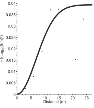
The experimental variogram (Fig. 8) was modelled using a Gaussian model with a sill equal to 0.05 (expressed in (log10 (S/m))²) and a range equal to 16.5 m (= ax). An arbitrary

anisotropy ax/az ratio of 5 was assumed (az = 3.3 m) to calculate the range in each direction

using equation 5.

We defined a reference model with a homogeneous resistivity value of 20 Ohm-m which is in the expected resistivity range for the clay layer found at ‒11 m, according to drillings. The structural constraint was imposed at the depth of the clay layer with βx/βz = 10.

We show the cumulative sensitivity matrix corresponding to the smoothness constraint solution in Fig. 1C. The sensitivity exhibits a classical pattern with a rapid decrease in depth and on the sides of the model. From the appraisal analysis performed in Caterina et al. (2013), it appeared that the first 5 m of soil is well-resolved and that, below ‒10 m, the image is not reliable quantitatively, which corresponds to a cumulative sensitivity of approximately 10-4. Below that level, the parameters show little sensitivity.

Several inversions were carried out with the selected constraints and results are presented in Fig. 9. Common features are present in the different models. First, the very resistive anomaly located at the surface from the abscissa 30 m to the end of the profile can be explained by the combination of effects due to the presence of roots (that part of the profile is located in woodland, see Fig. 7), and to the unsaturated sands. The second interesting anomaly is located more at depth and centreed at a distance of 20 m from the beginning of the profile. This latter anomaly is collocated with the expected source area of the contamination and can therefore be assumed as the contaminant plume. This assumption is confirmed by the electrical measurements made on the groundwater samples and illustrated in Fig. 7D, which clearly shows the presence of a more resistive fluid in the vicinity of the ‘contaminant’ anomaly. Depending on the chosen inversion scheme, the shape of the different anomalies varies. The smoothness constrained solution (Fig. 9A) tends to overestimate the thickness of the unsaturated root zone and produces a “contaminant plume” whose lateral extent (going from abscissas 5 m to 30 m) seems to be too small compared to the real extent of the contaminant plume (Fig. 7).

The shape of the anomaly obtained with the structural constraint (Fig. 9D) is more consistent with the expected behaviour of the contaminants. We also notice that the structural constraint has little influence on the parameters close to the top of the model. When we increase the

β

β

region above the clay layer remains almost the same as the one presented in Fig. 9D. In the clay layer, resistivities are almost homogeneous in the southern part of the model, but increase as we move to the north, which is not expected. The two regions are even more disconnected if we use a ratio

β

β

unrealistic (Fig. 9H).

The geostatistical solution (Fig. 9B) succeeds in reconstructing the thickness of the unsaturated zone in the northern part of the image. Moreover, the contaminant anomaly spreads over a larger area compared to the smoothness solution which is more consistent with the available chemical data (Fig. 7). However, at the location of the assumed contaminant source, the anomaly exhibits a sharp vertical resistivity contrast at a depth of –5 m as if there was some impervious layer (not met during drilling at that depth) preventing the downward migration of contaminants. Modifying the arbitrary ratio ax/az to a value of 3 has little impact

on the solution in this case (Fig. 9E).

The reference model solution (Fig. 9C) with a small closeness factor (α = 0.001) leads to almost no change in the unsaturated-root zone compared to the smoothness solution (Fig. 9A). In the saturated zone, the magnitude of the contaminant plume anomaly becomes slightly higher and spreads over a larger area. However, in the northern part of the model, the assumed contaminant plume seems to plunge below the clay layer which is geologically unrealistic. This can be corrected if we increase the resistivity value of the homogeneous reference model (= 50 Ohm-m) and the solution (Fig. 9F) becomes very similar to the one using a structural constraint (Fig. 9D).

The above presented results highlight the difficulty of choosing a type of regularization when ground truth data are lacking to validate the models. In that case, using a structural constraint with moderate

β

β

Contaminated site

The fourth case study presented is also located in Belgium. Due to confidentiality, we cannot give its exact location. The investigated area exhibits an underground contamination in chlorinated solvents (see Fig. 10). The source of the contamination is probably PCE which is found in some piezometers, but the component detected with the highest concentration is TCE. Similar to the Maldegem site, groundwater samples taken in the different piezometers suggest that natural degradation processes occur within the subsoil.

The geology encountered on the site can be decomposed into several units as revealed by borehole logs. First, we observe backfill deposits mainly composed of construction waste, carbonaceous waste and slags to a depth of ‒1 m. Backfills are not present on the whole ERT profile. Then, we observe Quaternary alluvial loams and colluvium on a thickness of 4 m. Below this layer, we find Tertiary geological materials composed of clayey sand and silty clay on a thickness of 8 m overlying a small layer of fine sands (≈ 1 m) and a layer of Tertiary clay whose thickness is 4 m. The underneath bedrock is made of limestone and is found at a depth of 18 m (see Fig. 10).

From a hydrogeological point of view, the contamination is located in an unconfined aquifer whose base is the Tertiary clay unit. No contamination was detected in the confined aquifer located in the limestone unit. The groundwater flow is directed from the southwest to the northeast.

Electrical resistance data were collected with 64 electrodes separated by 1.5 m using a Wenner-Schlumberger configuration with n spacing limited to 6 (944 measurements) and ‘a’ up to the maximum value of 18 m. The error was assessed using reciprocal measurements and an error model with an absolute value of 0.007 Ohm and a relative error of 1.7% was considered (Slater et al. 2000).

Due to a lack of independent resistivity data to compute variograms, no geostatistical information was available. The different drillings conducted on the site allow us to set a reference model and structural constraints. We defined a 2-layer reference model. The first layer has a homogeneous resistivity value of 30 Ohm-m and corresponds to the Quaternary/Tertiary deposits whereas the second layer, assimilated to the limestone, has a homogeneous resistivity value of 500 Ohm-m. The structure was imposed at the depth of the limestone bedrock (‒18 m) with βx/βz = 1000.

We show the cumulative sensitivity matrix corresponding to the smoothness constraint solution in Fig. 1D. Our knowledge of the site allows us to define a threshold on the cumulative sensitivity at 10-6. Below ‒20 m, the parameters become almost insensitive.

The smoothness solution (Fig. 11A) allows imaging of the backfill deposits close to the surface and characterized by high resistivities. As outlined previously, backfills are not present on the whole section which explains the discontinuities in the image. Below the backfills, we observe a very conductive zone that can be assimilated to the clayey Quaternary/Tertiary deposits. We do not expect a large resistivity contrast between the alluvial loams, clayey sands and clays. At the base of the model, we observe a more resistive zone that can be interpreted as the micritic limestone. However, this latter structure does not seem to have the same thickness on the whole section. We also observe a resistive anomaly that appears near the surface at the abscissa of 6 m and that plunges until a depth of ‒5 m (= groundwater table level). From that location, the anomaly seems to follow the groundwater flow direction (southwest to northeast) until the abscissa of 40 m where it is masked by the limestone structure. When we compare this anomaly with the chemical data (Fig. 10), we notice that the lateral extent and the location of the anomaly are quite similar to the detected contaminant plume. This suggests that the anomaly observed corresponds effectively to the contaminant plume. However, with the smoothness solution, it is difficult to assess its vertical

extent as resistivity contrasts are weak due to the smoothing, the presence of a resistive bedrock and the loss of resolution that occurs at depth.

The solution using a 2-layer reference model with α =0.05 (Fig. 11C) is sensibly different from the other ones and provides the best solution. The depth of the limestone is well retrieved, and their resistivity values are homogeneous. In the upper part of the model, no changes are observed in the backfills compared to the other solutions. The contaminant plume appears more clearly inside the Quaternary/Tertiary deposits, at least in the first half of the profile. In the middle of the profile, the assumed contaminant plume disappears completely for a very conductive area which could be caused by the presence of more biodegraded components and thus the presence of more Cl- ions in groundwater that tend to decrease bulk electrical resistivities. Between the contaminant anomaly and the limestone layer (abscissa between 5 m and 25 m), we observe an area with resistivity values larger than those expected for the lithology encountered (i.e., fine sands and clays) even with the effect of the reference model. This could be explained by the physical properties of the chlorinated solvents that are denser than water and that tend to plunge until they meet an impervious layer such as clay. However, the problem with that approach is that the solution may seem too close to the one expected a priori.

The structural solution (Fig. 11B) allows to correctly image the bedrock but provides few changes in the upper part compared to the smoothness solution (Fig. 11A).

Combining a structural constraint with a reference model (Fig. 11D) does not improve the solution compared to the one obtained with the use of the reference model alone (Fig. 11C).

Results presented on the 4 experimental sites allow us to draw some guidelines about the use of a priori information to enhance the quality of inverted models from the smoothness-constraint inversion. We will discuss them smoothness-constraint by smoothness-constraint.

Reference model solution

Adding a reference model in the solution is a straightforward incorporation of prior information. However, it is done through an additional weighting parameter which may be difficult to choose. With a low α value (equation 4), the reference model may have a relatively low impact on the solution and results may remain almost similar to the smoothness solution (Fig. 3A and 3D, Fig. 11A and 11D) or may significantly improve the results (Fig. 4A and 4C). With higher α values, the importance of the reference model increases and the solution begins to tend to the reference model (Fig. 3F). Low sensitivity areas are the first to be impacted by this effect. The optimization of the closeness factor is very difficult, even with borehole data (Fig. 4F).

Complex reference models with several layers or bodies should always be used carefully. It is similar to imposing both a structural constraint and the resistivity distribution of the solution. It may be too restrictive and compete with the data. The problem with this approach is that we may add too much information so that the solution obtained tends to the solution we expect a priori (Fig. 3H, Fig. 4H and Fig. 11C).

Consequently, the use of a reference model constraint with a large α value is well adapted only when information about the underground structure and resistivity distribution are well-known, which is rarely the case in practice. To impose sharp limits, it is safer to rely on the structural constraint.

When no information about the structure is available other than well information about the resistivity distribution, the use of a homogeneous reference model with a small value of α is indicated. The resistivity of the reference model may be chosen according to the expected resistivity at depth where the sensitivity is low, instead of choosing the mean apparent resistivity.

Structural inversion

Incorporating structural information can improve the solution, in some cases significantly. This is particularly true when the boundaries between the different underground structures are well-known and the resistivity contrast between them is well-marked (Fig. 3B and Fig. 11B). When the resistivity contrast is weak, the use of a structural constraint is not an efficient approach (Fig. 5B).

When dealing with structural constraint, we must moreover take care of the value of βx and βz

(equation 3) which are used to weight the gradients differently along each element boundaries of the inversion grid. High ratios βx/βz may lead to non-coherent coupling between the

different structure units (Fig. 9G and 9H). Low ratios act as softer constraints and should be used when there is uncertainty on the exact position of the boundary or when the expected resistivity contrast is low (Fig. 9D).

The structural constraint is thus particularly adapted to include limits such as bedrock or water table, for which resistivity variations are often observed. When these limit are not horizontal, the grid should be adapted to correspond with the structure (Doetsch et al. 2012).

Regularized geostatistical inversion

The geostatistical inversion may provide very consistent results and can significantly improve the solution compared to the other inversion approaches. However, it requires additional

measurements to sample the resistivity distribution and compute variograms (EM conductivity logs or water samples).

The method is not well adapted when a layered structure is expected, but yields results at least as good as the smoothness constraint (Fig. 3). When the distribution in resistivity does not display sharp contrasts, the improvement brought by the regularized geostatistical inversion is important (Fig. 4). Through the a priori covariance matrix, prior information will have a direct influence on all the parameters of the inverted model in a similar way as the smoothness constraint solution.

The choice of the prior model is also important and we recommend choosing it according to the expected resistivity at depth where the sensitivity is low.

According to our results, it seems that the role of the horizontal range is less crucial in surface ERT than the vertical range, which may be related to the sensitivity pattern of surface ERT, exhibiting a rapid decrease with depth (Hermans et al. 2012b). The method is less reliable when only the horizontal range is known (Fig. 9), even if it may help imaging the lateral extent of geological bodies. Conversely, it works fine when only the vertical range is known (Fig. 4).

CONCLUSION

We investigated three different approaches to incorporating prior information into the ERT inverse problem, namely reference model, structural constraint and regularized geostatistical inversion, and compared them to the standard smoothness constraint inversion.

In all cases, the results show that adding prior information in the inversion process led to a modification of the solution at least in zones of low sensitivity, i.e. at depth and on the sides of the section for surface arrays.

However, the choice of the constraint to apply is highly dependent on the type and amount of information available. A reference model can always be used, but its weight in the inversion process and its complexity are challenging to address. Several attempts are necessary to deduce, if possible, the best parameter to fit borehole measurements and there is no control on other parts of the model, which may lead to implausible solutions. It should then be used carefully to improve the smoothness constraint solution when there is not enough prior information to apply the other methods.

When the physical parameter (here electrical resistivity or conductivity) can be measured in several boreholes at different depths, the computation of a variogram is possible and a geostatistical constraint seems well suited. In addition to a proper prior model, this may be the method of choice to constrain the solution. However, in most cases, there will remain some uncertainty on the horizontal/vertical correlation length. The main advantage of this technique is to use borehole measurements only indirectly through the computation of a variogram. If the calculated variogram is representative of the whole site, the better correspondence observed in the boreholes is expected to be the same elsewhere in the section.

However, when lithological limits or other geophysical data sets are available and sharp contrasts expected, a structural constraint can be better suited. It enables us to disconnect, more or less according to the ratio between horizontal and vertical gradients, different lithological facies and creates sharp contrast whereas standard Occam inversion would lead to smooth transitions. Thus, it highlights better anomalies. This kind of constraint is often less strong than a complex reference model because it does not need to provide resistivity values before the inversion process.

Archie G.E. 1942. The electrical resistivity log as an aid in determining some reservoir characteristics. Transactions of the American Institute of Mining, Metallurgical and

Petroleum Engineers 146, 54‒62.

Aster R.C., Borchers B. and Thurber C. 2005. Parameter Estimation and Inverse Problems. Elsevier Academic Press, Amsterdam.

Blakely R.J. 1995. Potential Theory in Gravity and Magnetic Applications. Cambridge University Press, Cambridge.

Blaschek R., Hördt A. and Kemna A. 2008. A new sensitivity-controlled focusing regularization scheme for the inversion of induced polarization based on the minimum gradient support. Geophysics 73(2), F45‒F54.

Bouchedda A., Chouteau M., Binley A. and Giroux, B. 2012. 2-D joint structural inversion of cross-hole electrical resistance and ground penetrating radar data. Journal of Applied

Geophysics 78, 52‒67.

Cardarelli E. and Fischanger F. 2006. 2D data modelling by electrical resistivity tomography for complex subsurface geology. Geophysical Prospecting 54, 121‒133.

Chasseriau P. and Chouteau M. 2003. 3D gravity inversion using a model of parameter covariance. Journal of Applied Geophysics 52, 59‒74.

Constable S.C., Parker R.L. and Constable C.G. 1987. Occam's inversion: A practical algorithm for generating smooth models from electromagnetic sounding data. Geophysics 52, 289‒300.

Dahlin T. and Zhou B. 2004. A numerical comparison of 2D resistivity imaging with ten electrode arrays. Geophysical Prospecting 52, 379‒398.

Daily W.D., Ramirez A.L. and Johnson R. 1998. Electrical impedance tomography of a perchloroethelyne release. Journal of Environmental and Engineering Geophysics 2, 189– 201.

de Groot-Hedlin C. and Constable S. 1990. Occam’s inversion to generate smooth, two dimensional models from magnetotelluric data. Geophysics 55, 1613‒1624.

Doetsch J., Linde N., Coscia I., Greenhalgh S.A. and Green A.G. 2010. Zonation for 3D aquifer characterization based on joint inversions of multimethod crosshole geophysical data.

Geophysics 75(6), G53‒G64.

Doetsch J., Linde N., Pessognelli M., Green A.G. and Günther T. 2012. Constraining 3-D electrical resistance tomography with GPR reflection data for improved aquifer characterization. Journal of Applied Geophysics 78, 68‒76. doi:10.1016/j.jappgeo.2011.04.008.

Elwaseif M. and Slater L. 2010. Quantifying tomb geometries in resistivity images using watershed algorithms. Journal of Archaeological Science 37, 1424‒1436.

Farquharson C.G. and Oldenburg D.W. 1998. Nonlinear inversion using general measures of data misfit and model structure. Geophysical Journal International 134, 213‒227.

Gallardo L.A. and Meju M.A., 2003. Characterization of heterogeneous near-surface materials by joint 2D inversion of dc resistivity and seismic data. Geophysical Research

Letters 30(13), 1658–1661. doi: 10.1029/2003GL017370

Günther T. and Rücker C. 2006. A general approach for introducing information into inversion and examples from DC resistivity inversion. Near Surface 2006, Helsinki, Finland, Expanded Abstract, P039.

Halihan T., McDonald S.W. and Patey P. 2011. ERI evaluation of injectates used to remediate a dry cleaning site, Jackson, Tennessee. Symposium on the Application of

Geophysics to Engineering and Environmental Problems 24, 148.

Hermans T., Vandenbohede A., Lebbe L. and Nguyen F. 2012a. A shallow geothermal experiment in a sandy aquifer monitored using electric resistivity tomography. Geophysics 77(1), B11‒B21, doi:10.1190/GEO2011-0199.1.

Hermans T., Vandenbohede A., Lebbe L., Martin R., Kemna A., Beaujean J. and Nguyen F. 2012b. Imaging artificial salt water infiltration using electrical resistivity tomography constrained by geostatistical data. Journal of Hydrology _{438‒439, 168‒180.}

doi:10.1016/j.jhydrol.2012.03.021.

Hu W., Abubakar A. and Habashy T.M. 2009. Joint electromagnetic and seismic inversion using structural constraints. Geophysics 74(6), R99‒R109.

Johnson T.C., Routh P.S., Clemo T., Barrash W. and Clement W.P. 2007. Incorporating geostatistical constraints in nonlinear inversion problems. Water Resources Research 43, W10422. doi: 10.1029/2006WR005185.

Kaipio J.P., Kolehmainen V., Vauhkonen M. and Somersalo E. 1999. Inverse problems with structural prior information. Inverse Problems 15, 713‒729.

Kemna A. 2000. Tomographic inversion of complex resistivity – theory and application. PhD thesis. Ruhr-University of Bochum.

LaBrecque D.J., Miletto M., Daily W., Ramirez A. and Owen E. 1996. The effects of noise on Occam's inversion of resistivity tomography data. Geophysics 61(2), 538‒548.

Lelièvre P., Oldenburg D. and Williams N. 2009. Integrating geologic and geophysical data through advanced constrained inversions. Exploration Geophysics 40(4), 334‒341.

Linde N., Binley A., Tryggvason A., Pedersen L.B. and Révil A. 2006. Improved hydrogeophysical characterization using joint inversion of cross-hole electrical resistance and ground-penetrating radar traveltime data. Water Resources Research 42, W12404. doi: 10.1029/2006WR0055131

Loke M.H., Acworth I. and Dahlin T., 2003. A comparison of smooth and blocky inversion methods in 2D electrical imaging surveys. Exploration Geophysics 34, 182‒187.

Lucius J., Olhoeft G., Hill P. and Duke S. 1992. Properties and hazards of 108 selected substances. USGS Open-File Report 92–527.

Menke W. 1984. Geophysical Data Analysis: Discrete Inverse Theory. Elsevier, New-York.

Newmark R., Daily W.D., Kyle K.R. and Ramirez A.L. 1997. Monitoring DNAPL pumping using integrated geophysical techniques. Report UCRL-ID-122215. Livermore, Calif.: Lawrence Livermore National Laboratory.

Nguyen F., Garambois S., Jongmans D., Pirard E. and Loke M.H. 2005. Image processing of 2D resistivity data for imaging faults. Journal of Applied Geophysics 57, 260‒277.

Oldenburg D.W., McGillivray P.R. and Ellis R.G. 1993. Generalized Subspace Methods For Large-Scale Inverse Problems. Geophysical Journal International 114(1), 12‒20.

Oldenburg D.W. and Li Y. 1994. Subspace linear inverse method. Inverse Problems 10, 1‒21.

Pidlisecky A., Haber E. and Knight R. 2007. RESINVM3D: A 3D resistivity inversion package. Geophysics 72(2), H1‒H10.

Robert T., Dassargues A., Brouyère S., Kaufman O., Hallet V. and Nguyen F. 2011. Assessing the contribution of electrical resistivity tomography (ERT) and self-potential

methods for a water well drilling program in fractured/karstified limestones. Journal of

Applied Geophysics 75(1), 42‒53.

Saunders J.H., Herwanger J.V., Pain C.C. and Wothington M.H. 2005. Constrained resistivity inversion using seismic data. Geophysical Journal International 160, 785‒796.

Schön J.H. 2004. Physical Properties of Rock. In: Physical Properties of Rock, Vol. 18 (ed. E.K. Helbig and S.Treitel). Elsevier.

Scott J.B.T., Barker R.D. and Peacock S. 2000. Combined seismic refraction and electrical imaging. 6th Meeting of the European Association for Environmental and Engineering Geophysics, Bochum, Germany, Expanded Abstract, EL05.

Slater L., Binley A.M., Daily W. and Johnson R. 2000. Cross-hole electrical imaging of a controlled saline tracer injection. Journal of Applied Geophysics 44, 85‒102.

Tikhonov A.N. and Arsenin V.A. 1977. Solution of Ill-posed Problems. Winston & Sons, Washington.

Vandenbohede A., Lebbe L., Gysens S., Delecluyse K. and DeWolf P. 2008. Salt water infiltration in two artificial sea inlets in the Belgian dune area. Journal of Hydrology 360, 77‒86.

Vandenbohede A., Hermans T., Nguyen F. and Lebbe L. 2011. Shallow heat injection and storage experiment: heat transport simulation and sensitivity analysis. Journal of Hydrology 409, 262‒272. doi:10.1016/j.jhydrol.2011.08.024

Wijns C., Boschetti F. and Moresi L. 2003. Inverse modelling in geology by interactive evolutionary computation. Journal of Structural Geology 25, 1615‒1621. doi:10.1016/S0191-8141(03)00010-5

Yeh T.-C.J., Liu S., Glass R.J., Baker K., Brainard J.R., Alumbaugh D. and LaBrecque D. 2002. A geostatistically based inverse model for electrical resistivity surveys and its applications to vadose zone hydrology. Water Resource Research 38(12). doi: 10.1029/2001WR001204.

Yeh T.-C.J., Zhu J., Englert A., Guzman A. and Flaherty S. 2006. A successive linear estimator for electrical resistivity tomography. In: Applied Hydrogeophysics, (eds H. Vereecken, A. Binley, G. Cassiani, A. Revil and K. Titov). NATO Science Series, Springer.

FIGURES

FIGURE 1. Cumulative sensitivity matrix for (A) the Ghent site, (B) the Westhoek site, (C) the Maldegem site and (D) the contaminated site. All images present the same pattern with a decrease of sensitivity at depth and on the sides of the models. (B) and (D) were extended to an important depth to highlight the effect of the incorporation of prior information in zones of very low sensitivity.

0 10 20 30 40 −10 −8 −6 −4 −2 0 X (m) Y (m)

A) Ghent site Log10 S

−7 −6 −5 −4 −3 −2 −1 0 0 50 100 150 200 −25 −20 −15 −10 −5 0 5 10 X (m) Y (m)

B) Westhoek site Log10 S

−8 −6 −4 −2 0 0 20 40 60 −15 −10 −5 0 X (m) Y (m)

C) Maldegem site Log10 S

−7 −6 −5 −4 −3 −2 −1 0 0 20 40 60 80 −30 −25 −20 −15 −10 −5 0 X (m) Y (m)

D) Contaminated site Log10 S

−8 −6 −4 −2 0

FIGURE 2. EM39 measurements (A) and vertical variogram (B) of the Ghent site. The horizontal limits in (A) are derived from borehole logs. EM39 measurements were used to derive the vertical correlation length of the logarithm of the resistivity. The model best fitting the data is a spherical model with sill value equal to 0.05 and a vertical range of 2.4 m.

FIGURE 3. Inversions for the Ghent Site. (A) The smoothness constrained solution shows a general transition from high to low resistivity. (B) The structural inversion is very consistent with available a priori information (three layers). (C) The regularized geostatistical inversion describes three zones but not horizontal. (D) The solution with a reference model (α = 0.05) is close to the smoothness-constrained solution. (E) The regularized geostatistical inversion with doubled ax is not highly different. (F) The solution with a reference model with

increased weight (α = 0.5) tends to the structural inversion. (G) The regularized geostatistical inversion with a bad prior model yields implausible results in the low sensitivity zone. (H) The solution with a bad reference model (α = 0.5) yields implausible results.

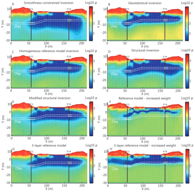
FIGURE 4. Inversions for the Westhoek site from southwest to northeast. (A) The smoothness-constrained solution spreads the sea water intrusion on a big thickness. (B) The regularized geostatistical inversion limits this thickness giving a contrast in resistivity closer to the reality. (C) The smoothness constrained solution with a homogeneous reference model (α = 0.05) is improved. (D) The structural inversion with a structure at the top of the clay seems to produce undesirable features in the section at the imposed location. (E) Structural inversion with a structure at the bottom of the clay yields a more plausible solution. (F) The smoothness constrained solution with a homogeneous reference model with increased weight (α = 0.5) reduces the thickness of infiltrated sea water. (G) The smoothness constrained

Clay Clay Clay Clay Clay Clay Clay Clay

solution with a 3-layer reference model (α = 0.05) does not improve the solution. (H) The smoothness constrained solution with a 3-layer reference model and increased weight (α = 0.5) brought an improvement.

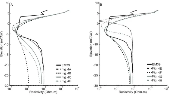
FIGURE 5. Comparisons of calculated conductivity with EM conductivity measurements in P12, located at abscissa 57 m on the profile. (A) shows the solutions of Fig. 4 A to D and (B) shows the solutions of Fig. 4 E to H.

FIGURE 6. Comparisons of calculated conductivity with EM conductivity measurements in P18, located at abscissa 167 m on the profile. (A) shows the solutions of Fig. 4 A to D and (B) shows the solutions of Fig. 4 E to H.

FIGURE 7. Contaminated site of Maldegem. The contamination took place at the location of the former laundry. Due to the groundwater flow directed towards north-east, contaminants are now found up to piezometers PB504 and PB501 (A, B and C). Chemical data show that natural attenuation occurs on the site. A correlation seems to exist between the resistivities derived from groundwater samples and the presence of contaminants. Samples showing advanced degradation generally are located in zones exhibiting slightly lower resistivity than those in the source area (D). This is consistent with the fact that a Cl- ion is released in the groundwater each time a chlorinated solvent molecule is degraded into a by-product, leading

to a general decrease of water resistivity. The ERT profile, composed of 72 electrodes spaced at 1 m, was set up in order to cross the main contaminated area and to be parallel to the groundwater flow direction.

FIGURE 8. Horizontal variogram of the Maldegem site. Groundwater conductivity measurements were first converted to bulk resistivities and then used to derive the horizontal correlation length of the logarithm of the resistivity. The model best fitting the data is a Gaussian model with a sill value equal to 0.04 and a vertical range of 16.5 m.

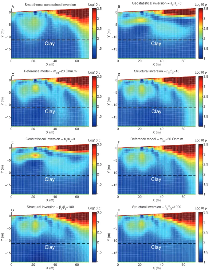
FIGURE 9. Inversions for the Maldegem site from the south-west to the north-east. The smoothness-constrained solution (A) tends to overestimate the thickness of the unsaturated zone and limits the lateral extent of the assumed contaminant anomaly. The regularized

geostatistical inversion (B) succeeds in reconstructing these features but the contaminant anomaly seems to be a little too flattened at the source. Adding a reference model (C) spreads the shape of the contaminant anomaly over a large section tending to plunge below the clay barrier. Adding a structure at the top of the clay layer (D) produces mainly changes in the contaminant anomaly shape limited at depth by the clay layer. Changing the vertical range for the geostatistical inversion (E) has relatively little impact on the solution. Modifying the value of the homogeneous reference model (F) slightly changes the shape of the contaminant anomaly, particularly in the northern side of the model. Imposing sharper structural constraints (G: βx/βz = 100 and H: βx/βz = 1000) at the sand-clay boundary do not modify

greatly the shape and magnitude of the anomalies present in the upper part of the model but tend to produce discontinuities between the two geological bodies.

FIGURE 10. Schematic cross-section of the contaminated site (Belgium). The contaminants detected on the site are chlorinated solvents. The groundwater flow is directed towards north-east. A delineation of the contaminant plume is proposed based on available chemical data and on (hydro)geological knowledge. The ERT profile, composed of 64 electrodes spaced of 1.5 m, was set up in order to cross the main contaminated area and to be parallel to the groundwater flow direction.