HAL Id: hal-00426435
https://hal.archives-ouvertes.fr/hal-00426435
Submitted on 26 Oct 2009
HAL is a multi-disciplinary open access
archive for the deposit and dissemination of
sci-entific research documents, whether they are
pub-lished or not. The documents may come from
teaching and research institutions in France or
abroad, or from public or private research centers.
L’archive ouverte pluridisciplinaire HAL, est
destinée au dépôt et à la diffusion de documents
scientifiques de niveau recherche, publiés ou non,
émanant des établissements d’enseignement et de
recherche français ou étrangers, des laboratoires
publics ou privés.
Rough thin pavement thickness estimation by GPR
Nicolas Pinel, Cédric Le Bastard, Limei Liu, Christophe Bourlier, Yide Wang
To cite this version:
Nicolas Pinel, Cédric Le Bastard, Limei Liu, Christophe Bourlier, Yide Wang. Rough thin pavement
thickness estimation by GPR. International Geoscience and Remote Sensing Symposium, Jul 2009, Le
Cap (Cape Town), South Africa. pp.1255. �hal-00426435�
ROUGH THIN PAVEMENT THICKNESS ESTIMATION BY GPR
N. Pinel, L. Liu, C. Bourlier, Y. Wang
IREENA Laboratory, Universit´e de Nantes
Polytech’Nantes
Nantes, France
C. Le Bastard
LRPCA
ERA 17
Les Ponts de C´e, France
ABSTRACT
In civil engineering, usually the methods used to estimate the thickness of thin pavements consider flat interfaces for simpli-fication. In this paper, the roughness of the surfaces is taken into account. First, the amplitudes of the first two echoes from the rough thin pavement are calculated from a rigorous electromagnetic method, the PILE method. A comparison is then made with the flat interface case, and their differences in the electromagnetic backscattering are highlighted. Eventu-ally, the influence of the pavement roughness on the pavement thickness estimation is investigated by using the Maximum Likelihood Method.
Index Terms— Radar scattering, Electromagnetic
scat-tering by rough surfaces, Ground wave propagation, Nonde-structive testing, Delay estimation
1. INTRODUCTION
Ground penetrating radar (GPR) is a useful means of me-dia sounding, which is widely used at centimeter-scale wave-lengths in road surfaces evaluation [1, 2, 3]. In this context, the roadway is usually considered as made up of perfectly flat stratified interfaces. Then, the vertical structure of the road-way is deduced from radar echo detection and amplitudes es-timation. Echo detection provides the time-delay estimation (TDE) associated with each interface, and amplitude estima-tion is used to retrieve the wave speed within each layer. The case of small pavement thicknesses was studied in a recent paper [3].
In general, classical methods of pavement thickness esti-mation assume flat interfaces for the pavement. Even if this first approximation has sense and is rather realistic, to our knowledge the validity domain of this approximation, and its influence on the electromagnetic backscattering and on the GPR process have not been studied in details. This is the scope of this work. Thus, in this paper, the surface roughness of the pavement is taken into account in the electromagnetic backscattering modeling and in the GPR thickness estimation process, and compared with the case of neglecting the rough-ness of the pavement.
First, the amplitudes of the first two echoes from the rough thin pavement are calculated with a rigorous electromagnetic method, namely the PILE method [4]. The frequency behav-ior of the echoes is then presented in the considered frequency band,f ∈ [1.0; 3.0] GHz, comparatively to the echoes
ob-tained for flat interfaces. Finally, the influence of the pave-ment roughness on the thickness estimation is investigated by using the Maximum Likelihood Method.
2. ECHO AMPLITUDES: FREQUENCY BEHAVIOR
In this section, the frequency behavior of the first two backscattered echoess1ands2of a rough pavement is
pre-sented. To calculate the echoes within the frequency band
f ∈ [1.0; 3.0] GHz, the PILE (Propagation Inside Layer
Expansion) method [4] is used. It is a Method-of-Moments based method which is able to compute rigorously each echo reflected by a flat or a rough layer.
2.1. Simulation parameters
The pavement under study is an Ultra Thin Asphalt Surfacing (UTAS) of thickness H = 20 mm [5], overlying a rolling
band of same general composition. It is assumed that the UTAS and the rolling band can be assimilated to homoge-neous media at the frequency band under studyf ∈ [1.0; 3.0]
GHz [3, 6, 7]. Their relative permittivities typically range be-tween4 and 8 [8], and their conductivities between 10−3and
10−2 S/m [9]. For the simulations, their relative
permittivi-ties are taken asǫr2 = 5 and ǫr3 = 8, respectively, and their
conductivities asσ2 = 5 × 10− 3
S/m andσ3 = 10− 2
S/m, respectively. The two rough interfaces ΣA andΣB are
as-sumed to be described by a Gaussian height probability den-sity function (pdf), and an exponential auto-correlation func-tion [10, 11]. For the upper interface ΣA, the root mean
square (rms) heightσhAis of the order of1 mm, and the
cor-relation lengthLcAof the order of5 − 10 mm. For the lower
interfaceΣB, the rms heightσhB and the correlation length
LcB are a bit greater. For the simulations, the chosen
param-eters areσhA= 0.8 mm, LcA = 10.0 mm, σhB = 1.6 mm,
only very weakly correlated, so that it can be assumed here that they are statistically uncorrelated.
Concerning the incident wave, a monochromatic incident wave of TM polarization (also called vertical polarization) is considered, with normal incidence onto the pavement,θi= 0.
The emitter antenna is assumed to be in the far-field zone of the ground, so that the incident wave is assumed to be plane. The typical width of the central zone illuminated by the emitter antenna is of the order of100 − 200 mm [12].
Then, for the simulations of the numerical method, surfaces of lengthL = 600 mm will be considered, illuminated by
a Thorsos beam of attenuation parameterg = L/6. A
nor-mal incident wave (with incidence angleθi = 0) is taken,
and the first two orders of the reflected echoes by the rough layers1ands2are calculated under the PILE method. Then,
to determine the frequency behavior of the received echoes
sk ≡ sk(f ) (see equation (2) of [3]) in the backscattering
directionθs = θi = 0, it is necessary to run the numerical
simulation scenario at different frequenciesf within the
con-sidered bandwidth,f ∈ [1.0; 3.0] GHz.
The numerical process is described as follows. The rough layer, with two independent rough surfaces, is generated by a Monte-Carlo process (the two rough surfaces being generated from independent processes), for which the calculation of the backscattered signalss1ands2is led with the PILE. In order
to study the variability of the echo amplitudess1ands2,
sev-eral independent Monte-Carlo processes are generated. Thus, it is possible to estimate the standard deviations of the echo amplitudes, and even a profile of their calculated probability density functions if a significant number of realizations is led (typically, of the order of 10000 [13]). Indeed, for a
prac-tical scenario, the illuminated surface area is of the order of
100 − 200 mm, which is not large in comparison with the two
surface correlation lengthslcA = 10.0 mm and lcB = 30.0
mm. This implies that the received echo amplitudes depend on the location of the pavement where the measurement is made. As a consequence, in order to study the variability of the received echo amplitudes, a significant number of realiza-tions must be generated.
To compute the numerical results, at least1000
indepen-dent realizations of a Monte-Carlo process are generated, in order to simulate the variability of the received echoes. For the simulation of the numerical method, the two rough inter-faces are sampled with a sampling step∆x = λ2/10, with λ2
the wavelength inside the inner mediumΩ2.
2.2. Numerical results
First, numerical simulations are led at a fixed radar frequency
f , in the middle of the radar band under study, i.e. f = 2.0
GHz. In order to study the probability density function (pdf) of the echoes s1 and s2, the number of realizations of the
Monte-Carlo process is taken as10000. A comparison is also
made between the case with rough interfaces and the case
0.3780 0.38 0.382 0.384 200 400 600 800 1000 1st echo s 1 − Real part −0.050 0 0.05 200 400 600 800 1000 1st echo s 1 − Imaginary part 0.3780 0.38 0.382 0.384 200 400 600 800 1000 1st echo s 1 − Modulus −50 0 5 200 400 600 800 1st echo s 1 − Phase (deg.)
Fig. 1. Probability density functions (pdf) of the first echo s1 (real part, imaginary part, modulus and phase) obtained
from10000 realizations, at a radar frequency f = 2 GHz.
The mean value is plotted in red dashed vertical line, and the mean value plus and minus the standard deviation are plotted in purple dashed vertical line. Then, the pdf is compared with a Gaussian pdf having the same mean value and standard de-viation. Comparison is also made with the flat case in green vertical line. 0.060 0.08 0.1 0.12 200 400 600 800 1000 1200
2nd echo s2 − Real part
−0.050 0 0.05 200 400 600 800 1000 1200
2nd echo s2 − Imaginary part
0.080 0.09 0.1 0.11 200 400 600 800 1000 1200 2nd echo s 2 − Modulus −500 0 50 200 400 600 800 1000 1200 2nd echo s 2 − Phase (deg.)
Fig. 2. Same simulation parameters as in Fig. 1, but for the
second echos2
with flat interfaces. Numerical results of the simulated pdfs are plotted in Fig. 1 for the first echos1, and in Fig. 2 for the
second echos2. In each figure, the pdf of the real part, the
imaginary part, the modulus, and the phase (in degrees) of the echo are represented. The mean value is plotted in red dashed vertical line, and the mean value plus and minus the standard deviation are plotted in purple dashed vertical line. Then, the
1 1.5 2 2.5 3 0.375 0.38 0.385 1st echo s 1
Real part of the echo
Flat case
Rough case (µ)
Rough case (µ ± 2σ)
Rough case (1 real.)
1 1.5 2 2.5 3 0.08 0.09 0.1 2nd echo s 2 Radar frequency f (GHz)
Real part of the echo
Flat case
Rough case (µ)
Rough case (µ ± 2σ)
Rough case (1 real.)
Fig. 3. Frequency behavior of the real part of the first two
echoess1ands2
pdf is compared with a Gaussian pdf having the same mean value and standard deviation in full red line. A comparison is also made with the case of flat interfaces (whose pdf is a Dirac delta function) in green vertical line.
Concerning the first echos1, the imaginary part and the
phase do not highlight a significant difference between the flat case and the mean value of the rough case. Moreover, the dispersion around this mean value remains low: for instance, in the phase distribution, the RMS phase is of the order of1
degree. By contrast, a relatively small but though significant difference occurs in the real part and in the modulus. As ex-pected, the (upper) surface roughness induces a decrease of the echo (real part or modulus) comparatively to the flat case. However, this decrease remains small owing to the small elec-tromagnetic roughness of the surface at this typical frequency. Moreover, the dispersion around this mean value remains low. The general shape of the pdf resembles a Gaussian for the imaginary part and the phase. For the real part and the mod-ulus, the shape differs only slightly from a Gaussian, and is assimilated to a Gaussian as well in first approximation.
The same qualitative observations can be made for the second echos2. In this case, the relative differences between
the flat case and the mean value of the rough case are higher, owing to the larger electromagnetic roughness of the layer.
Second, in what follows the frequency behavior of the echoess1 ands2 is investigated in the whole range of the
two radar frequency bands under study, i.e. forf ∈ [0.5; 3.0]
GHz, for which1000 Monte-Carlo processes were used.
Fig. 3 presents the frequency behavior of the real part of the first two echoess1 ands2. The flat case is plotted in
green full line, the mean value of the rough case in red circled dashed line, the mean value plus or minus twice the standard deviation of the rough case in magenta circled dash-dot line,
10 15 20 25 30 35 40 45 10−3 10−2 10−1 100 101 102 RRMSE (%) SNR (dB) T
1, flat layer case
T
1, rough layer case
T2, flat layer case T2, rough layer case H, flat layer case H, rough layer case
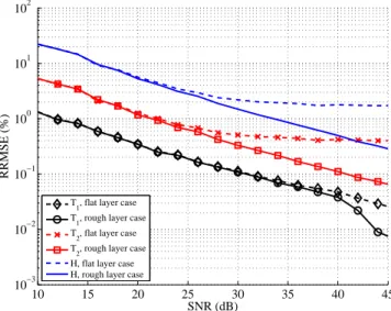
Fig. 4. RRMSE variations on the two estimated time delays ˆ
T1and ˆT2, as well as on the layer thickness ˆH, vs. the SNR
and one realization of the rough case in blue dotted line with plus signs. The results highlight that as the radar frequency in-creases, the amplitudes of the backscattered echoess1ands2
decrease, because the layer (electromagnetic) roughness in-creases relatively to the wavelength. Moreover, for the lower frequenciesf ≈ 1 GHz, it can be seen that the difference
with the flat case is relatively weak and could be neglected. On the contrary, for the higher frequenciesf ≈ 3 GHz, the
relative difference with the flat case is significant and cannot be neglected any more, as it exceeds10 percent for instance
fors2. Thus, significant differences appear in the
backscat-tered echoess1 ands2 between the rough and flat cases, in
particular for the higher frequencies.
Then, let us have a look at the consequences of these dif-ferences in the electromagnetic backscattering on the thick-ness estimation by GPR, with the Maximum Likelihood Method (MLM).
3. THICKNESS ESTIMATION BY GPR
The process to determine the time delays of the first two echoes is explained in details in [3]. To perform time delay estimation (TDE), the MLM is used. An additive complex Gaussian white noise is considered to model the measurement uncertainties and the noise in the instruments. The radar pulse is a ricker pulse, defined as the second derivative of a Gaus-sian pulse. The data vector is made of5 samples within the 2
GHz frequency bandwidth (see Fig. 3). The scenario under study is the same as described in the previous section. Thus, the data (i.e., the echo amplitudess1ands2) used to
deter-mine the time delays correspond to the realization plotted in blue dotted line with plus signs in Fig. 3.
(RRMSE) variations on the two estimated time delays ˆT1and
ˆ
T2, as well as on the layer thickness ˆH, vs. the signal-to-noise
ratio (SNR), for the frequency bandf ∈ [1.0; 3.0] GHz. First,
for both flat and rough cases, it can be seen that the RRMSE decreases with increasing SNR. A difference between the flat and rough cases is observable in ˆT1for SNR higher than40
dB, in ˆT2 for SNR higher than 25 dB, and in ˆH for SNR
higher than25 dB.
As a consequence, taking the roughness of the surfaces into account makes it possible to increase the performances of the algorithm for moderate to high SNR. Thus, in the context of high SNR, it is important to take the roughness into account in the data modeling to obtain very low RRMSE, and this modeling allows in this case an even better precision of the thickness estimation. On the other hand, for low SNR and/or for a first estimate of the pavement thickness, these results confirm that taking the surface roughness into account is not necessary: this phenomenon can be neglected in this other context, as usually done in many previous studies.
4. CONCLUSION
In conclusion, taking the surface roughness into account in the pavement thickness estimation by standard GPR of bandwidth of the order of2 GHz allows us to quantify the classical
ap-proximation which considers flat interfaces. Thus, for typical pavements encountered in practice, like hereB = [1.0; 3.0]
GHz in Fig. 4, the difference between the rough and the flat cases in the backscattered echoes amplitudes is significant for the higher frequencies of the bandwidth. Then, the influence of this difference in the GPR estimation process is significant for moderate to high SNR (typically,25 dB for the thickness).
As a consequence, taking the roughness into account in the data model is of interest, and this modeling allows a better precision in the thickness estimation process.
5. REFERENCES
[1] X. D´erobert, C. Fauchard, P. Cˆote, E. Le Brusq, E. Guil-lanton, J.Y. Dauvignac, and C. Pichot, “Step-frequency radar applied on thin road layers,” Journal of Applied
Geophysics, vol. 47, no. 3, pp. 317–325, July 2001.
[2] J.S. Lee, C. Nguyen, and T. Scullion, “A novel, com-pact, low-cost, impulse ground-penetrating radar for nondestructive evaluation of pavements,” IEEE
Trans-actions on Instrumentation and Measurement, vol. 53,
no. 6, pp. 1502–9, Dec. 2004.
[3] C. Le Bastard, V. Baltazart, Y. Wang, and J. Saillard, “Thin-pavement thickness estimation using GPR with high-resolution and superresolution methods,” IEEE Transactions on Geoscience and Remote Sensing, vol.
45, no. 8, pp. 2511–19, Aug. 2007.
[4] N. D´echamps, N. de Beaucoudrey, C. Bourlier, and S. Toutain, “Fast numerical method for electromagnetic scattering by rough layered interfaces: Propagation-inside-layer expansion method,” Journal of the Optical
Society of America A, vol. 23, no. 2, pp. 359–69, Feb.
2006.
[5] “AFNOR standard NFP 98-137,” 1992, French stan-dard.
[6] U. Spagnolini, “Permittivity measurements of multilay-ered media with monostatic pulse radar,” IEEE
Trans-actions on Geoscience and Remote Sensing, vol. 35, no.
2, pp. 454–63, Mar. 1997.
[7] G.G. Gentili and U. Spagnolini, “Electromagnetic in-version in monostatic ground penetrating radar: TEM horn calibration and application,” IEEE Transactions
on Geoscience and Remote Sensing, vol. 38, no. 4, pp.
1936–46, July 2000.
[8] M. Adous, X. D´erobert, and P. Qu´eff´elec, “EM charac-terization of bituminous concretes in a large frequency bandwidth: First results,” in The 11th International
Conference on Ground Prenetrating Radar, Ohio, USA,
June 2006.
[9] C. Fauchard, Utilisation de Radars tr`es hautes fr´equences : Application `a l’auscultation non destruc-tive des chauss´ees, Ph.D. thesis, University of Nantes,
France, 2001.
[10] E.S. Li and K. Sarabandi, “Low grazing incidence millimeter-wave scattering models and measurements for various road surfaces,” IEEE Transactions on
An-tennas and Propagation, vol. 47, no. 5, pp. 851–61, May
1999.
[11] F. Koudogbo, P.F. Combes, and H.-J. Mametsa, “Nu-merical and experimental validations of IEM for bistatic scattering from natural and manmade rough surfaces,”
Progress In Electromagnetics Research, vol. 46, pp.
203–244, 2004.
[12] F. Liu, Mod´elisation et Exp´erimentation Radar
Impul-sionnel et ´a Sauts de Fr´equence Pour lAuscultation de Milieux Stratifi´es du G´enie Civil, Ph.D. thesis,
Univer-sity of Nantes, France, Apr. 2007.
[13] R. Duss´eaux and R. De Oliveira, “Effect of the illumi-nation length on the statistical distribution of the field scattered from one-dimensional random rough surfaces: analytical formulae derived from the small perturbation method,” Waves in Random and Complex Media, vol. 17, no. 3, pp. 305–20, Aug. 2007.