Using Problem Structure in Derivative-free Optimization

RESEARCH OUTPUTS / RÉSULTATS DE RECHERCHE

Author(s) - Auteur(s) :

Publication date - Date de publication :

Permanent link - Permalien :

Rights / License - Licence de droit d’auteur :

Bibliothèque Universitaire Moretus Plantin

Dépôt Institutionnel - Portail de la Recherche

researchportal.unamur.be

University of Namur

Using Problem Structure in Derivative-free Optimization

Toint, Philippe

Published in:

SIOPT Views and News

Publication date:

2006

Document Version

Early version, also known as pre-print

Link to publication

Citation for pulished version (HARVARD):

Toint, P 2006, 'Using Problem Structure in Derivative-free Optimization', SIOPT Views and News, vol. 17, no. 1, pp. 11-18.

General rights

Copyright and moral rights for the publications made accessible in the public portal are retained by the authors and/or other copyright owners and it is a condition of accessing publications that users recognise and abide by the legal requirements associated with these rights. • Users may download and print one copy of any publication from the public portal for the purpose of private study or research. • You may not further distribute the material or use it for any profit-making activity or commercial gain

• You may freely distribute the URL identifying the publication in the public portal ?

Take down policy

If you believe that this document breaches copyright please contact us providing details, and we will remove access to the work immediately and investigate your claim.

Articles

Using Problem Structure in

Derivative-free Optimization

1.

Introduction

Derivative-free optimization is the branch of opti-mization where the minimizer of functions of several variables is sought without any use of the objective’s derivatives. Although a number of problems may in-volve constraints, we will focus in this paper on the unconstrained case, i.e.,

min

x∈Rnf (x), (1)

where f is an objective function which maps Rninto R and is bounded below, and where we assume that the gradient of f (and, a fortiori, its Hessian) cannot be computed for any x.

The main motivation for studying algorithms for solving this problem is the remarkably high demand from practitioners for such tools. In most of the case known to the author, the calculation of the objective function value f (x) is typically very expensive, and its derivatives are not available either because f (x) results from some physical, chemical or econometri-cal measure, or, more commonly, because it is the result of a possibly very large computer simulation, for which the source code is effectively unavailable. The occurrence of problems of this nature appears to be surprisingly frequent in the industrial world. For instance, we have heard of cases where evaluating f (x) requires the controlled growth of a particular crop or the meeting of an adhoc committee. As can be guessed from this last example, the value of f (x) may in practice be contaminated by noise, but the numerical techniques for handling this latter charac-teristic are also outside the scope of our presentation.

Several classes of algorithms are known for derivative-free optimization. A first class is that of direct search techniques, which includes the well-known and widely used simplex reflection algorithm of [22] or its modern variants [11, 27], the old Hookes and Jeeves method [20] or the parallel direct search algorithm initiated by Dennis and Torczon [15, 29]. These methods are based on a predefined geometric pattern or grid and use this tool to decide where the objective function should be evaluated. A recent and comprehensive survey of the development in this class is available in [21] and the associated bibliography is accessible at http://www.cs.wm.edu/˜va/research/wilbur.html. See also the paper by Abramson, Audet and Dennis in this issue. The main advantage of methods in this class is that they do not require smoothness (or even continuity) of the objective function.

A second algorithmic class of interest is that of in-terpolation/approximation techniques pioneered by Winfield [30, 31] and by Powell in a series of pa-pers starting with [23, 24]. In these methods, a low-order polynomial (linear or quadratic) model of the objective function is constructed and subsequently minimized, typically in a trust-region context (see [6, Chapter 9]). Because they build smooth models, they are appropriate when the objective function is known to be smooth. A common feature of the al-gorithms of this type is that they construct a basis of the space of suitable polynomials and then derive the model by building the particular linear combi-nation of the basis polynomials that interpolate (or sometimes approximate) known values of f (x). Pow-ell favors a basis formed of Lagrange fundamental polynomials, while Conn et al. [7, 8, 10] use New-ton fundamental polynomials instead. Both choices have their advantages and drawbacks, which we will not discuss here. The polynomial space of interest is typically defined as the span of a given set of mono-mials: full quadratic polynomials in the two vari-ables x1 and x2 are for instance those spanned by 1, x1, x2, x1x2, x21 and x22.

While methods in these two classes have been studied and applied in practice, their use has re-mained essentially limited to problems involving only a very moderate number of variables: the solu-tion of problems in more than 20 variables is indeed possible in both cases, but is typically very

compu-tationally intensive. In direct search techniques, this cost is caused by the severe growth in the number of grid or pattern points that are necessary to “fill” R20 or spaces of even higher dimensions. A simi-lar difficulty arises in interpolation methods, where a total of (n + 1)(n + 2)/2 known function values are necessary to define a full quadratic model, but it is also compounded with the relatively high com-plexity in linear algebra due to repetitive minimiza-tion/maximization of such quadratic polynomials. One may therefore wonder if there is any hope for the derivative-free solution of problems in higher dimen-sions. It is the purpose of this paper to indicate that this hope may not be unfunded, at least for problems that exhibits some structure. Section 2 discusses the partially separable structure which will be central here, while Sections 3 and 4 indicate how it can be numerically exploited in direct search and interpo-lation methods, respectively. We then consider the special case of sparse problems in Section 5. Some conclusions are finally presented in Section 6.

2.

Problem structure

Large-scale optimization problems often involve dif-ferent parts, or blocks. Each block typically has its own (small) set of variables and other (small) sets of variables that link the block with other blocks, re-sulting, when all blocks are considered together, in a potentially very large minimization problem. One may think, for instance, of a collection of chemi-cal reaction tanks, each with its temperature, pres-sure or stirring controls, and with its input raw material and output products. Other examples in-clude discretized problems where a given node of the discretization may involve more than a single variable but is only connected to a few neighbour-ing nodes, or PDE problems with domain decom-position, or multiple-shooting techniques for trajec-tory/orbit calculations, where each orbital arc only depends on a few descriptive or control variables, with the constraint that the different arcs connect well via a (small) set of common variables. Exam-ples of this type just abound, especially when the size of the problem grows. It is interesting that their structure can very often be captured by the notion of partial separability, introduced by Andreas Griewank and the author in [17, 19].

A function f : Rn → R is said to be partially separable, if its value may be expressed, for every x, as f (x) = q X i=1 fi(Uix), (2)

where each element function fi(x) is a function de-pending on the internal variables Uix with Ui being a ni × n matrix (ni  n). Very often, the matrix Ui happens to be a row subset of the the identity matrix, and the internal variables are then just a (small) subset of the original problem variables.

Griewank and Toint show in [18] that every twice-continuously differentiable function with a sparse Hessian is partially separable, which gives a hint at why such functions are so ubiquitous. It is remark-able that, although this is only an existence result and specifies a particular decomposition (2) only in-directly, we are not aware of any practical problem having a sparse Hessian and whose partially separa-ble decomposition is not explicitly known.

Partially separable functions (and their extension to group-partially separable ones) have been instru-mental in the design of several numerical codes, in-cluding the LANCELOT package [5]. We now intend to show how they can be exploited in derivative-free optimization.

3.

Direct search for partially

sep-arable objective functions

For our description of the structure use in direct search methods, we focus on the common case where the matrices Ui are subsets of the identity, which then implies that each element function fi only de-pends on a small subset of the problem variables. As in [28], we assume that each fi is available individ-ually, along with a list of the problem variables on which fi depends. Two problem variables are then said to interact if at least one element fi depends on both. Sets of non-interacting variables are useful because the change in f from altering all variables in the set is just the sum of the changes in f arising from altering each variable in the set individually.

Exploiting partial separability is advantageous for direct search methods in two separate ways. It can both reduce the computational cost of each function

value sought, and also provide function values at re-lated points as a by-product. For example, consider a totally separable function

f (x) = n X

i=1 fi(xi)

where x = (x1, . . . , xn)T, and where the value of each element fi is known at a point x. Assume, as is typical in pattern search methods, that we wish to explore f in the vicinity of x by calculating f at each point of the form {x ± hei}ni=1, where h is a positive constant and ei is the ith column of the identity matrix. Calculating f at each point requires the evaluation of one fi, and so the total cost of the 2n function values at the points {x±hei}ni=1amounts to two function evaluations of the complete function f . However, any set of changes to f from steps of the form ±hei are independent of one another provided no two such steps alter the same variable. Hence as a by-product we obtain the function values at all other points of the form x + hPn

i=1ηiei where each ηi is either −1, 0, or 1. Thus we obtain f at 3n− 1 new points for the total cost of two function evaluations. When f is only partially separable, the gains are not as dramatic as in the totally separable case, but they still can be very substantial. For example, let f be of the form f (x) = f1(xn, x1, x2)+ n−1 X i=2 fi(xi−1, xi, xi+1)+ fn(xn−1, xn, x1). (3)

Then, given each fi(x), calculating f at {x ± hei}ni=1 costs the equivalent of six complete function evalu-ations. When n is divisible by 3, an inductive argu-ment shows that the number of other function values obtained as by-products is 7(n/3)− 2n − 1.

A third example shows that the two advantages of partial separability are distinct. Let f = f3(x1, x2)+ f2(x1, x3) + f1(x2, x3). Calculating f at all points of the form x ± hei, i = 1, 2, 3, costs four function evaluations, given that each fi(x), i = 1, . . . , 3 is known in advance. No further function values are generated as by-products.

We may now exploit these features in constructing a pattern search method along the lines described in [11], where minimization is conducted on a sequence

of successively finer nested grids (each grid is a sub-set of its predecessor), aligned with the coordinate directions. The mth _{grid G}(m) _{is of the form}

G(m) = ( x(0)+ 21−m n X i=1 ηiei | ηi∈ Z ) , where x(0) is the initial point and Z is the set of signed integers. Loosely speaking, each grid is ob-tained by taking its predecessor and ‘filling in’ all points half-way between each pair of existing grid points.

For each grid, the algorithm generates a finite sub-sequence of iterates on the grid, with monotonically decreasing objective function values. This subse-quence is terminated when no lower grid point can be found around the current iterate (the final iter-ate is then called a grid local minimizer) and the algorithm then proceeds onto the next grid in the sequence.

The key idea here is to exploit partial separability in constructing the minimizing subsequences. This is done as follows. Before the first iteration, the algo-rithm starts by grouping the problem variables into subsets indexed by V1, . . . , Vr such that all variables whose index are Vp appear in exactly the same ele-ment functions fi’s. This means that all these ables are equivalent in terms of which other vari-ables they interact with. (In example (3), Vp = {p} for p = 1, . . . , r = n.) Each Vp then determines a subspace

Sp= span{ej}i∈Vp.

Thus, identifying these subspaces with their gener-ating variables, we have that some Sp interact and some (hopefully most) are non-interacting. (In ex-ample (3) again, the only interactions are between Sp−1, Spand Sp+1and between S1and Sn.) We next build a positive basis Bp for each Sp, that is a set of vectors such that any v ∈ Sp can be written as a positive linear combination of the vectors of Bp. For Vp, this basis can be chosen, for instance, as

Bp = {ej}j∈Vp ∪ {−

X

j∈Vp

ej},

in which case it is also minimal (see [12, 14] for fur-ther developments on positive basis). Minimization on a given grid G(m) is then achieved by repeating the following steps.

1. For each p ∈ {1, . . . , r}, we first calculate the objective function reduction

∆p = min vj∈Bp q X i=1 h fi(x(k)+ vj) − fi(x(k)) i , and denote by spthe argument of the minimum. Because of our definition of the subspaces Sp, only a small fraction of the elements fi(x(k)+vj) must be computed for every vj.

2. We next choose the best objective function reductions from a set of non-interacting sub-spaces, i.e., we select an index set I ⊆ {1, . . . , r} such that

∆I = X

p∈I ∆p

is minimal and the subspaces {Sp}p∈I are non-interacting.

3. If ∆I< 0, we finally define x(k+1)= x(k)+X

p∈I sp,

(note that f (x(k+1)) = f (x(k)) + ∆I), and incre-ment k.

This is repeated until a grid local minimum is lo-cated (∆I ≥ 0). The procedure is then stopped if the desired accuracy is reached, or, if this not the case, the grid is refined and a new grid minimization started.

Of course, this description of the algorithm re-mains schematic, and we refer the interested reader to [28] for further details and algorithmic variants. In particular, this reference describes a technique for computing the index sets V1, . . . , Vr from the par-tially separable structure of the objective function. We also note that it is not crucial to solve the com-binatorial problem of Step 2 exactly: we may, for instance, use a simple greedy algorithm to identify a suitable index set I.

Does this work in practice? Table 1 shows the performance in terms of complete function evalua-tions of the method just described (under the head-ing “PS”, for partial separability), compared to the same algorithm without the exploitation of problems structure (under the heading “no st.”). The compar-ison is made on two well-known test problems from the CUTEr test set [16].

n LMINSURF BROYDN3D PS no st. PS no st. 9 215 501 343 1241 16 483 3724 334 3605 25 484 10557 364 8087 36 890 19796 379 16503 49 1002 — 363 24531 64 1149 — 362 — 81 1413 — 389 — 100 1634 — 362 — 121 2045 — 362 — 144 2120 — 392 — 169 2689 — 361 — 196 3233 — 361 — 5625 79511 — 535 —

Table 1: Number of function evaluations required to minimize the linear minimum surface (LMINSURF) and Broyden tridiagonal (BROYDN3D) functions in various dimensions (from [28]).

The conclusion is very clear: using the partially separable structure in direct search methods makes their application to relatively large-scale problems possible, while the unstructured approach rapidly reaches its limits in size. It is also interesting to note that the methodology adapts in an obvious way if derivatives of some but not all element functions are available, or if one is ready, for some or all p, to compute ∆p by minimizing in the complete sub-space Sp instead of only considering the grid points defined by the positive basis Bp.

4.

Interpolation methods for

par-tially separable problems

We now turn to interpolation techniques and focus on trust-region methods. At each iteration of this type of methods, (typically quadratic) model of the objective function is constructed, which interpolates a set of known functions values. In other words, one builds the quadratic m(k) such that

m(k)(y) = f (y) for all y ∈ Y(k),

where Y(k) is the interpolation set at iteration k, a set of points at which values of the objective are known. As indicated above, the number of points in Y(k) must be equal to (n+1)(n+2)/2 for estimating a fully quadratic m(k). This model is then minimized

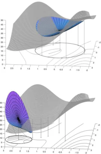
within the trust-region, and the resulting trial step accepted or rejected, depending on whether or not the achieved decrease in f sufficiently matches the predicted decrease in the model. The size of the trust-region is then reduced if the match is poor, or possibly enlarged if it is satisfactory. This broad algorithmic outline of course hides a number of prac-tical issues that are criprac-tical to good numerical per-formance. The most important is that the geometry of the sets Y(k) (i.e., the repartition the interpola-tion points y in Rn) must satisfy a condition called poisedness. If we consider a two-dimensional prob-lem, for instance, it is rather intuitive that the points in Y(k) should not all lie on a straight line. This poisedness condition can be formalized and tested [8, 9, 26] in various ways, but the key observation is that the same set of points cannot be used for ever as the algorithm proceeds, or even only modified to include the objective values at the new iterates. Fig-ure 1 illustrates the potentially desastrous effect on the model of a bad geometry (bottom), compared to a situation at a previous iteration where the geome-try is adequately poised (top).

As a consequence, it is necessary to improve the geometry of Y(k) at some iterations, typically by computing the objective function’s value at new points chosen to ensure sufficient poisedness.

How can we adapt this technique if we now as-sume that we know a partially separable decomposi-tion (2) of the objective? (We no longer assume that the matrices Ui are row subsets of the identity.) The answer, which is fully developed in [4], is based on a fairly obvious observation: instead of building m(k)_, a model of f in the neighbourhood of an iterate x(k), we may now build a collection of models {m(k)_i }q_i=1, where each m(k)_i now models fi in the same neigh-bourhood. Estimating a structured quadratic model of the form m(k)(x(k)+ s) = q X i=1 m(k)_i (x(k)+ s)

then requires at most (nmax+ 1)(nmax+ 2)/2 com-plete function evaluations, where we have defined nmax= maxi=1,...,qni. Since nmax  n, this is typi-cally order(s) of magnitude less that what is required for estimating an unstructured model. Moreover, nmaxis often independent of n.

Figure 1: How the evolution of the interpolation set can lead to a bad model when its geometry deteri-orates (the interpolation points are materialized by vertical bars from the surface to the plane, the model is quadratic and shown inside the trust-region)

However, we now have to manage q interpolation sets Y_i(k) (i = 1, . . . , q) over the iterations, instead of a single one. We then have to consider two possible cases: either it is possible for the user to evaluate a single element function fi(x) independently of the others (as we have assumed above), or the objective function must always be evaluated as a whole (i.e., only the collection of values {fi(x)}q_i=1 can be com-puted for a given x). In the second case, a straight-forward implementation of the algorithm could be very expensive in terms of function evaluations if one blindly applies a geometry improvement proce-dure to each Y_i(k). Indeed, computing a vector that

improves the geometry of the i-th interpolation set yields a vector having only ni “useful” components, and it is not clear which values should be assigned to the remaining n−nicomponents. The strategy in this case is to group the necessary individual func-tion evaluafunc-tions by applying the CPR procedure of Curtis, Powell and Reid [13] for estimating sparse Jacobian matrices to the n × q occurence matrix of variables xj into elements fi. (Other techniques in-volving graph colouring in the spirit of [1] are also possible). This typically results is subtantial savings in terms of function evaluations.

As in the previous section, we do not elaborate more on the algorithmic details and variants (and refer to [4] for this), but rather illustrate the po-tential benefits of the approach on a few examples. These benefits are already visible for medium-size problems, as is shown in Table 2 where the unstruc-tured algorithm (UDFO) is compared with its ver-sion using partially separable structure (PSDFO) on two CUTEr problems. The “I” version of PSDFO refers to the case where each element function fi is accessible, and the “G” version to the case where the complete collection of {fi(x)}qi=1 must be evaluated together for every x.

Problem n UDFO PSDFO(I) PSDFO(G)

ARWHEAD 10 311 30 54 15 790 30 56 20 1268 35 161 25 1478 37 198 BDQRTIC 10 519 348 358 15 1014 345 382 20 1610 509 596 25 2615 360 542

Table 2: Comparison of the number of function eval-uations required by DFO solvers for solving medium-size instances of problems ARWHEAD and BDQR-TIC(from [4]).

Again, the use of the partially separable struc-ture brings clear benefits, and these are also more pronounced when the values of the elements can be computed individually (case “I”). Table 3 indicates that these benefits extend to higher dimensions, as expected.

n GENHUMPS BROYDN3D

PSDFO(I) PSDFO(G) PSDFO(I) PSDFO(G)

10 114 168 53 70

20 200 345 56 84

50 202 357 68 114

100 249 433 153 342

200 253 436 123 278

Table 3: The number of function evaluations re-quired by PSDFO for solving problems GENHUMPS and BROYDN3D in various dimensions(from [4]).

5.

Interpolation

methods

for

sparse problems

We conclude our overview of the use of structure in derivative-free optimization by examining interpola-tion methods in the less favourable case where struc-ture is present but access to the individual values of the element functions fi(x) impossible. This may happen, for instance, when the objective function value results from a complicated simulation involv-ing a discretized partial differential equation (such as a complicated fluid calculation). In such cases, we often know that a partially separable decomposition of the form (2) exists (resulting, in our example, from the discretization topology), but we are only given the final value of f (x), without its decomposition in its element function values (note the difference with the “G” case in the previous section). This implies that we typically know that the Hessian of f , H(x), is sparse for every x, and know its structure. Can we exploit this (more limited) information?

As above, the idea is to construct a quadratic model m(k) that reflects the problem structure as much as possible: we thus need to construct a model whose Hessian has the same sparsity structure as that of the objective function. Interestingly, as noted in [2, 3], this is remarkably easy. Indeed, a given sparsity pattern is equivalent to a selection of a sub-set of the monomials generating the quadratic poly-nomials: if the (i, j)-th entry of H(x) (and thus the (j, i)-th one) is known to be zero for all values of x, this simply indicates that f can be modelled by a re-stricted quadratic polynomial that does not involve the monomial xixj. Thus the models m(k) may now be viewed as a linear combination of 1+n+nH mono-mials, where nH is the number of nonzeroes in the

lower triangular part of H(x). This last number is of-ten a small multiple of n, in which case the size of the interpolation set Y(k)_{is linear rather than quadratic} in n. The cost of evaluating a sparse quadratic model is thus also very attractive, although typically larger than that of a partially separable model (often in-dependent of n, as we have noted in the previous section).

These observations have been exploited in [2, 3], but also in [26] where Powell describes his successful UOBSQA code. The efficiency of this technique is attested by the results of Table 4, where the number of objective evaluations required for convergence is reported for UDFO (as in Table 2) and UOBSQA.

Problem Dimension UDFO UOBSQA UOBDQA

ARWHEAD n= 10 311 118 105 n= 15 790 170 164 n= 20 1268 225 260 n= 25 1478 296 277 BDQRTIC n= 10 519 350 288 n= 15 1014 594 385 n= 20 1610 855 534 n= 25 2615 1016 705

Table 4: Comparison of the number of function eval-uations required by UDFO, UOBSQA and UOB-DQA solvers for medium-size instances of problems ARWHEAD and BDQRTIC(from [4]).

Finally, one may argue that there is in fact no need that the sparsity structure of the model’s Hes-sian really reflects that of H(x). It is indeed possible to simply impose an a priori sparsity structure in or-der to reduce the size of the interpolation set, even if no sparsity information is available for H(x). This idea was suggested in [2] and implemented, in its ex-treme form where the model’s Hessian is assumed to be diagonal, in the UOBDQA code by Powell [25]. The excellent results obtained with this technique are also apparent in Table 4, even if one might guess that it will be mostly effective on problems whose Hessian is diagonally dominant. Potential extensions of this idea include the exploration of techniques (in-spired for instance from automatic learning) which adaptively taylor the imposed sparsity pattern to the effective behaviour of the objective function.

6.

Conclusions and perspectives

Given the discussion above, one may clearly conclude that yes, the derivative-free optimization algorithms can exploit problem structure to (sometimes dramat-ically) improve their efficiency. Moreover, the argu-ments presented also indicate that a richer structural information typically results in more substantial effi-ciency gains when using interpolation methods: the number of objective function evaluations necessary to estimate a quadratic model indeed ranges from quadratic in n (no structure) via linear in n (when exploiting sparsity) to independent of n (when using partially separability).

It is clear that the development of structure-aware derivative-free optimization methods and packages is only starting, and much remains to be done. We think, in particular, of extensions of the ideas dis-cussed here to the constrained case, and their appli-cations to neighbouring research areas, such as do-main decomposition (an ongoing project explores the use of partial separability in this context) and oth-ers. Developments in these directions combine both the more abstract aspects of algorithm design and theory with the very practical nature of a subject in high industrial demand. There is no doubt that they therefore constitute valuable research challenges.

Acknowlegment

Thanks to Luis N. Vicente for suggesting the topic of this note, and to Annick Sartenaer, the queen of referees, whose comments improved its form.

REFERENCES

[1] T. F. Coleman and J. J. Mor´e. Estimation of sparse Ja-cobian matrices and graph coloring problems. SIAM Journal on Numerical Analysis, 20:187–209, 1983. [2] B. Colson and Ph. L. Toint. Exploiting band structure

in unconstrained optimization without derivatives. Optimization and Engineering, 2:349–412, 2001. [3] B. Colson and Ph. L. Toint. A derivative-free

algo-rithm for sparse unconstrained optimization prob-lems. In A. H. Siddiqi and M. Koˇcvara, editors, Trends in Industrial and Applied Mathematics, pages 131–149, Dordrecht, The Netherlands, 2002. Kluwer Academic Publishers.

[4] B. Colson and Ph. L. Toint. Optimizing partially sep-arable functions without derivatives. Optimization Methods and Software, 20(4-5):493–508, 2005. [5] A. R. Conn, N. I. M. Gould, and Ph. L. Toint.

LANCELOT: a Fortran package for large-scale non-linear optimization (Release A). Number 17 in Springer Series in Computational Mathematics. Springer Verlag, Heidelberg, Berlin, New York, 1992. [6] A. R. Conn, N. I. M. Gould, and Ph. L. Toint. Trust-Region Methods. Number 01 in MPS-SIAM Series on Optimization. SIAM, Philadelphia, USA, 2000. [7] A. R. Conn, K. Scheinberg, and Ph. L. Toint. On the

convergence of derivative-free methods for uncon-strained optimization. In A. Iserles and M. Buh-mann, editors, Approximation Theory and Optimiza-tion: Tributes to M. J. D. Powell, pages 83–108, Cambridge, England, 1997. Cambridge University Press.

[8] A. R. Conn, K. Scheinberg, and Ph. L. Toint. Re-cent progress in unconstrained nonlinear optimiza-tion without derivatives. Mathematical Program-ming, Series B, 79(3):397–414, 1997.

[9] A. R. Conn, K. Scheinberg, and L. N. Vicente. Geometry of sample sets in derivative free optimization. Part I: polynomial interpolation. Technical Report 03-09, Departamento de Matem´atica, Universidade de Coimbra, Portugal, 2003. Revised September 2004. [10] A. R. Conn and Ph. L. Toint. An algorithm using

quadratic interpolation for unconstrained derivative free optimization. In G. Di Pillo and F. Gianessi, editors, Nonlinear Optimization and Applications, pages 27–47, New York, 1996. Plenum Publishing. Also available as Report 95/6, Dept of Mathemat-ics, FUNDP, Namur, Belgium.

[11] I. D. Coope and C. J. Price. On the convergence of grid-based methods for unconstrained optimization. SIAM Journal on Optimization, 11:859–869, 2001. [12] I. D. Coope and C. J. Price. Positive basis in

numer-ical optimization. Computational Optimization and Applications, 21, 2002.

[13] A. Curtis, M. J. D. Powell, and J. Reid. On the estima-tion of sparse Jacobian matrices. Journal of the In-stitute of Mathematics and its Applications, 13:117– 119, 1974.

[14] C. Davis. Theory of positive linear dependence. Ameri-can Journal of Mathematics, 76:733–746, 1954. [15] J. E. Dennis and V. Torczon. Direct search methods on

parallel machines. SIAM Journal on Optimization, 1(4):448–474, 1991.

[16] N. I. M. Gould, D. Orban, and Ph. L. Toint. CUTEr, a constrained and unconstrained testing environment, revisited. ACM Transactions on Mathematical Soft-ware, 29(4):373–394, 2003.

[17] A. Griewank and Ph. L. Toint. On the unconstrained optimization of partially separable functions. In M. J. D. Powell, editor, Nonlinear Optimization 1981, pages 301–312, London, 1982. Academic Press. [18] A. Griewank and Ph. L. Toint. Partitioned variable met-ric updates for large structured optimization prob-lems. Numerische Mathematik, 39:119–137, 1982. [19] A. Griewank and Ph. L. Toint. On the existence of

con-vex decomposition of partially separable functions. Mathematical Programming, 28:25–49, 1984. [20] R. Hooke and T. A. Jeeves. Direct search solution of

numerical and statistical problems. Journal of the ACM, 8:212–229, 1961.

[21] T. G. Kolda, R. M. Lewis, and V. Torczon. Optimization by direct search: new perspectives on some classical and modern methods. SIAM Review, 45(3):385–482, 2003.

[22] J. A. Nelder and R. Mead. A simplex method for func-tion minimizafunc-tion. Computer Journal, 7:308–313, 1965.

[23] M. J. D. Powell. A direct search optimization method that models the objective and constraint functions by linear interpolation. In S. Gomez and J. P. Hen-nart, editors, Advances in Optimization and Nu-merical Analysis, Proceedings of the Sixth Workshop on Optimization and Numerical Analysis, Oaxaca, Mexico, volume 275, pages 51–67, Dordrecht, The Netherlands, 1994. Kluwer Academic Publishers. [24] M. J. D. Powell. A direct search optimization method

that models the objective by quadratic interpola-tion. Presentation at the 5th Stockholm Optimiza-tion Days, Stockholm, 1994.

[25] M. J. D. Powell. On trust region methods for uncon-strained minimization without derivatives. Tech-nical Report NA2002/02, Department of Applied Mathematics and Theoretical Physics, Cambridge University, Cambridge, England, 2002.

[26] M. J. D. Powell. UOBYQA: unconstrained optimization by quadratic interpolation. Mathematical Program-ming, Series A, 92:555–582, 2002.

[27] C. J. Price, I. D. Coope, and D. Byatt. A convergent variant of the Nelder-Mead algorithm. Journal of Optimization Theory and Applications, 113(1):5–19, 2002.

[28] C. J. Price and Ph. L. Toint. Exploiting problem struc-ture in pattern-search methods for unconstrained op-timization. Optimization Methods and Software, (to appear), 2006.

[29] V. Torczon. On the convergence of the multidirectional search algorithm. SIAM Journal on Optimization, 1(1):123–145, 1991.

[30] D. Winfield. Function and functional optimization by interpolation in data tables. PhD thesis, Harvard University, Cambridge, USA, 1969.

[31] D. Winfield. Function minimization by interpolation in a data table. Journal of the Institute of Mathematics and its Applications, 12:339–347, 1973.