HAL Id: hal-00160809
https://hal.archives-ouvertes.fr/hal-00160809
Submitted on 8 Jul 2007
HAL is a multi-disciplinary open access
archive for the deposit and dissemination of
sci-entific research documents, whether they are
pub-lished or not. The documents may come from
teaching and research institutions in France or
abroad, or from public or private research centers.
L’archive ouverte pluridisciplinaire HAL, est
destinée au dépôt et à la diffusion de documents
scientifiques de niveau recherche, publiés ou non,
émanant des établissements d’enseignement et de
recherche français ou étrangers, des laboratoires
publics ou privés.
3-RPR parallel manipulators
Mazen Zein, Philippe Wenger, Damien Chablat
To cite this version:
Mazen Zein, Philippe Wenger, Damien Chablat. Singular curves and cusp points in the joint space of
3-RPR parallel manipulators. 2006, Orlando, United States. pp.1-6. �hal-00160809�
933
Abstract— This paper investigates the singular curves in
two-dimensional slices of the joint space of a family of planar parallel manipulators. It focuses on special points, referred to as cusp points, which may appear on these curves. Cusp points play an important role in the kinematic behavior of parallel manipulators since they make possible a nonsingular change of assembly mode. The purpose of this study is twofold. First, it reviews an important previous work, which, to the authors’ knowledge, has never been exploited yet. Second, it determines the cusp points in any two-dimensional slice of the joint space. First results show that the number of cusp points may vary from zero to eight. This work finds applications in both design and trajectory planning.
Keywords—Singular curves, cusp point, joint space, assembly
mode, 3-RPR parallel manipulator.
I. INTRODUCTION
Because at a singularity a parallel manipulator loses stiffness, it is of primary importance to be able to characterize these special configurations. This is, however, a very challenging task for a general parallel manipulator [1]. Planar parallel manipulators have received a lot of attention [1-8] because of their relative simplicity with respect to their spatial counterparts. Moreover, studying the formers may help understand the latters. Planar manipulators with three extensible leg rods, referred to as 3-RPR manipulators, have often been studied. Such manipulators may have up to six assembly modes [7]. The direct kinematics can be written in a polynomial of degree six [3]. Moreover, as is the case in most parallel manipulators, the singularities coincide with the set of configurations where two direct kinematic solutions coincide. It was first pointed out that to move from one assembly mode to another, the manipulator must cross a singularity [7]. But [8] showed, using numerical experiments, that this statement is not true in general. More precisely, this statement is true only under some special geometric conditions such as similar base and mobile platforms [9,10]. In fact, an analogous phenomenon exists in serial manipulators that can change their posture (inverse kinematic solution) without meeting a singularity in general, but not under special geometric simplification [8,11]. The nonsingular change of posture in serial manipulators was shown to be associated with the existence of points in the workspace where three inverse kinematic solutions meet, called cusp points [11]. Likewise, [9] pointed out that for a 3-RPR parallel manipulators (as well as
for its spatial counterpart, the octahedral manipulator), if a point with triple direct kinematic solutions exists in the joint space, then the nonsingular change of assembly mode is possible. A condition for three direct kinematic solutions to coincide was established. However, no systematic exploitation of this condition was possible because the algebra involved was too complicated and to the authors’ knowledge, the work of [9] has never been pursued yet.
In this paper, the abovementioned condition is reviewed and exploited. An algorithm for the systematic detection of cusp points is developed. It is shown that the number of cusp points depends on the slice of the joint space in which these cusp points are determined and the maximum number of cusp points depends on the geometry of the manipulator. This work helps better understand the topology of the joint space of parallel manipulators and finds applications in both design and trajectory planning.
The following section introduces the 3-RPR manipulator and its constraint equations. Sections III is devoted to the determination of the singular curves in slices of the joint space. The existence condition of cusp points is derived in section IV and an algorithm to automatically determine these points is briefly described. Section V is devoted to the explanation of the results obtained.
II. PRELIMINARIES
A. Manipulators Under Study
The manipulators under study are 3-DOF planar parallel manipulators with three extensible leg rods (Fig. 1).
x A1 A2 B2 B3 B1 θ L1 L2 2 d1 d3 d2 1 y A3 L3 3 H I
Figure 1. The 3-RPR parallel manipulator under study.
Singular curves and cusp points in the joint space of
3-RPR parallel manipulators
Mazen ZEIN , Philippe WENGER and Damien CHABLAT
Institut de Recherche en Communications et Cybernétique de Nantes UMR CNRS 6597 1, rue de la Noe, BP 92101, 44321 Nantes Cedex 03 France
This manipulator has been frequently studied [4-8]. Each of the three extensible leg rods is actuated with a prismatic joint. The geometric parameters of the manipulators are the three sides of the moving platform d1, d2, d3 and the position of the
base revolute joint centers defined by A1, A2 and A3. The
reference frame is centered at A1 and the x-axis passes through
A2. Thus, A1 = (0, 0), A2 = ( A2x , 0) and A3 = ( A3x , A3y).
B. Constraint Equations
Let L ≡ (L1, L2, L3) define the lengths of the three leg rods
and let θ ≡ (θ1, θ2, θ3) define the three angles between the leg
rods and the x-axis. The six parameters (L, θ) can be regarded as a configuration of the manipulator but only three of them are independent, so that the configuration space is a 3-dimensional manifold embedded in a 6-dimensional space. The dependency between (L, θ) can be identified by writing the fixed distances between the three vertices of the mobile platform B1, B2, B3,
which yield the following constraint equations
[
] [
]
[
] [
]
[
] [
]
2 1 2 1 2 1 1 2 2 3 2 3 2 2 2 3 1 3 1 3 3 ( , ) ( , ) ( , ) ( , ) ( , ) 0 ( , ) ( , ) ( , ) ( , ) ( , ) 0 ( , ) ( , ) ( , ) ( , ) 0( , )
T T T d d d ⎧ Γ = − − − = ⎪⎪Γ = − − − = ⎨ ⎪ Γ = − − − = ⎪⎩ L θ b L θ b L θ b L θ b L θ L θ b L θ b L θ b L θ b L θ L θ b L θ b L θ b L θ b L θ (1)where bi is the vector defining the coordinates of Bi in the
reference frame as function of L and θ. For more simplicity, (L, θ) will be omitted in the following equations.
Expanding each Γi as a series about the configuration (L, θ)
yields 3 3 1 1 2 3 3 1 1 3 3 1 1 2 .. 0
1
...
!
1
!
i i i i j j j j i i i j j j j n i i i j j j j L L L L L Ln
θ θ θ θ θ θ = = = = = = ⎛ ∂ ∂ ⎞ ΔΓ =⎜⎜ Δ + Δ ⎟⎟Γ + ∂ ∂ ⎝ ⎠ ⎛ ∂ ∂ ⎞ Δ + Δ Γ ⎜ ⎟ ⎜ ∂ ∂ ⎟ ⎝ ⎠ ⎛ ∂ ∂ ⎞ Δ + Δ Γ + = ⎜ ⎟ ⎜ ∂ ∂ ⎟ ⎝ ⎠+ +
∑
∑
∑
∑
∑
∑
(2)If one keeps only the first-order and second-order terms, Eq. (2) can be written in matrix form as follows
2 2 2 1 1 1 2 2 2 2 2 2 2 2 2 2 2 2 2 3 3 3 2 2 1 1 0 2 2 T T T T T T T T T ∂ ∂ Δ = Δ + Δ ∂ ∂ ⎡ ∂ Γ ⎤ ⎡Δ ∂ Γ Δ ⎤ Δ Δ ⎡Δ ∂ Γ Δ ⎤ ⎢ ⎥ ⎢ ∂ ⎥ ∂ ∂ ⎢ ∂ ⎥ ⎢ ⎥ ⎢ ⎥ ⎢ ⎥ ⎢ ⎥ ∂ Γ ∂ Γ ∂ Γ ⎢ ⎥ ⎢ ⎥ + ⎢Δ Δ + Δ⎥ ⎢ Δ ⎥+ ⎢Δ Δ ⎥= ∂ ⎢ ∂ ∂ ⎥ ∂ ⎢ ⎥ ⎢ ⎥ ⎢ ⎥ ∂ Γ ∂ Γ ⎢Δ Δ ⎥ ⎢Δ ∂ Γ Δ ⎥ ⎢Δ Δ ⎥ ⎢ ∂ ⎥ ∂ ∂ ⎢ ∂ ⎥ ⎣ ⎦ ⎢⎣ ⎥⎦ ⎣ ⎦ Γ Γ Γ θ L θ L θ L θ θ θ L L L θ L θ θ θ L L L θ θ L L θ θ θ L L L θ θ L L (3) Equation (3) can be used to describe an arbitrary local motion at a given configuration of the manipulator [9]. When first order terms of Eq. (3) are sufficient to describe the motion, the manipulator is in a regular configuration and the following equation can be used instead of Eq. (3)
(
,)
(
,)
0 ∂ ∂ Δ + Δ = ∂ ∂ Γ L θ Γ L θ θ L θ L (4)Otherwise the configuration (L, θ) is special and the manipulator meets a singularity. This happens when the constraint Jacobian ∂ ∂Γ/ θ drops rank so that the second order terms of the equation (3) are needed to describe the constraints. The three vertices of the moving platform have the following coordinates in the fixed reference frame
( )
( )
( )
( )
( )
( )
1 1 1 1 1 2 2 2 2 2 2 3 3 3 3 3 3 3 cos sin cos sin cos sin . T T x T x y L L A L L A L A L θ θ θ θ θ θ = ⎡⎣ ⎤⎦ =⎡⎣ + ⎤⎦ ⎡ ⎤ =⎣ + + ⎦ b b bThus, the constraint Jacobian can be put in the following form
(
)
(
)
(
)
(
)
1 2 1 2 12 2 1 21 2 2 2 2 3 2 3 2 3 3 3 23 3 2 2 23 3 3 1 3 1 3 31 3 3 3 1 31 3 1 3 3 0 ( ) ( ) 2 0 ( ( 0 ) ) x x x x x x y y x x y y L A s L s L L s A s L A A s L A A s L s A c L s A c L A s L s L A s L s A c A c ⎡ ⎤ ⎢ + − ⎥ ⎢ ⎥ ⎢ ⎥ − − − ⎢ ⎥ ∂ = ⎢ ⎥ ∂ ⎢ − + − + ⎥ ⎢ ⎥ − − − ⎢ ⎥ ⎢ − − ⎥ ⎢ ⎥ ⎣ ⎦ Γ θ (5)where si =sin
( )
θi , ci =cos( )
θi and sij =sin(
θ θi− j)
. III. SINGULAR CURVES IN 2-DIMENSIONAL SLICES OF THECONFIGURATION SPACE
The singularities were determined in [9] by looking for the configurations where det(∂ ∂Γ/ θ) but this equation was
incorrectly displayed. To derive the right equation, we have used a geometric approach that is much more direct than the calculation of the determinant, which does not simplify easily. The manipulator is in a singular configuration whenever the axes of its three leg rods intersect (possibly at infinity). The derivation of this geometric condition is straightforward and yields the following equation
(
)
2x 2 31 3x 3 3y 3 12 0,
A s s + A s −A c s = (6)
which we have checked successfully with several manipulator geometries. In order to reduce the dimension of the problem, [9] shows that it is possible to consider two-dimensional slices of the configuration space by fixing one of the leg rod lengths. By doing so, only two parameters are needed to fully define a configuration. For a fixed value of L1, a configuration may be
fully defined by either (α,θ1) or (L2, L3). Note that in the first
case, the configuration is defined in the output space by the position and the orientation of the moving platform (L1 and θ1
define the position of B1 in the plane and α defines the
orientation of the moving platform in the plane). In the second case, the configuration is defined in the joint space by the three
leg rod lengths.
Now, for any fixed value of L1, it is possible to plot the
singular curves in either (α,θ1) or (L2, L3). But we first need to
rewrite Eq. (6) as function of L1, α and θ1, which we do with
the help of the following set of geometric equations
( )
( )
(
)
(
)
2 2 2 1 1 1 2 2 1 1 1 3 3 3 1 1 3 3 3 3 1 1 3 c c cos 0 s s sin 0 c c cos 0 s s sin 0, x x y A L L b L L b A L L b A L L b α α α β α β + − − = ⎧ ⎪ − − = ⎪ ⎨ + − − + = ⎪ ⎪ + − − + = ⎩ (7)where β is the (fixed) angle between B1B2 and B1B3 (Fig. 1).
The first (resp. last) two equations make it possible to express L2 (resp. L3) as function of L1, α and θ1. Then, c2 and s2 (resp.
c3 and s3) are calculated as function of L1, α and θ1 from the
first (resp. last) two equations of (7) and their expressions are input in Eq. (6), which, now, depend only on L1, α and θ1. The
resulting equation makes it possible to plot the singular curves directly in (α, θ1). To get the curves in (L2, L3), we use the
expressions of L2 and L3 as function of L1, α and θ1.
Figure 2 shows the singular curves obtained for the 3-RPR manipulator of [8, 9]. The geometric parameters of this manipulator are recalled below in an arbitrary length unit:
A1=(0, 0) d1=17.04
A2=(15.91, 0) d2=16.54
A3=(0, 10) d3=20.84
L
2L
3Figure 2. Singular curves in (L2,L3) for L1=14.98. Number of assembly modes is displayed in each region.
The singular curves were plotted in the slice of the joint space defined by L1=14.98 as in [9]. These curves give rise to
several regions with a constant number of assembly modes in each region. Figure 2 shows that several cusp points exist where three assembly modes coalesce. In [9] the number of cusp points was claimed to be five. It will be shown in next section that a sixth cusp point does exist.
IV. DETERMINATION OF THE CUSP POINTS
For serial 3-DOF manipulators, the cusp points can be determined by deriving the condition under which the inverse kinematics polynomial admits three identical roots [11]. However this approach is intractable when applied to the direct kinematics polynomial of 3-RPR manipulators because the algebra involved is too complicated.
An interesting alternative approach was proposed in [9] by writing the condition under which the manipulator loses first and second order constraints. The resulting condition for triple coalescence of assembly modes was shown to take the following form 2 2 2 1 2 3 1 2 2 2 3 2 0, T⎡u ∂ Γ +u ∂ Γ +u ∂ Γ ⎤ = ⎢ ∂ ∂ ∂ ⎥ ⎣ ⎦ v v θ θ θ (8)
where vis a unit vector in the right kernel of matrix ∂ ∂Γ/ θ , and u1, u2, u3 are the three components of the unit vector uthat
spans the left kernel. Vectors uand vcan be chosen in the set of nonzero rows and columns of the adjoint of matrix
∂ ∂Γ/ θ (i.e. the matrix of cofactors of the transpose of ∂ ∂Γ/ θ ),
respectively.
Calculating the adjoint of ∂ ∂Γ/ θ from Eq. (5) yields
adj 1 2 2 5 3 5 3 4 2 6 3 6 1 4 4 5 1 6 k k k k k k k k k k k k k k k k k k − ⎛ ⎞ ∂ ⎛ ⎞ ⎜= ⎟ ⎜∂ ⎟ ⎜ ⎟ ⎝ ⎠ ⎜− ⎟ ⎝ ⎠ Γ θ (9)
Expressions for k1 through k6 were reported in [9] with
several errors. The corrected expressions are given below:
(
)
(
)
(
)
(
)
(
)
(
)
(
)
(
)
1 2 3 2 2 3 23 3 2 2 3 1 13 3 3 3 3 3 3 3 2 3 2 23 3 3 4 1 3 13 3 1 3 1 5 2 1 12 2 2 6 1 2 12 2 1 2 2 2 2 2 2 x x y x y x x y x y x x k L A A s L s A c k L L s A s A c k L A A s L s A c k L L s A s A c k L L s A s k L L s A s = − + − = − + − = − − + − = + − = − + = + (10)Taking u (resp. v) as the first row (resp. column) of (9), Eq. (8) can be written as
(
)
2 1 2 2 2 3 1 2 1 2 3 4 1 4 1 2 2 2 5 2 3 5 2 3 4 1 4 0 k k k k k k k k k k k k k k k k k k ⎛ ⎞ ⎛ ∂ Γ ∂ Γ ∂ Γ ⎜⎞ ⎟ − ⎜ − + ⎟⎜ ⎟= ∂ ∂ ∂ ⎝ θ θ θ ⎠⎜⎝− ⎟⎠ (11) where(
)
(
)
(
)
(
)
(
)
2 1 2 1 2 21 1 2 21 1 1 2 21 2 2 2 1 21 2 2 2 2 3 2 2 2 3 23 2 3 23 3 2 3 2 3 3 2 3 23 2 23 3 3 2 1 3 1 3 31 3 1 1 3 3 2 0 2 0 0 0 0 0 0 0 ( ) 2 0 ( ) 0 0 2 x x x x y x x y x y L A c L c L L c L L c L A c L c L A A c L L c L c A s L A A c L L c L c A s L A c L c A s L L + − ⎡ ⎤ ∂ Γ ⎢ ⎥ = − − − ∂ ⎢⎣ ⎥⎦ ⎡ ⎤ ⎢ ⎥ ⎢ ⎥ − − ⎢ ⎥ ∂ Γ = ⎢ − ⎥ − − ∂ ⎢ ⎥ ⎢ − ⎥ ⎢ − ⎥ + − ⎢ ⎥ ⎣ ⎦ + + − ∂ Γ = ∂ θ θ θ(
)
31 1 3 31 3 1 31 3 3 3 3 0 0 0 0 x y c L L c L L c A c A s ⎡ ⎤ ⎢ ⎥ ⎢ ⎥ − − − ⎢ ⎥ ⎣ ⎦ (12)In [9], Eq. (11) was left as such and no information was provided on how to use it in a computer program. We have developed an algorithm to solve this equation for any 3-RPR manipulator and we have implemented it in Maple. The resulting Maple program is available on our webpage (because of the anonymous review process, the url cannot be displayed in this proposal). Equation (11) is first expressed as function of L1, α and θ1, which we do as in section III using Eqs. (7).
Then, sin(θ1), cos(θ1), sin(α) and cos(α) are replaced by their
expression in t1 = tan(θ1/2) and t = tan(α/2), respectively, in
order to have pure algebraic expressions for Eqs. (6) and (11). At this stage, Eq. (6) (resp. Eq. (11)) results in a 4th-order (resp. 12th-order) polynomial in tandt1. Then, t is eliminated
from these two polynomials by computing their resultant [12]. Because Eq. (11) is complicated, this task requires careful preliminary algebraic manipulation. The resulting equation has the following general form
3 1 1 2 1 2 3 ... 1 0 n n a a a a a n n P P P P −P Q − = (13)
where Q is a 24th-order univariate polynomial in t1 and P1,
P2,…,Pn are quadratic and quartic polynomials in t1. It is well
known that elimination often generate spurious solutions [12]. This is the case in Eq. (13) where P1, P2,…,Pn can be shown to
define no cusp points. Thus, only the 24th-order univariate polynomial Q is relevant. Once the real roots of Q are calculated, t can be found by back-substitution in Eq. (6) and solving for the resulting quartic equation. Finally, the cusps points are obtained using the expressions of L2 and L3 as
function of L1, α and θ1.
The algorithm was first run for the manipulator studied in the previous section and for L1=14.98 (Fig. 2). Six cusp points
were identified instead of five [9]. These points are pinpointed with circles in Fig. 3. The sixth point missed in [9] is circled with bold lines and in-boxed in a separate view. As reported in [9], the points appearing on L2=0 and L3=0 are not cusp points
because the constraint equations are non-differentiable.
L
2L
3Figure 3. Singular curves in (L2,L3) for L1=14.98. The six cusp points are circled, the one in-boxed in a separate view was missed in [9].
V. DESCRIPTIVE ANALYSIS
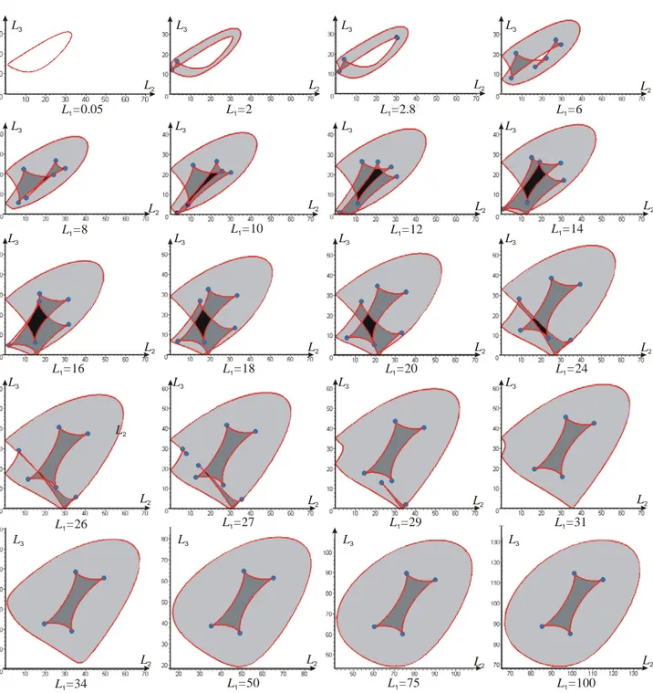
In this section the singular curves are analysed in several slices of the joint space for the manipulator of [8, 9] whose geometric parameters were given in section III. Figure 4 depicts the singular curves for increasing values of L1 and
shows that the number of cusp points is not the same for all slices as we may have 0, 2, 4, 6 or 8 cusp points. In Fig. 4, regions with two assembly modes (resp. four, six) are filled in light grey (resp. in dark grey, in black). Zero-cusp slices are obtained for very small values of L1 only (L1=0.05 in Fig. 4),
where the singular curves are made of two separate closed curves that define only one small region with two assembly modes and a large void (note, the two curves are so close that the region cannot be seen on Fig. 4). When L1 is increased two
cusp points appear, the void gets smaller and a four-solution region appears (L1=2). Then two more cusp points appear,
defining one more four-solution region (L1=2.8). We have six
cusp points and a small void at L1=6; for L1=8, 10, 12, 14, 16,
18, 20, 24 and 26, we have always six cusp points but the void is replaced with a six-solution region. Eight cusp points were found in a small vicinity of L1=27. Then two cusp points and
the six-solution region disappear (L1=29). Finally, the number
of cusp points stabilizes to four, defining one central four-solution region surrounded by a two-four-solution region (L1=31,
…). Interestingly, this last pattern is very similar to the one often observed in a cross-section of the workspace of 3-R serial manipulators [13]. However, serial manipulators feature the same pattern in all cross-sections (the sections which passes through the first revolute joint axis), and variation in the number of cusp points arises only from a modification of the manipulator geometry.
The above analysis shows that the joint space topology of 3-RPR manipulators is very complicated. Contrary to serial manipulators, the shape of the singular curves and the number of cusps points depend on which slice is chosen in the joint space. Thus, planning trajectories is not easy. However, we have noticed that the pattern stabilizes for sufficiently large values of L1.
L2 L1=34 L2 L1=50 L1=75 L2 L2 L3 L3 L3 L3 L1=100 L2 L2 L2 L2 L2 L3 L3 L3 L3 L1=27 L1=29 L1=31 L1=26 L2 L2 L2 L1=16 L1=18 L1=20 L1=24 L2 L3 L3 L3 L3 L2 L1=8 L1=10 L2 L2 L1=12 L2 L3 L3 L3 L3 L1=14 L2 L1=0.05 L2 L1=2 L2 L2 L1=6 L3 L3 L3 L3 L1=2.8
Figure 4. Singular curve patterns for increasing values of L1.
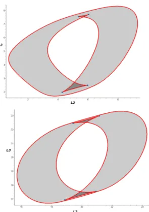
This feature has been observed in many other manipulator geometries. For example, the 3-RPR manipulator defined by the following geometric parameters
A1=(0., 0.) d1=1.3
A2=(3, 0.) d2=0.9
A3=(1.1, 2.7) d3=0.4
has a constant pattern as soon as L1>5 (Fig. 5). Note that, in
contrast with the stabilized pattern obtained for the preceding manipulator, this one features a large void.
Most research on parallel manipulators has been focused on the analysis and optimization of the workspace. If the
workspace is useful for manipulator design, the analysis of singular curve patterns in the joint space can be used as a complementary tool to compare several manipulator geometries.
Figure 5. Stabilized singular curve pattern for another manipulator geometry plotted for L1=5 (up) and L1=20 (down).
VI. CONCLUSIONS
A descriptive analysis of the singular curves in slices of the joint space of 3-RPR parallel manipulators was conducted in this paper, with a special focus on the determination of cusp points on these singular curves. This work was based on a meticulous review of a previous theoretical work and the recalculation of some of its formulas that were not correctly displayed. The existence condition of triple assembly modes was exploited and an algorithm for the automatic detection of cusp points was developed and run for several manipulators with arbitrary geometries. It was shown that contrary to what arises in serial manipulators where any cross section of the workspace exhibits the same pattern of singular curves and cusp points, this pattern depends on the choice of the slice in the joint space for a given 3-RPR parallel manipulator. On the
other hand, we have noticed that it is possible to have a constant pattern by adjusting the joint limits. It has been observed that the maximum number of cusps depends on the manipulator geometry but no manipulators were found with more than eight cusp points. Most research on parallel manipulators has been focused on the analysis and optimization of the workspace. This work is a complementary tool that helps better understand the topology of the joint space of parallel manipulators and finds applications in both design and trajectory planning.
VII. REFERENCES [1] J-P. Merlet, Parallel Robots, Kluwer Academics, 2000.
[2] C. Gosselin, and J. Angeles, “Singularity analysis of closed loop kinematic chains,” IEEE Transactions on Robotics and Automation, vol. 6, no. 3, 1990. [3] C. Gosselin, J. Sefrioui, and M.J. Richard, “Solution polynomiale au problème de la cinématique directe des manipulateurs parallèles plans à 3 degrés de liberté,” Mechanism and Machine Theory, vol. 27, no. 2, pp. 107-119, 1992.
[4] J. Sefrioui, and C. Gosselin, “On the quadratic nature of the singularity curves of planar three-degree-of-freedom parallel manipulators,” Mechanism
and Machine Theory, vol. 30, no. 4, pp. 535-551, 1995.
[5] P. Wenger, and D. Chablat, “Definition sets for the direct kinematics of parallel manipulators,” 8th Conference on Advanced Robotics, pp. 859-864,
1997.
[6] I. Bonev, D. Zlatanov, and C. Gosselin, “Singularity Analysis of 3-DOF Planar Parallel Mechanisms via Screw Theory,” ASME Journal of Mechanical
Design, vol. 125, no. 3, pp. 573–581, 2003.
[7] K.H. Hunt, and E.J.F. Primrose, “Assembly configurations of some In-parallel-actuated manipulators,” Mechanism and Machine Theory, vol. 28, no. 1, pp.31-42, 1993.
[8] C. Innocenti, and V. Parenti-Castelli, “Singularity-free evolution from one configuration to another in serial and fully-parallel manipulators. Journal of
Mechanical design. 120. 1998.
[9] P.R. Mcaree, and R.W. Daniel, “An explanation of never-special assembly changing motions for 3-3 parallel manipulators,” The International Journal of
Robotics Research, vol. 18, no. 6, pp. 556-574. 1999.
[10] Xianwen Kong and Clément M. Gosselin, “Forward displacement analysis of third-class analytic 3-RPR planar parallel manipulators,” Mechanism and
Machine Theory, Vol. 36, No. 9, pp. 1009--1018.
[11] J. El Omri and P. Wenger: “How to recognize simply a non-singular posture changing 3-DOF manipulator,” Proc. 7th Int. Conf. on Advanced
Robotics, p. 215-222, 1995.
[12] B. Buchberger, G. E Collins and R. Loos: “Computer Algebra: Symbolic & Algebraic Computation,” Springer-Verlag, Wien, pp. 115-138, 1982. [13] M. Baili, P. Wenger and D. Chablat, “A classification of 3R orthogonal manipulators by the topology of their workspace,” IEEE Int. Conf. on Robotics

![Figure 2 shows the singular curves obtained for the 3-RPR manipulator of [8, 9]. The geometric parameters of this manipulator are recalled below in an arbitrary length unit:](https://thumb-eu.123doks.com/thumbv2/123doknet/11588530.298562/4.892.115.397.576.954/singular-obtained-manipulator-geometric-parameters-manipulator-recalled-arbitrary.webp)
![Figure 3. Singular curves in (L 2 ,L 3 ) for L 1 =14.98. The six cusp points are circled, the one in-boxed in a separate view was missed in [9]](https://thumb-eu.123doks.com/thumbv2/123doknet/11588530.298562/5.892.471.813.121.398/figure-singular-curves-points-circled-boxed-separate-missed.webp)