HAL Id: hal-01154714
https://hal-ensta-paris.archives-ouvertes.fr//hal-01154714
Submitted on 22 May 2015HAL is a multi-disciplinary open access
archive for the deposit and dissemination of sci-entific research documents, whether they are pub-lished or not. The documents may come from teaching and research institutions in France or abroad, or from public or private research centers.
L’archive ouverte pluridisciplinaire HAL, est destinée au dépôt et à la diffusion de documents scientifiques de niveau recherche, publiés ou non, émanant des établissements d’enseignement et de recherche français ou étrangers, des laboratoires publics ou privés.
Complicated dynamics exhibited by thin shells
displaying numerous internal resonances: application to
the steelpan
Mélodie Monteil, Cyril Touzé, Olivier Thomas
To cite this version:
Mélodie Monteil, Cyril Touzé, Olivier Thomas. Complicated dynamics exhibited by thin shells dis-playing numerous internal resonances: application to the steelpan. International Congress on Sound and Vibration ICSV 19, Jul 2012, Vilnius, Lithuania. �hal-01154714�
SHELLS DISPLAYING NUMEROUS INTERNAL
RESO-NANCES : APPLICATION TO THE STEELPAN
M´elodie Monteil, Cyril Touz´e
UME ENSTA-Paristech, PALAISEAU, France
Olivier Thomas
LMSSC CNAM, PARIS, France
Nonlinear vibrations of a steelpan are experimentally studied. Modal analysis reveals the existence of numerous modes displaying internal resonances of order two and three, enabling the structure to transfer energy from low or high frequency modes. The com-plicated dynamics in forced vibrations is precisely measured by following the different harmonics of the responses. Energy transfers are explained in light of high order cou-plings, and a simple model displaying 1:2:2 internal resonance is fitted to the experiments. The measurements reveals that mode couplings are activated for very low amplitudes of order 1/25 times the thickness, and that numerous modes are rapidly excited, giving rise to complex shape frequency response functions. This ease in transferring energy and coupling modes is a key feature for explaining the peculiar tone of the steelpan.
1.
Introduction
Steelpans are a tuned percussion instruments family coming from Trinidad and Tobago. They are made of oil barrels that are subjected to several stages of metal forming that stretch and bend the structure. The top of the barrel is pressed, hammered, punched and burnt in order to obtain a sort of main bowl within which convex substructures are formed. Each convex dome corresponds to a musical note, which natural frequency is precisely tuned according to harmonic relationships.
Depending on the instrument, on the selected note as well as on the tuner know-how, different harmonic relationships may be observed. In all cases, the second mode is tuned to twice the frequency of the fundamental, giving rise to 1:2 relationship. Due to the localization [2] it is generally observed that the second mode is degenerate so that a 1:2:2 internal resonance is present. The third mode is tuned either at the third or at the fourth of the fundamental frequency, so that 1:2:2:3 or 1:2:2:4 internal resonances are possible. Finally, higher modes are also found to be tuned, hence the presence of modes at six times and/or eight times the fundamental frequency, are also generally found [4, 2].
In normal playing where a note is stroke with a stick, vibrations amplitudes are such that geometric nonlinearities cannot be neglected, and is recognized as a key feature for explaining
19th
International Congress on Sound and Vibration, Vilnius, Lithuania, July 8–12, 2012
the peculiar tone of the steelpan [1]. This nonlinearity combined with the numerous possible internal resonances, activates energy transfer to higher modes. In playing conditions, energy transfers up to a dozen of mode are usually observes.
The aim of this work is to study energy exchanges and activation of internal resonances in the nonlinear dynamics exhibited by the steelpan. Forced vibrations and frequency response curves are used to identify and localize instabilities and mode coupling. For that purpose, the different harmonics of the responses are followed during controlled step-by-step, forward and backward sweeps around the resonance of the first and the second eigenfrequencies. Frequency-response functions (FRFs) show complicated dynamics and activation of mode coupling from low to high-frequency. Scenarii of energy transfers are assumed, and checked versus comparisons of analytical FRFs obtained from multiple scale analysis of systems displaying 1:2:2 internal resonance. The study reveals that mode couplings are excited for vibration amplitude as small as 1/25 the thickness, as well as the fact that numerous modes are involved in the vibration for a medium amplitude range of vibration.
2.
Measurements
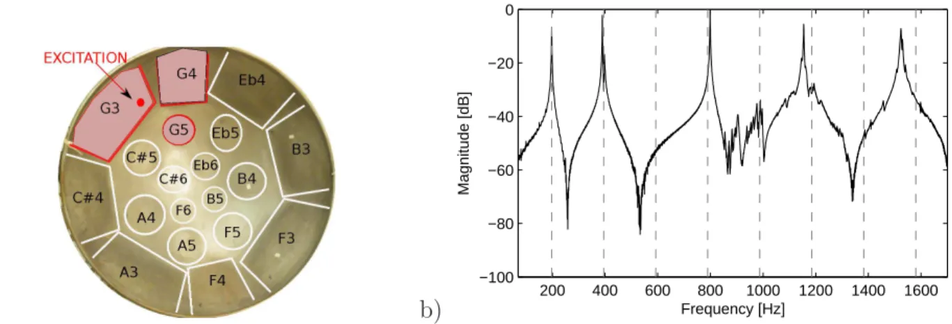
The steelpan shown in figure 1(a) is a right barrel of a double second (middle-high fre-quency steelpan). It is composed of 19 precisely tuned notes, distributed on three concentric circles, the lower notes being on the outer circle. This study is more particularly focused on G3 (of fundamental frequency f1) and its harmonically tuned neighbours G4 (2f1) and G5 (4f1).
2.1 Modal analysis and linear characterization
Modal analysis is used to characterize the linear behaviour of the structure by identifying eigenfrequencies, mode shapes and modal damping coefficients. In the experiment, the steelpan is excited by a homemade non-contact coil/magnet exciter, for which the equivalent point force is estimate by recording the current intensity in the coil [5]. The steelpan vibratory response, in velocity, is measured with a laser vibrometer. Figure 1 shows the precise location of the excitation point E on the G3 note, and the measured transfer function in the frequency range [0, 1700] Hz. One can see that the first three modes are perfectly tuned like f1, 2f1 and 4f1,
while the fourth and the fifth departs a little from the perfect harmonic relationship, and are slighlty shifted from the exact 6f1 and 8f1 relation. At 2f1, a double peak is clearly visible
indicating that the mode is degenerate with two mode shapes around the same frequency.
a) b) 200 400 600 800 1000 1200 1400 1600 −100 −80 −60 −40 −20 0 Magnitude [dB] Frequency [Hz]
Figure 1. a) Modal analysis of the steelpan excited on the note G3. b) Associated frequency response function, measured at the excitation point E
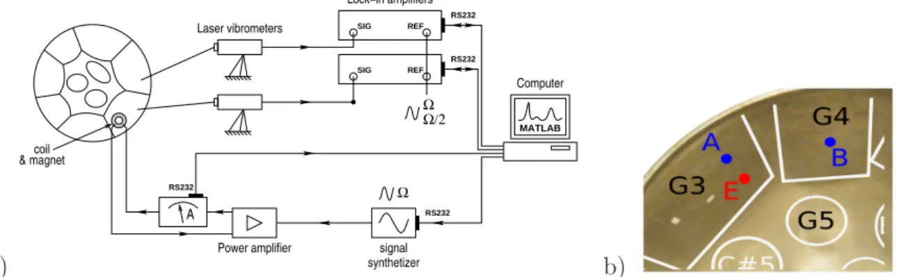
The experimental set-up used for measuring FRFs is shown in figure 2(a), as well as the location of two selected measurement points, the first one (A) on the G3 note, the second one (B) on the G4 note (Fig. 2(b)). In the remainder of the paper, w(x, t) denote the transverse displacement, and wA, wB refer to the displacement at points A and B, respectively. Linear
measurements are performed by selecting a very small value of the excitation force.
a) coil & magnet A Laser vibrometers Lock−in amplifiers
Power amplifier signal synthetizer RS232 SIG REF Ω/2 Ω Computer MATLAB Ω RS232 RS232 SIG REF RS232 b)
Figure 2. a) Experimental set-up. b) Location of points measurements on the steelpan’s notes
Forward and backward frequency sweeps around the linear resonances are then measured and reported in figure 3. Selecting the excitation frequency fdr is in the vicinity of f1 allows a
precize measurement of the fundamental frequency at f1=197.6 Hz (Fig. 3(a)). The associated
mode shape is, as awaited, located on the note G3 with a single maximum, as shown in fig-ure 3(d). When fdr ≃ 2f1, two degenerate modes are identified. The first one (denoted mode
2) has for eigenfrequency f2=390 Hz and its mode shape is composed of the second vibration
pattern of the G3 note together with the fundamental vibration mode of the G4 note. The sec-ond one (denoted mode 3) has its eigenfrequency at f3=397.8 Hz and its mode shape is similar
except the fact that the pattern on the G4 note is out of phase (Fig. 3(b), 3(e), 3(f)). Finally, using the measurement at point B instead of the one at point E used for the transfer function in figure 1(b) reveals that at 4f1, two degenerate modes are also at hand, with eigenfrequencies
f4=789.5 Hz and f5=799.3 Hz (Fig. 3), and mode shapes as shown in figure 3(g) and 3(h).
This linear analysis shows that almost harmonic relationships are present and the occur-rence of 1:2:2:4:4 internal resonance is possible. More complicated scenarii invoking also the presence of the modes at 6f1and 8f1 may also be activated in certain vibratory regimes. Forced
vibrations at higher force amplitudes will now be detailed to depict how energy is transferred between these modes.
2.2 Nonlinear dynamics of the steelpan forced vibrations
In order to study the nonlinear behaviour of the steelpan, the amplitude of the excitation is increased. Two cases are investigated, where the driving frequency fdris selected either at the
fundamental frequency, or in the vicinity of the second mode. The measured vibration obtained from the laser vibrometer at point A is decomposed in harmonic components (fdr, 2fdr, 3fdr,
...) by means of a lock-in amplifier (Fig. 2a). Frequency response curves are obtained by a step-by-step increasing and decreasing frequency sweep, where for each point, a settle time is awaited for the transient to die away, then fourty measurement amplitudes are recorded in the steady state (Poincar´e stroboscopy), in order to discriminate periodic and quasi-periodic regimes. Measurement of a foward sweep with the selected frequency range lasts 2 hours.
19th
International Congress on Sound and Vibration, Vilnius, Lithuania, July 8–12, 2012
a) 192 194 196 198 200 202 0 2 4 6 x 10⁻⁴ wA [mm] fdr [Hz] d) mode 1 : 197.6 Hz b) 385 390 395 400 0 2 4 6 x 10⁻⁴ wA [mm] f dr [Hz] e) f) mode 2 : 390 Hz mode 3 : 397.8 Hz c) 770 780 790 800 0 1 2 x 10⁻⁵ wB [mm] f dr [Hz] g) h) mode 4 : 789.5 Hz mode 5 : 799.3 Hz
Figure 3. Displacement measurements for a low amplitude forced excitation (I=0.01A) and associated mode shapes around f1 (– –) ; 2f1 (– · –) and 4f1 (· · · ·)
2.2.1 Low frequency excitation (fdr ≃ f1)
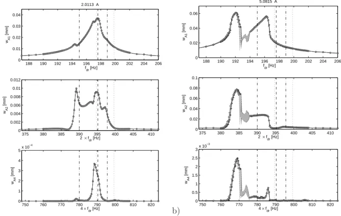
Two levels of excitation (I=2A and I=5A) are shown in figure 4 to investigate the nonlin-ear dynamics of the steelpan in the vicinity of the first eigenfrequency at 197.6 Hz. Harmonics 1, 2 and 4 of the recorded displacement are shown, they are denoted respectively by wA1, wA2
and wA4.
For the first excitation amplitude shown (I=2A), the coupling between the first three modes is evident, as well as with the fourth mode at 789.5 Hz. Markers are inserted into the figures to precisely locate, in frequency, the different eigenfrequencies of the system. The complex shape of wA2 highlights the fact that the 1:2:2 internal resonance is already activated with a strong
transfer of energy from the first to the second and third modes. Interestingly, this coupling is already effective for a vibration amplitude of the fundamental of 0.04 mm. As the thickness is 1 mm, one can conclude that the geometric nonlinearities effect are noticeable in the system response for vibration amplitudes of 1/25 times the thickness. Finally, wA4 participate to the
response with a non-negligible amplitude which is not slaved to wA2, with a strong peak in
the vicinity of the fourth mode at 789.5 Hz. On the other hand, the second configuration at 799.3 Hz do not appear in the response so that one can assume that a 1:2:2:4 resonance is here activated.
For the second vibration amplitude (I=5A), the same resonance scenario seems to be at work, but the dynamics is now complicated with the appearance of a quasiperiodic regime in a fre-quency range around 193 Hz and with a slight difference between increasing and decreasing frequency experiments. The shape of the solution branches, as compared to theoretical ones of the 1:2 and 1:2:2 internal resonance that can be found in [3, 2], appears slightly different, as a reflection of the fact that the cubic nonlinearity is not anymore negligible. Howerver, the 1:2
a) 188 190 192 194 196 198 200 202 204 206 0 0.01 0.02 0.03 0.04 wA1 [mm] f dr [Hz] 2.0113 A 375 380 385 390 395 400 405 410 0 0.002 0.004 0.006 0.008 0.01 0.012 wA2 [mm] 2 × f dr [Hz] 750 760 770 780 790 800 810 820 0 1 2 3 4 5x 10 −4 wA4 [mm] 4 × f dr [Hz] b) 188 190 192 194 196 198 200 202 204 206 0 0.02 0.04 0.06 wA1 [mm] fdr [Hz] 5.0815 A 375 380 385 390 395 400 405 410 0 0.02 0.04 0.06 0.08 0.1 wA2 [mm] 2 × fdr [Hz] 750 760 770 780 790 800 810 820 0 0.5 1 1.5 2 2.5 3x 10 −3 wA4 [mm] 4 × fdr [Hz]
Figure 4. Frequency response curves for I=2A (left column) and I=5A (right column), excitation frequency fdrin the vicinity of the first mode. Per
lines: harmonics 1, 2 and 4 of the measured displacement wA. Forward (− ⊲ −) and backward (− ⊳ −)
frequency sweeps. Linear eigenfrequency markers f1 (– –) ; 2f1 (– · –) and 4f1 (· · · ·)
coupling between f1 and f2 seems to dominate the whole response, as indicated by the strong
peak around 192 Hz, as compared to the other couplings. Finally the response maximum is now shifted to lower frequencies with this maximum amplitude at 192 Hz, which also advocates for the excitation of cubic nonlinear terms.
2.2.2 High frequency excitation (fdr≃ 2f1)
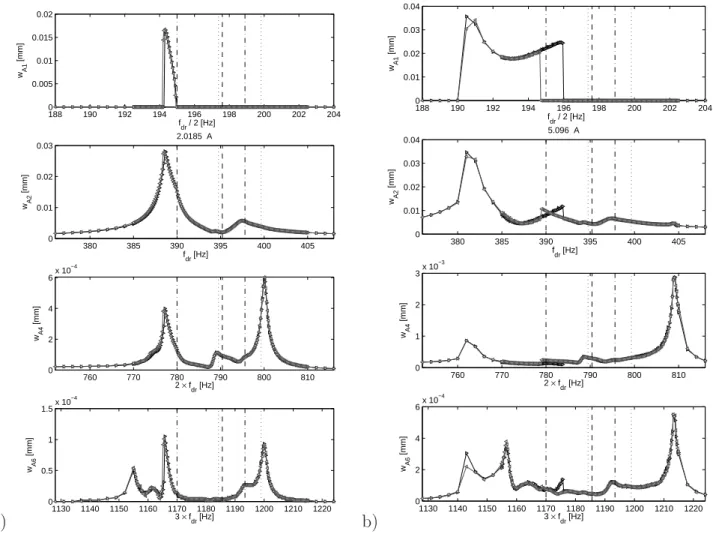
In this section, the driving frequency fdr is selected in the range [380, 405] Hz, where the
degenerates modes with two configurations at 390 Hz and 397.8 Hz, are present (mode and 3). As in the previous section, two forcing amplitudes are shown, I=2 A and I=5A. The signal decomposition by harmonics is also perform to analyze mode couplings, but contrary to the previous case, the lock-in amplifiers are selected at half the driving frequency in order to recover the component oscillating at the fundamental frequency, around fdr/2, in order to measure the
coupling with the fundamental mode. In figure 5, wA1 thus refers to the component at fdr/2
in the vibration, while wA2 denotes the component at the driving frequency. For the analysis,
we also add in the figure the sixth harmonic wA1 (oscillating at three times the excitation
fre-quency).
For the moderate amplitude of forcing (I=2A), one can observe that the 1:2 internal resonance between the first configuration (directly excited) at 390 Hz and the fundamental mode, is ex-cited, giving rise to energy transfer and the occurrence of a component wA1. On the other
hand, the second configuration is not enough excited to activate the coupling with the funda-mental, so that a 1:2 resonance scenario is here present. On the other hand, around the second configuration, a clear coupling with the modes at 4f1 is observed as denoted by the important
19th
International Congress on Sound and Vibration, Vilnius, Lithuania, July 8–12, 2012
two upper modes at 789.5 and 799.3 Hz, is observed, but it seems that the frequency range between these two energy transfers (1:2 and 1:2:2) is enough separated to assume two different coupled dynamics. Finally, wA6 shows an important peak at 1155 Hz which is not slave to other
component, so that one can assume that cubic nonlinearities are already active for this range of amplitude and a small amount of energy is transferred via 1:3 resonance between wA2 and
wA6.
For the larger amplitude (I=5A), the two identified couplings are still present, with now a strong hysteresis in the response between forward and backward sweep in the first 1:2 reso-nance, leading to jum phenomena. Morevoer, the frequency range of that 1:2 resonance now overlaps the frequency band where the coupling with wA6 is observed, so that a 1:2:6 scenario
should be assumed. As in figure 4(b), the positions of the solution branches are slighlty shifter to the low-frequencies, indicating a global softening behaviour and the excitation of cubic non-linearity. a) 188 190 192 194 196 198 200 202 204 0 0.005 0.01 0.015 0.02 wA1 [mm] fdr / 2 [Hz] 380 385 390 395 400 405 0 0.01 0.02 0.03 wA2 [mm] fdr [Hz] 2.0185 A 760 770 780 790 800 810 0 2 4 6x 10 −4 wA4 [mm] 2 × f dr [Hz] 1130 1140 1150 1160 1170 1180 1190 1200 1210 1220 0 0.5 1 1.5x 10 −4 wA6 [mm] 3 × fdr [Hz] b) 188 190 192 194 196 198 200 202 204 0 0.01 0.02 0.03 0.04 wA1 [mm] fdr / 2 [Hz] 380 385 390 395 400 405 0 0.01 0.02 0.03 0.04 wA2 [mm] f dr [Hz] 5.096 A 760 770 780 790 800 810 0 1 2 3x 10 −3 wA4 [mm] 2 × f dr [Hz] 1130 1140 1150 1160 1170 1180 1190 1200 1210 1220 0 2 4 6x 10 −4 wA6 [mm] 3 × fdr [Hz]
Figure 5. Frequency response curves for I=2A (left column) and I=5A (right column), excitation frequency fdr in the vicinity of the second mode. First line: component at half
the driving frequency. Second, third and fourth lines: component at the driving frequency fdr, 2fdr
and 3fdr. Forward (− ⊲ −) and backward (− ⊳ −) frequency sweeps. Linear eigenfrequency markers
f1 (– –) ; 2f1 (– · –) and 4f1 (· · · ·)
3.
Model fitting to experiment
In order to gain insight into the complicated dynamics exhibited by the steelpan in forced vibrations, a simple model involving three internally resonnant modes presenting a 1:2:2 rela-tionship, is used to fit the experimental FRFs. When the driving frequency is in the vicinity of the fundamental mode, analytical solutions are accessible via multiple scales analysis [2]. These will be used to fit the unknown nonlinear coupling coefficients and obtain a better identification of the energy transfers in the first case analysed in section 2.2.1 (Fig. 4).
The three-modes model reads:
¨ q1+ ω 2 1q1 = ε [−2µ1˙q1− α1q1q2− α2q1q3+ F1cos Ωt] (1a) ¨ q2+ ω 2 2q2 = ε h −2µ2˙q2− α3q 2 1 i (1b) ¨ q3+ ω 2 3q3 = ε h −2µ3˙q3− α4q 2 1 i (1c)
where Ω = 2πfdr, qk denotes the modal amplitude of mode k, ωk= 2πfk its angular frequency
and µk and µk its damping coefficient. These values are extracted from the linear analyses
performed in section 2.1. Considering the first experiment, we have Ω ≃ ω1, and ω2 ≃ 2ω1,
ω3 ≃ 2ω1. The amplitude of the forcing is deduced from the measurement, and the nonlinear
coupling coefficients αi are fitted from experimental FRFs.
a) 188 190 192 194 196 198 200 202 204 206 0 0.005 0.01 0.015 0.02 0.025 0.03 0.035 0.04 WA1 [mm] f dr [Hz] 375 380 385 390 395 400 405 410 0 0.5 1 1.5 2 2.5 3 3.5 4 x 10⁻³ WA2 [mm] 2 × f dr [Hz] b) 188 190 192 194 196 198 200 202 204 206 0 0.01 0.02 0.03 0.04 0.05 0.06 WA1 [mm] f dr [Hz] 375 380 385 390 395 400 405 410 0 0.005 0.01 0.015 WA2 [mm] 2 × f dr [Hz]
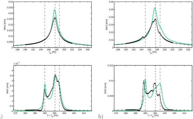
Figure 6. Experimental fitting by a 1:2:2 multiple scale model. Frequency response curves for I=1A (left column) and I=2A (right column), excitation frequency fdr ≃ f1. Harmonics 1 and 2
of the measured displacement wA. Linear eigenfrequency markers f1 (– –) and 2f1 (– · –)
The best fit obtained is shown in figure 6, where two forcing amplitudes are represented, I=1A (a smaller value as compared to the first case shown in figure 6) and I=2A (corresponding to figure 6(a). For the smaller amplitude (I=1A), one can see that the model fairly recovers all the features of the FRF. The discrepancies can be easily attributed to the non-modelled presence of the fourth mode. As noted in section 2.2.1, a 1:2:2:4 coupling is observable. Con-sequently, more energy is transferred from the directly excited mode that has to feed also the
19th
International Congress on Sound and Vibration, Vilnius, Lithuania, July 8–12, 2012
fourth mode in the experiment. This explains the fact that the model overpredict the maxi-mum vibration amplitude of wA1. Secondly, the presence of the mode at 4f1 also explains the
more complicated shape of the FRF for wA1 in the vicinity of 396 Hz. The discrepancies are
enhanced when increasing the forcing amplitude to I=2A. The overprediction of the maximum amplitude in wA1 is larger, as a reflection of the fact that more energy has been transferred to
the non-modelled fourth mode, which response is more significant, contributing in the impor-tant peak around 395 Hz for wA2.
This fitting shows that simple models can be used to enhance the comprehension of the complicated dynamics experimentally observed. The model displaying 1:2:2 internal resonance allows to recover the main feature of the FRFs, while non-modelled effect appears to be easily interpreted. The most complete model for that case should be a 1:2:2:4 one, unfortunately analytical solutions for that problem are not tractable. Further work will consider fitting models of 1:2 and 1:2:2 to the high frequency excitation shown in figure 5. Other notes of the steelpan are also investigated.
4.
Conclusion
Nonlinear vibrations of one note of a steelpan have been experimentally investigated. Forced vibrations have been used to gain a better comprehension of the different mode couplings. The main features found by this experimental analysis are the following :
- Nonlinear coupling and energy exchange are excited for very small vibration amplitudes, of the order of 1/25 the thickness
- Numerous modes displaying internal resonances are present and excited, hence resulting in a complex, high-dimensional dynamics
- Fine analysis allows to isolate features of 1:2:2, 1:2:4 and 1:2:4:6 internal resonances
- Cubic nonlinearity appears not negligible for the usual amplitudes of vibrations encountered - Simple models can be used to explain the most important features of the FRFs
In normal playing, all these features are simultaneously excited, giving rise to a rich tone with a build-up of frequency through energy transfers and a complicated dynamics involving from 3 to 10 modes, resulting in the peculiar and interesting sound of the steelpan.
REFERENCES
1
A. Achong. Mode locking on the non-linear notes of the steelpan. Journal of Sound and Vibration, 266:193–197, 2003.
2
M. Monteil, C. Touz´e, O. Thomas, and J. Frelat. Vibrations non lin´eaires de steelpans : couplages modaux via la r´esonance interne 1:2:2. In 20`eme congr`es fran¸cais de m´ecanique (Besan¸con), 2011.
3
A.H. Nayfeh. Nonlinear Oscillations. Wiley Classics Library, 1979.
4
T. D. Rossing, Hansen Uwe J., and D. S. Hampton. Vibrational mode shapes in Caribbean steelpans. I. Tenor and double second. Journal of the acoustical society of america, 108(2):803–812, 2000.
5
O. Thomas, C. Touz´e, and A. Chaigne. Asymmetric non-linear forced vibrations of free-edge cicular plates. Part 2: experiments. Journal of Sound and Vibration, 265:1075–1101, 2003.