Characterization of carotid artery plaques using noninvasive vascular ultrasound elastography

(1)

Université de Montréal

Characterization of Carotid Artery Plaques Using

Noninvasive Vascular Ultrasound Elastography

par Hongliang Li

Département de pharmacologie et physiologie/Institut de génie biomédical/Faculté de médecine

Thèse présentée en vue de l’obtention du grade de Philosophiae Doctor (Ph.D.) en génie biomédical

September 2019

(2)

Faculté des études supérieures et postdoctorales

Cette thèse intitulée :

Characterization of Carotid Artery Plaques Using Noninvasive Vascular Ultrasound Elastography

Présentée par : Hongliang Li

a été évalué par un jury composé des personnes suivantes :

Fréderic Leblond, Ph.D. Président-rapporteur Guy Cloutier, Ph.D. Directeur de recherche Samuel Kadoury, Ph.D. Membre du jury Siddhartha Sikdar, Ph.D. Examinateur externe Alain Vinet, Ph.D.

(3)

Résumé

L'athérosclérose est une maladie vasculaire complexe qui affecte la paroi des artères (par l'épaississement) et les lumières (par la formation de plaques). La rupture d'une plaque de l'artère carotide peut également provoquer un accident vasculaire cérébral ischémique et des complications. Bien que plusieurs modalités d'imagerie médicale soient actuellement utilisées pour évaluer la stabilité d'une plaque, elles présentent des limitations telles que l'irradiation, les propriétés invasives, une faible disponibilité clinique et un coût élevé. L'échographie est une méthode d'imagerie sûre qui permet une analyse en temps réel pour l'évaluation des tissus biologiques. Il est intéressant et prometteur d’appliquer une échographie vasculaire pour le dépistage et le diagnostic précoces des plaques d’artère carotide. Cependant, les ultrasons vasculaires actuels identifient uniquement la morphologie d'une plaque en termes de luminosité d'écho ou l’impact de cette plaque sur les caractéristiques de l’écoulement sanguin, ce qui peut ne pas être suffisant pour diagnostiquer l’importance de la plaque. La technique d’élastographie vasculaire non-intrusive (« noninvasive vascular elastography (NIVE) ») a montré le potentiel de détermination de la stabilité d'une plaque. NIVE peut déterminer le champ de déformation de la paroi vasculaire en mouvement d’une artère carotide provoqué par la pulsation cardiaque naturelle. En raison des différences de module de Young entre les différents tissus des vaisseaux, différents composants d’une plaque devraient présenter différentes déformations, caractérisant ainsi la stabilité de la plaque.

Actuellement, les performances et l’efficacité numérique sous-optimales limitent l’acceptation clinique de NIVE en tant que méthode rapide et efficace pour le diagnostic précoce des plaques vulnérables. Par conséquent, il est nécessaire de développer NIVE en tant qu’outil d’imagerie non invasif, rapide et économique afin de mieux caractériser la vulnérabilité liée à la plaque. La procédure à suivre pour effectuer l’analyse NIVE consiste en des étapes de formation et de post-traitement d’images. Cette thèse vise à améliorer systématiquement la précision de ces deux aspects de NIVE afin de faciliter la prédiction de la vulnérabilité de la plaque carotidienne.

(4)

l’imagerie par oscillations transversales couplées à deux estimateurs de contrainte fondés sur un modèle de déformation fine, soit l’ « affine phase-based estimator (APBE) » et le « Lagrangian speckle model estimator (LSME) », ont été évaluées. Pour toutes les études de simulation et in

vitro de ce travail, le LSME sans imagerie par oscillation transversale a surperformé par rapport

à l'APBE avec imagerie par oscillations transversales. Néanmoins, des estimations de contrainte principales comparables ou meilleures pourraient être obtenues avec le LSME en utilisant une imagerie par oscillations transversales dans le cas de structures tissulaires complexes et hétérogènes.

Lors de l'acquisition de signaux ultrasonores pour la formation d'images, des mouvements hors du plan perpendiculaire au plan de balayage bidimensionnel (2-D) existent. Le deuxième objectif de cette thèse était d'évaluer l'influence des mouvements hors plan sur les performances du NIVE 2-D (Chapitre 6). À cette fin, nous avons conçu un dispositif expérimental in vitro permettant de simuler des mouvements hors plan de 1 mm, 2 mm et 3 mm. Les résultats in vitro ont montré plus d'artefacts d'estimation de contrainte pour le LSME avec des amplitudes croissantes de mouvements hors du plan principal de l’image. Malgré tout, nous avons néanmoins obtenu des estimations de déformations robustes avec un mouvement hors plan de 2.0 mm (coefficients de corrélation supérieurs à 0.85). Pour un jeu de données cliniques de 18 participants présentant une sténose de l'artère carotide, nous avons proposé d'utiliser deux jeux de données d'analyses sur la même plaque carotidienne, soit des images transversales et longitudinales, afin de déduire les mouvements hors plan (qui se sont avérés de 0.25 mm à 1.04 mm). Les résultats cliniques ont montré que les estimations de déformations restaient reproductibles pour toutes les amplitudes de mouvement, puisque les coefficients de corrélation inter-images étaient supérieurs à 0.70 et que les corrélations croisées normalisées entre les images radiofréquences étaient supérieures à 0.93, ce qui a permis de démontrer une plus grande confiance lors de l'analyse de jeu de données cliniques de plaques carotides à l'aide du LSME.

Enfin, en ce qui concerne le post-traitement des images, les algorithmes NIVE doivent estimer les déformations des parois des vaisseaux à partir d’images reconstituées dans le but d’identifier les tissus mous et durs. Ainsi, le dernier objectif de cette thèse était de développer un algorithme d'estimation de contrainte avec une résolution de la taille d’un pixel ainsi qu'une efficacité de calcul élevée pour l'amélioration de la précision de NIVE (Chapitre 7). Nous avons

(5)

proposé un estimateur de déformation de modèle fragmenté (SMSE) avec lequel le champ de déformation dense est paramétré avec des descriptions de transformées en cosinus discret, générant ainsi des composantes de déformations affines (déformations axiales et latérales et en cisaillement) sans opération mathématique de dérivées. En comparant avec le LSME, le SMSE a réduit les erreurs d'estimation lors des tests de simulations, ainsi que pour les mesures in vitro et in vivo. De plus, la faible mise en œuvre de la méthode SMSE réduit de 4 à 25 fois le temps de traitement par rapport à la méthode LSME pour les simulations, les études in vitro et in vivo, ce qui pourrait permettre une implémentation possible de NIVE en temps réel.

Mots-clés : Athérosclérose, plaque vulnérable, élastographie par ultrasons, oscillations transversales, imagerie par ondes planes, mouvements hors plan, imagerie à haute résolution, transformées en cosinus discret, modèle clairsemé, flux optique, estimation de phase, estimation de contraintes affines.

(6)

Abstract

Atherosclerosis is a complex vascular disease that affects artery walls (by thickening) and lumens (by plaque formation). The rupture of a carotid artery plaque may also induce ischemic stroke and complications. Despite the use of several medical imaging modalities to evaluate the stability of a plaque, they present limitations such as irradiation, invasive property, low clinical availability and high cost. Ultrasound is a safe imaging method with a real time capability for assessment of biological tissues. It is clinically used for early screening and diagnosis of carotid artery plaques. However, current vascular ultrasound technologies only identify the morphology of a plaque in terms of echo brightness or the impact of the vessel narrowing on flow properties, which may not be sufficient for optimum diagnosis. Noninvasive vascular elastography (NIVE) has been shown of interest for determining the stability of a plaque. Specifically, NIVE can determine the strain field of the moving vessel wall of a carotid artery caused by the natural cardiac pulsation. Due to Young’s modulus differences among different vessel tissues, different components of a plaque can be detected as they present different strains thereby potentially helping in characterizing the plaque stability.

Currently, sub-optimum performance and computational efficiency limit the clinical acceptance of NIVE as a fast and efficient method for the early diagnosis of vulnerable plaques. Therefore, there is a need to further develop NIVE as a non-invasive, fast and low computational cost imaging tool to better characterize the plaque vulnerability. The procedure to perform NIVE analysis consists in image formation and image post-processing steps. This thesis aimed to systematically improve the accuracy of these two aspects of NIVE to facilitate predicting carotid plaque vulnerability.

The first effort of this thesis has been targeted on improving the image formation (Chapter 5). Transverse oscillation beamforming was introduced into NIVE. The performance of transverse oscillation imaging coupled with two model-based strain estimators, the affine phase-based estimator (APBE) and the Lagrangian speckle model estimator (LSME), were evaluated. For all simulations and in vitro studies, the LSME without transverse oscillation imaging outperformed the APBE with transverse oscillation imaging. Nonetheless, comparable

(7)

or better principal strain estimates could be obtained with the LSME using transverse oscillation imaging in the case of complex and heterogeneous tissue structures.

During the acquisition of ultrasound signals for image formation, out-of-plane motions which are perpendicular to the two-dimensional (2-D) scan plane are existing. The second objective of this thesis was to evaluate the influence of out-of-plane motions on the performance of 2-D NIVE (Chapter 6). For this purpose, we designed an in vitro experimental setup to simulate out-of-plane motions of 1 mm, 2 mm and 3 mm. The in vitro results showed more strain estimation artifacts for the LSME with increasing magnitudes of out-of-plane motions. Even so, robust strain estimations were nevertheless obtained with 2.0 mm out-of-plane motion (correlation coefficients higher than 0.85). For a clinical dataset of 18 participants with carotid artery stenosis, we proposed to use two datasets of scans on the same carotid plaque, one cross-sectional and the other in a longitudinal view, to deduce the out-of-plane motions (estimated to be ranging from 0.25 mm to 1.04 mm). Clinical results showed that strain estimations remained reproducible for all motion magnitudes since inter-frame correlation coefficients were higher than 0.70, and normalized cross-correlations between radiofrequency images were above 0.93, which indicated that confident motion estimations can be obtained when analyzing clinical dataset of carotid plaques using the LSME.

Finally, regarding the image post-processing component of NIVE algorithms to estimate strains of vessel walls from reconstructed images with the objective of identifying soft and hard tissues, we developed a strain estimation method with a pixel-wise resolution as well as a high computation efficiency for improving NIVE (Chapter 7). We proposed a sparse model strain estimator (SMSE) for which the dense strain field is parameterized with Discrete Cosine Transform descriptions, thereby deriving affine strain components (axial and lateral strains and shears) without mathematical derivative operations. Compared with the LSME, the SMSE reduced estimation errors in simulations, in vitro and in vivo tests. Moreover, the sparse implementation of the SMSE reduced the processing time by a factor of 4 to 25 compared with the LSME based on simulations, in vitro and in vivo results, which is suggesting a possible implementation of NIVE in real time.

(8)

Keywords : Atherosclerosis, vulnerable plaque, ultrasound elastography, transverse oscillations, plane wave imaging, out-of-plane motions, high-resolution imaging, discrete cosine transforms, sparse model, optical flow, phase estimation, affine strain estimation.

(9)

List of tables

Table 2-1 Comparison of imaging modalities ... 19 Table 5-1 List of abbreviations ... 47 Table 6-1 The dimension parameters of a carotid bifurcation phantom with a soft plaque with 70% stenosis... 81 Table 7-1 Computation efficiency (second/frame). ... 123

(16)

List of figures

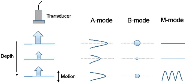
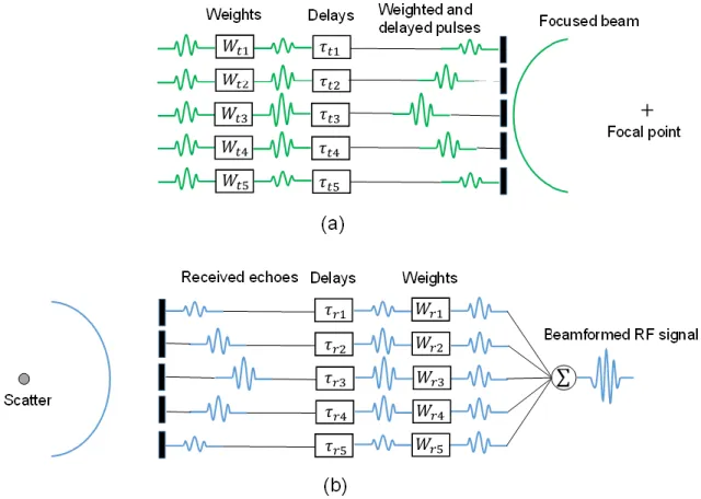
Figure 2.1 Atherosclerosis pathogenesis. Damaged endothelium (A). Fatty streak formation (B). Adapted and modified from [28]. ... 8 Figure 2.2 AHA classification of atherosclerotic lesions. Flow chart in the second column presents the progression of atherosclerotic lesions. Roman numbers indicate lesion types which are described in the first column. The loop between types V and VI clarifies how lesions are enlarged when thrombi deposit on their surfaces repeatedly. Adapted from [29]. ... 9 Figure 2.3 Diagram of cross-sectional morphology of AHA lesion classification. Adapted and modified from [29]. ... 10 Figure 2.4 Micrograph of a carotid plaque from an asymptomatic patient. A large lipid core and a thin fibrous cap are presented. Adapted from [31]. ... 11 Figure 2.5 DSA image of a carotid internal artery with a severe stenosis. Adapted and modified from [48]. ... 12 Figure 2.6 An IVUS image of an internal carotid artery acquired by a 30 MHz transducer. A hyperechoic region (open arrow) suggests a calcification. Hypoechoic plaque is seen at the shoulder of the lesion (short arrows). Adapted and modified from [53]. ... 13 Figure 2.7 Raw (A), logarithm (B) OCT and histology (C) images of a fibroatheroma with less macrophages in the fibrous cap. Raw (D), logarithm (E) OCT and histology (F) images of a fibroatheroma with more macrophages in the fibrous cap. Adapted from [54]. ... 14 Figure 2.8 An echolucent plaque indicated by the yellow arrow causing 70% stenosis. ECA = external carotid artery, ICA = internal carotid artery, CCA = common carotid artery, STA = superficial temporal artery. Adapted from [56]. ... 15 Figure 2.9 Plaque component analysis of a 75-year-old man with a transient ischemic attack using CT image reconstruction software. Volume-rendered image where the carotid artery is traced (A). Reconstruction post-processed image (B). Plaque cross-sectional identification positioned in (B), as indicated by white arrows (C), (D) and (E), where the lumen is indicated by a red contour, the lipid component by the red color, mixed tissues in green and calcium in blue. Adapted from [57]. ... 16 Figure 2.10 Pre-contrast T1-weighted image (A), post-contrast T1-weighted images (B, C). Histological image (D) indicating the fibrous cap by the green contour and LRNC by the yellow

(17)

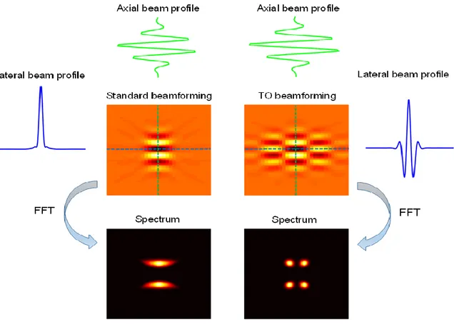
contour. Micrographs regarding regions in (D) that are showing a strong contrast enhancement (E, F). Adapted from [60]. ... 17 Figure 2.11 Shear strain elastogram of a plaque with 60% stenosis of internal carotid artery in a cross-sectional view. Adapted from [70]. ... 18 Figure 3.1 Gray-scale imaging modes. Display examples of A-mode, B-mode and M-mode with respect to static and moving objects. ... 22 Figure 3.2 An image formation process using line-by-line focused imaging. The number of scan lines for one image is typically 256. Adapted from [71]. ... 23 Figure 3.3 A diagram of delay and sum beamforming for transmitting (a) and receiving (b) phases using a linear transducer whose five elements are excited. The limited number of elements considered is just for the purpose of display. ... 24 Figure 3.4 Beam shapes generated by a linear transducer with six active elements using unfocused beam steering (a), focusing without beam steering (b), focusing with beam steering (c), no apodization (d) and apodization (e). ... 26 Figure 3.5 Principle of synthetic aperture imaging. In transmitting, each element sends a spherical wave sequentially spreading throughout the entire scan plane. In receiving, all elements of a transducer acquire echoes. For each transmitting and receiving event, channel data are reconstructed into a low resolution image using DAS approach. Finally, all low resolution images are summed into a high resolution image. ... 28 Figure 3.6 Principle of coherent plane wave imaging. In transmission, several tilting plane waves are generated using all transducer elements activated by linear delays. In receiving, all transducer elements acquire echoes. For each transmission and receiving event, channel data are beamformed into a low resolution image. Finally, all low resolution images at different tilting angles are coherently summed into a high resolution image. ... 30 Figure 3.7 Beamformed images and corresponding frequency spectra using standard and TO beamforming, respectively. Lateral and axial beam profiles indicated by blue and green lines are shown respectively. ... 31 Figure 4.1 Principle of ultrasound strain imaging. A minute compression is applied on a soft phantom with a hard inclusion. Two RF signals, pre-compression and post-compression signals, are acquired and analyzed to obtain displacements at each depth. Finally, the spatial gradient of

(18)

Figure 4.2 Diagram of window-based motion estimation. A measurement window with size of 𝑀 × 𝑁 defined in a reference frame is tracked within a searching region of a target frame. The motion vector of the image block is estimated using some similarity metrics. ... 35 Figure 5.1 (a) The choice of TO filtering parameters using different pairs of 𝜆𝑥 and 𝜎𝑥. Here the test range of 𝜆𝑥 is from 0.4 mm to 1 mm and that for 𝜎𝑥 is from 0.2 mm to 1 mm, with 0.1 mm increment. From this simulation, 𝜆𝑥 = 0.5 mm and 𝜎𝑥 = 0.4 mm provided the smallest estimation deviation (NRMSE) for principal strains and these values were chosen as the TO filtering parameters in our study. (b) The corresponding filtering mask. ... 59 Figure 5.2 B-mode images and principal strains for a simulated vascular phantom with one soft inclusion and four hard inclusions. First row: the CPWC image and CPWC&TO image. Second row: ground truth of the principal minor strains from finite-element model and the principal minor strain estimated with the APBE on CPWC&TO data, the APBE using the time-ensemble approach on CPWC&TO data, the APBE using the incompressibility constraint and the time-ensemble approach on CPWC&TO data, the LSME using the time-time-ensemble approach on CPWC&TO data, the LSME using the incompressibility constraint and the time-ensemble approach on CPWC&TO data, and the LSME using the incompressibility constraint and the time-ensemble approach on CPWC data, whose NRMSE are 14.2%, 13.0%, 10.6%, 9.0%, 8.6%, 8.4%, respectively. Third row: ground truth of the principal major strains from finite-element model and the principal major strain estimated with the APBE and LSME using the same strategies, whose NRMSE are 17.4%, 14.5%, 12.9%, 9.6%, 9.4%, and 9.5%, respectively. .. 60 Figure 5.3 B-mode images and principal strains of a homogeneous phantom in vitro experiment. First row: the cross-section image of the phantom, the CPWC image and CPWC&TO image. Second row: the principal minor strains estimated with the APBE on CPWC&TO data, the APBE using the time-ensemble approach on CPWC&TO data, the APBE using the incompressibility constraint and the time-ensemble approach on CPWC&TO data, the LSME using the time-ensemble approach on CPWC&TO data, the LSME using the incompressibility constraint and the time-ensemble approach on CPWC&TO data, and the LSME using the incompressibility constraint and the time-ensemble approach on CPWC data, whose SNRs are 11.1 dB, 11.3 dB, 12.0 dB, 15.9 dB, 14.2 dB, 16.5 dB respectively. Third row: the principal

(19)

major strains estimated with the APBE and LSME using the same strategies, whose SNRs are 7.2 dB, 7.5 dB, 12.0 dB, 8.9 dB, 14.2 dB, and 16.5 dB, respectively. ... 62 Figure 5.4 SNRs calculated from principal strains estimated with CPWC&TO + APBE, CPWC&TO + APBET_{, CPWC&TO + APBE}T&I_{, CPWC&TO + LSME}T_{, CPWC&TO +} LSMET&I_{, and CPWC + LSME}T&I_{over a range of applied strains from 0.07% to 4.5%. (a)} Principal minor strains. (b) Principal major strains. Five realizations were considered. ... 63 Figure 5.5 B-mode images and principal strains of a heterogeous phantom in vitro experiment. First row: the cross-section image of the phantom, the CPWC image and CPWC&TO image. Second row: the principal minor strains estimated with the APBE on CPWC&TO data, the APBE using the time-ensemble approach on CPWC&TO data, the APBE using the incompressibility constraint and the time-ensemble approach on CPWC&TO data, the LSME using the time-ensemble approach on CPWC&TO data, the LSME using the incompressibility constraint and the time-ensemble approach on CPWC&TO data, and the LSME using the incompressibility constraint and the time-ensemble approach on CPWC data, whose SNRs are 7.6.dB, 9.5 dB, 18.3 dB, 12.5 dB, 19.4 dB, and 21.1 dB, respectively, and CNRs are -5.2 dB, 4.1 dB, 10.2 dB, -2.6 dB, 11.5 dB, and 16 dB, respectively. Third row: the principal major strains estimated with the APBE and LSME using the same strategies, whose SNR are 9.7 dB, 11.5 dB, 18.3 dB, 12.6 dB, 19.4 dB, and 21.1 dB, respectively, and CNRs are -8.5 dB, 0.4 dB, 10.2 dB, 3.2 dB, 11.5 dB, and 16 dB, respectively. ... 65 Figure 5.6 SNRs and CNRs calculated from principal strains estimated with CPWC&TO + APBE, CPWC&TO + APBET_{, CPWC&TO + APBE}T&I_{, CPWC&TO + LSME}T_{, CPWC&TO +} LSMET&I_{, and CPWC + LSME}T&I_{over a range of applied strains from 0.07% to 3.6%. (a), (b)} SNRs for principal strains. (c), (d) CNRs for principal strains. Five realizations were considered. ... 66 Figure 5.7 The point spread functions (PSF) and corresponding Fourier spectra of CPWC and CPWC&TO beamforming: (a) The PSF of the CPWC image, (b) the PSF of the CPWC&TO image, (c) the Fourier spectrum of (a), (d) the Fourier spectrum of (b). ... 68 Figure 5.8 Performance of the phase-based and optical flow-based estimators to estimate the displacement between a pair of 1-D sinusoidal signals under ideal condition (no noise added) for different displacements along x and y axes. ... 71

(20)

Figure 5.9 Ground truth of motion components from finite-element model (first column) and motion components estimated with the APBE on CPWC&TO beamformed data (second column) and CPWC&TO with heterodyne demodulation data (third column). Note that the incompressibility constraint was not used to better appreciate the influence of the heterodyne demodulation on each motion component. The strain components were also not combined to obtain principal strains for this example. ... 75 Figure 6.1 (a) The mold and vessel core of a carotid bifurcation phantom with a soft plaque with 70% stenosis. (b) The polyvinyl alcohol cryogel phantom... 81 Figure 6.2 In vitro experimental setup diagram. Panel (a) demonstrates longitudinal view acquisitions. Panel (b) displays cross-sectional view acquisitions. ... 82 Figure 6.3 Time-varying maximum strain curves (a) and mean strain curves (b) in longitudinal view. The out-of-plane motions are 0 mm, 1 mm, 2 mm, and 3 mm respectively from left to right. (c) Axial strain maps at peak dilation for the first flow cycle (red circle in (b)) of the segmented plaque superimposed on the reconstructed B-mode images. (d) Axial strain maps at peak compression for the first flow cycle (blue circle in (b)) of the segmented plaque superimposed on the reconstructed B-mode images. ... 87 Figure 6.4 Correlation coefficients of time-varying maximum and mean strain curves regarding different out-of-plane motions in longitudinal view. For maximum strain curves, the correlation coefficients are 0.998, 0.985 ± 0.004, 0.920 ± 0.008 and 0.643 ± 0.158 respectively for out-of-plane motions of 0 mm, 1 mm, 2 mm and 3 mm. For mean strain curves, correlation coefficients are 0.999, 0.979 ± 0.016, 0.953 ± 0.021 and 0.818 ± 0.019 respectively for out-of-plane motions of 0 mm, 1 mm, 2 mm and 3 mm. ... 88 Figure 6.5 Time-varying maximum strain curves (a) and mean strain curves (b) in cross-sectional view. The out-of-plane motions are 0 mm, 1 mm, 2 mm, 3 mm respectively from left to right. (c) Axial strain maps at peak dilation for the first flow cycle (red circle in (b)) of the segmented plaque superimposed on the reconstructed B-mode images. (d) Axial strain maps at peak compression for the first flow cycle (blue circle in (b)) of the segmented plaque superimposed on the reconstructed B-mode images. ... 90 Figure 6.6 Correlation coefficients of time-varying maximum and mean strain curves regarding different out-of-plane motions in cross-sectional view. For maximum strain curves, the

(21)

correlation coefficients are 0.997, 0.964 ± 0.002, 0.857 ± 0.023 and 0.608 ± 0.087 respectively for out-of-plane motions of 0 mm, 1 mm, 2 mm and 3 mm. For mean strain curves, the correlation coefficients are 0.999, 0.982 ± 0.002, 0.919 ± 0.005 and 0.832 ± 0.004 respectively for out-of-plane motions of 0 mm, 1 mm, 2 mm and 3 mm. ... 91 Figure 6.7 Examples of axial strain maps at peak compression of the segmented plaques superimposed on reconstructed B-mode images of clinical data with mean out-of-plane motions of 0.37 mm (a), 0.64 mm (c) and 0.90 mm (e). Corresponding time-varying mean strain curves and normalized cross-correlation (NCC) curves of motion-compensated RF images (b), (d) and (f)... 92 Figure 6.8 Correlation coefficients of mean strain curves regarding out-of-plane motion ranges of 0.24 - 0.51 mm, 0.51 - 0.78 mm, and 0.78 – 1.05 mm, whose sample sizes are 5, 7 and 6 participants, respectively. Correlation coefficients are 0.796 ± 0.096, 0.768 ± 0.043 and 0.744 ± 0.044, respectively, and corresponding mean normalized cross-correlation (NCC) values are 0.954 ± 0.013, 0.947 ± 0.026 and 0.936 ± 0.022 for these three groups of out-of-plane motions. ... 93 Figure 6.9 Correlation coefficients of time-varying maximum and mean strain curves regarding different out-of-plane motions in longitudinal view using the Ultrasonix scanner (L14-5/38 probe) for in vitro experiments. For maximum strain curves, correlation coefficients are 0.945, 0.907 ± 0.034, 0.838 ± 0.035 and 0.560 ± 0.015 for out-of-plane motions of 0 mm, 1 mm, 2 mm and 3 mm, respectively. For mean strain curves, correlation coefficients are 0.964, 0.955 ± 0.036, 0.904 ± 0.028 and 0.803 ± 0.062 for the same out-of-plane motions, respectively. ... 94 Figure 6.10 Correlation coefficients of time-varying maximum and mean strain curves regarding different out-of-plane motions in longitudinal view using the Verasonics scanner (L7-4 probe) with focused imaging and coherent plane wave compounding (CPWC) imaging for in vitro experiments considering out-of-plane motions of 0 mm, 1 mm, 2 mm and 3 mm. For maximum strain curves using focused imaging, correlation coefficients are 0.985, 0.877 ± 0.029, 0.800 ± 0.011 and 0.599 ± 0.061, respectively. For mean strain curves using focused imaging, correlation coefficients are 0.992, 0.973 ± 0.010, 0.873 ± 0.007 and 0.691 ±

(22)

0.014, respectively. For maximum and mean strain curves using CPWC imaging, correlation coefficients have been reported in figure 6.4. ... 95 Figure 6.11 Correlation coefficients of maximum and mean axial shear curves regarding different out-of-plane motions in longitudinal view. For maximum shear curves, correlation coefficients are 0.991, 0.970 ± 0.007, 0.877 ± 0.016 and 0.590 ± 0.185 respectively for out-of-plane motions of 0 mm, 1 mm, 2 mm and 3 mm. For mean shear curves, correlation coefficients are 0.999, 0.973 ± 0.010, 0.950 ± 0.012 and 0.720 ± 0.016 respectively for out-of-plane motions of 0 mm, 1 mm, 2 mm and 3 mm. ... 100 Figure 6.12 Correlation coefficients of maximum and mean axial shear curves regarding different out-of-plane motions in cross-sectional view. For maximum shear curves, correlation coefficients are 0.999, 0.981 ± 0.003, 0.973 ± 0.004 and 0.811 ± 0.126 respectively for out-of-plane motions of 0 mm, 1 mm, 2 mm and 3 mm. For mean shear curves, correlation coefficients are 0.998, 0.983 ± 0.004, 0.966 ± 0.005 and 0.807 ± 0.144 respectively for out-of-plane motions of 0 mm, 1 mm, 2 mm and 3 mm. ... 100 Figure 6.13 Correlation coefficients of mean axial shear curves for small, moderate and large out-of-plane motions of clinical images, which are 0.879 ± 0.037, 0.865 ± 0.058 and 0.832 ± 0.106, respectively, for these three groups of out-of-plane motions. Corresponding mean normalized cross-correlation (NCC) values are 0.954 ± 0.013, 0.947 ± 0.026 and 0.936 ± 0.022, respectively... 101 Figure 7.1 (a) B-mode image of an artery simulation model with one soft inclusion and four hard inclusions. The image SNR is 20 dB. (b), (c) Principal minor and major strains of the finite-elements model ground truth. (d), (e) Principal minor and major strains using LSME, whose NRMSE are 8.45% and 9.56%, respectively. (f), (g) Principal minor and major strains using SMSE, whose NRMSE are 6.75% and 7.02%, respectively. Close-ups in the red rectangular regions are displayed to present the resolution of strain maps. ... 117 Figure 7.2 (a), (b) B-mode images with a SNR of 10 dB and corresponding principal strain maps. (c), (d) B-mode images with a SNR of 15 dB and corresponding principal strain maps. NRMSEs of principal strain maps with the LSME and SMSE are shown. ... 118 Figure 7.3 B-mode images with a global SNR of 20 dB and local noise at a SNR of 5 dB in the upper left (a), upper right (b), lower left (c) and lower right (d) regions and corresponding

(23)

principal strain maps. NRMSEs of principal strain maps with the LSME and SMSE are shown. ... 119 Figure 7.4 (a) B-mode image of a homogeneous vascular phantom. (b), (c) Principal minor and major strains using the LSME, whose residual strains are -0.49% and 0.49%, respectively. (d), (e) Principal minor and major strains using the SMSE, whose residual strains are -0.14% and 0.13%, respectively. ... 120 Figure 7.5 (a) B-mode image of a heterogeneous vascular phantom with a soft inclusion under the lumen. (b), (c) Principal minor and major strains using the LSME, whose residual strains are -0.56% and 0.56%, respectively. (d), (e) Principal minor and major strains using the SMSE, whose residual strains are -0.19% and 0.17%, respectively. ... 121 Figure 7.6 (a) In vivo B-mode image of a carotid artery of a 30 year-old healthy male. (b), (c) Principal minor and major strains using the LSME, whose residual strains are -5.56% and 5.56%, respectively. (d), (e) Principal minor and major strains using the SMSE, whose residual strains are -1.92% and 1.77%, respectively. ... 122 Figure 7.7 (a) Mean strain curve of cumulated principal minor strains for the LSME and SMSE over two cardiac cycles. (b) Mean strain curve of the cumulated principal major strain for the LSME and SMSE over two cardiac cycles. ... 122 Figure 7.8 Two successive cardiac cycles of cumulative principal strain curves were selected from figure 7 to perform linear regressions for (a) principal minor strains of the LSME and SMSE, and (b) principal major strains of the LSME and SMSE... 123 Figure 7.9 (a) B-mode image of a soft phantom with three sizes of hard inclusions of 2 mm, 1 mm and 0.8 mm. (b), (c), (d) axial strains using the LSME with a 1.0 mm × 1.0 mm window size and 50%, 80% and 95% overlaps, respectively. (e) axial strains using the SMSE. ... 124 Figure 7.10 (a) B-mode image of a soft phantom with three hard inclusions of 2 mm at different depths. (b) axial strains using the LSME with a 1.0 mm × 1.0 mm window size and 80% overlap. (c) axial strains using the SMSE. ... 124

(24)

List of symbols

𝑐 : The speed of sound 𝑍 : Acoustic impedance

R : Acoustic reflection coefficient 𝐷𝑑𝑒𝑝𝑡ℎ : Maximum imaging depth

𝜏 : The time delays applied on transducer elements

𝑑_{𝑝𝑖𝑡𝑐ℎ} : The distance between two adjacent transducer elements 𝜃 : The steering or tilted angle of plane wave transmission

𝑟 : Pixel intensities of the reference frame

𝑟̅ : The mean intensity of pixels inside the measure window from the reference frame 𝑡 : Pixel intensities of the target frame

𝑡̅ : The mean intensity of pixels inside the measure window from the target frame 𝐼𝑥 : The spatial derivative of image intensity in the lateral direction

𝐼_𝑧 : The spatial derivative of image intensity in the axial direction 𝐼_𝑡 : The derivative of image intensity in the temporal direction 𝑈𝑥 : Lateral displacement

𝑈𝑧 : Axial displacement 𝑠_𝑥𝑥 : Lateral strain 𝑠𝑥𝑧 : Lateral shear strain 𝑠_𝑧𝑥 : Axial shear strain 𝑠_𝑧𝑧 : Axial strain

Θ : The phase of a cross-spectrum

𝑘𝑥 : The frequency variable in the lateral direction 𝑘_𝑧 : The frequency variable in the axial direction

𝑓𝑥 : The modulated spatial frequency in the lateral direction 𝑓_𝑧 : The modulated spatial frequency in the axial direction

(25)

𝜆𝑧 : The transmitted pulse wavelength

𝜎𝑥 : The full width at half maximum of a Gaussian envelope

Φ : The phase difference of two Fourier spectrums 𝜙 : The phase of an analytical image

𝑛𝑡 : The time-ensemble length

Δ𝑡 : The time step between two consecutive frames

E : Elasticity modulus

𝛾 : Poisson’s ratio

𝜀_𝑚𝑖𝑛 : Principal minor strain 𝜀𝑚𝑎𝑥 : Principal major strain 𝑑𝑖𝑣 : Divergence operator

𝜆𝑑 : The regularization parameter to regulate the influence of incompressibility constraint 𝜆_𝑠 : The regularization parameter to regulate the influence of smoothness constraint 𝐜_𝐱 : The coefficients of Discrete Cosine Transform of a lateral displacement field 𝐜_𝐲 : The coefficients of Discrete Cosine Transform of an axial displacement field B : The Discrete Cosine Transform matrix

𝐁𝒙_{: The first-order derivative of B in the lateral direction} 𝐁𝒚_{: The first-order derivative of B in the axial direction} 𝐷̇ : First-order derivative operator

(26)

List of abbreviations

CT : Computed tomography

MRI : Magnetic resonance imaging IVUS : Intravascular ultrasound CEUS : Contrast-enhanced ultrasound OCT : Optical coherence tomography DSA : Digital subtraction angiography PET : Positron emission tomography

SPECT : Single photon emission computed tomography NIRF : Near-infrared fluorescence

NIVE : Noninvasive vascular elastography RF : Radiofrequency

CPWC : Coherent plane wave compounding TO : Transverse oscillation

CPWC&TO : Coherent plane wave compounding with transverse oscillation beamforming CPWC&TO* : CPWC with TO beamforming and heterodyne demodulation

LSME : Lagrangian speckle model estimator LSMET_{: LSME with the time-ensemble approach}

LSMET&I_{: LSME with the time-ensemble approach and the incompressibility constraint} PBE : Phase-based estimator

APBE : Affine phase-based estimator

APBET_{: APBE with the time-ensemble approach}

APBET&I_{: APBE with the time-ensemble approach and the incompressibility constraint} SMSE : Sparse model strain estimator

FWHM : Full width at half maximum HS : Horn-Schunck

LK : Lucas-Kanade OF : Optical flow ROI : Region of interest

(27)

AHA : American Heart Association LRNC : Lipid-rich necrotic core IPH : Intraplaque hemorrhage LRNC : Lipid-rich necrotic core PSV : Peak systolic velocity CCA : Common carotid artery ICA : Internal carotid artery ECA : External carotid artery HU : Hounsfield unit

DAS : Delay and sum

ARFI : Acoustic radiation force impulse NCC : Normalized cross-correlation LSQSE : Least squares strain estimator MW : Measurement window

PVA-C : Polyvinyl alcohol cryogel

NRMSE : Normalized root-mean-square-error RoCLT : Range of cumulated lateral translation MaxSCs : Maximum strain curves

MeanSCs : Mean strain curves DCT : Discrete Cosine Transform

(28)

(29)

Acknowledgements

First of all, I would like to thank my research supervisor, Professor Guy Cloutier, who offered me a chance to work in Laboratoire de biorhéologie et d'ultrasonographie médicale (LBUM). His creative opinions and broad knowledge inspired me throughout my research. Without his wise advices and support, I would not finish this thesis. I believe that the scientific rigor and perseverance gained from him will encourage me throughout my career.

I am grateful to Professor Fréderic Leblond, Professor Samuel Kadoury, Professor Siddhartha Sikdar and Professor Alain Vient for kindly accepting as my defense committee members.

Special thanks to Dr. Louise Allard for her support on my study and life.

I also would like to thank Université de Montréal, l’Institut de Génie Biomédical de l’Université de Montréal and Réseau de Bio-Imagerie du Québec for their scholarship support.

Thanks to other coauthors of my papers, Dr. Jonathan Porée, Dr. Marie-Hélène Roy-Cardinal, Boris Chayer, Judith Muijsers, Marcel van den Hoven, Zhao Qin, Professor Gilles Soulez and Professor Richard Lopata for their collaborations and contributions.

I say thank you to previous and present LBUM members. I learned a lot from your expertise. It was my pleasure to work with you.

I especially want to thank some friends who I met in Montréal. Shiming, Meng, Qian, Boxuan, Lei, Shanshan, Wei, Linjiang, Qi, Yu, Huiyang, Shuiling, Huicheng and all others. I really enjoyed the time we spent.

Finally, I would like to thank my family for their unwavering support and endless love. Also, I wish my father could receive my appreciation in paradise for his love. Additionally, I present this work to my upcoming son.

(30)

Chapter 1 : General introduction

1.1 Motivation

Atherosclerosis is a progressive disease affecting large blood vessels such as coronary, peripheral or carotid arteries. It is characterized by the accumulation of lipids and fibrous deposits inside intimal regions of the vessel wall [1]. As the lipid accumulates in the intima, a plaque is gradually formed to induce vessel inward remodeling followed by a decrease of the vessel lumen. As a consequence, the narrowed vessel lumen affects the quantity of blood distributed downstream, and the insufficient supply of blood could lead to ischemic stroke when carotid arteries are considered. On the other hand, the biomechanical instability of a plaque may also induce ischemic complications. Indeed, an unstable (vulnerable) plaque, which is prone to rupture, is characterized by a lipid core and a thin fibrosis cap infiltrated by macrophages [2]. Following rupture, a thrombus may form in the blood stream and when it is detaching of the wall by the flow kinetics, it can migrate and obstacle downstream smaller arteries, causing ischemic stroke.

In current clinical practice, the level of luminal vessel narrowing or stenosis degree is commonly used as an indicator of treatments to prevent stroke. Specifically, patients with mild or moderate stenosis (less than 70% in diameter reduction) are recommended to change lifestyle or take medication. Severe stenoses are treated by carotid endarterectomy or angioplasty. However, the severity of carotid artery stenosis is not sufficient to identify plaques at high risk of rupture. One-third of cryptogenic stroke whose origin is unknown is induced by rupture of non-stenotic but high risk plaques [3]. On the other hand, some patients with a severe stenosis may never experience any symptoms and are thought to have stable plaques [4]. In other words, defining the vulnerability of a plaque is a multifactorial process [5], involving not only the plaque geometry, but also its composition [6]. Thus, comprehensive and early diagnosis of plaque vulnerability has its clinical value for stroke prevention.

Several approaches are currently used to evaluate the atherosclerosis progression. Angiography can detect a stenosis, but it fails to provide information about the content of the plaque. Computed tomography (CT) methods are able to assess the degree of stenosis and the

(31)

amount of calcium in the plaque, but accurate identification and quantification of plaque components are challenging because of the limited temporal, spatial, and contrast resolutions. It is also ionizing for patients. Finally, Magnetic resonance imaging (MRI), which is considered the gold standard method to identify lipid-rich tissue, is able to identify vulnerable carotid plaques. But the scan is time-consuming and expensive. Therefore, there is a need to develop a noninvasive, fast and low cost imaging tool to better characterize the plague vulnerability.

Safety, real time and easy accessibility of ultrasound enable it as a method of choice for screening and diagnosis of vascular plaques. Clinically, Doppler imaging is used to evaluate a stenosis using the peak systolic velocity [7]. Indeed, an obstructed vessel results in the acceleration of the blood flow. However, this method cannot provide information on the composition of a plaque. To gain this information, several techniques based on ultrasound echo properties were utilized. Intravascular ultrasound (IVUS) can image the vessel wall and provide volume information of plaques using a catheter with an ultrasound transducer on the extremity, but this technique is invasive. Contrast-enhanced ultrasound (CEUS) is a way to image intraplaque neovessels using microbubbles, which are associated with the growth of plaques. One drawback of CEUS is the injection of contrast agents within the venous system. Another limitation is that it is still insufficient to detect the lipid core and fibrosis cap of a vulnerable plaque.

Ultrasound elastography or strain imaging, a method first introduced by Ophir et al. [8] in 1991, is a technique that measures the strain or relative elasticity of biological tissues,. An external compression is applied on a tissue and its displacements responding to the stress are measured with a tracking method. Strains can be obtained from the spatial derivation of displacements. In the late nineties, elastography was explored to characterize the vessel wall with IVUS images. The natural cardiac pulsation or the inflation of a compliant balloon on a catheter was used by de Korte et al. [9] to differentiate the coronary calcified plaque component (less strain) from non-calcified tissues (higher strain) in vivo. However, IVUS elastography is invasive, which restricts it to be a complementary tool of B-mode IVUS for assessing vascular plaques. In 2004, noninvasive vascular elastography (NIVE) was proposed to show the potential of determining the stability or vulnerability of a plague using ultrasound imaging [10]. NIVE

(32)

caused by the natural cardiac pulsation without the need of an external compression. Due to Young’s modulus differences among different vessel tissues, a lipid pool, a calcified and a normal tissue made of collagen and elastin are expected to present different strains under the blood pressure stress activation.

Currently, sub-optimum performance and computational efficiency limit the clinical acceptance of NIVE as a fast and efficient method for the early diagnosis of vulnerable plaques. Specifically, NIVE with a cross-sectional view of the vessel is challenging because the motion perpendicular to the ultrasound beam, namely the lateral motion, is difficult to track because of the limited lateral resolution of ultrasound images and the absence of phase information in that direction. To improve the estimation performance of NIVE, developments of new strain algorithms and advanced ultrasound image reconstruction methods were made.

To improve lateral strain estimation, Konofagou et al. [11] proposed to perform interpolation between adjacent radiofrequency (RF) A-lines. A one-dimensional (1-D) cross-correlation based method was used to obtain high precision lateral displacements [12]. The main disadvantage of this 1-D method is that the accuracy of the lateral displacement estimation is lower by an order of magnitude, compared with the axial displacement estimation, because of differences between lateral and axial resolutions. To avoid noisy lateral estimation, the spatial angular compounding strategy was proposed to reconstruct radial and circumferential strains using only accurate axial estimations at several steering angles [13-15]. However, these approaches compute strains from displacement derivatives, which enhances variance of strain estimations due to associated high frequency displacement noise. To circumvent this issue, an alternative strategy is the affine model-based estimation, which derives all strain components, such as axial, lateral and shear strains, directly without derivative operations [16-18]. Nevertheless, lateral strain estimation is still not reliable using these affine models [19].

Advanced ultrasound beamforming methods could also improve lateral strain estimation. Korukonda and Doyley demonstrated that synthetic aperture imaging enhanced lateral displacement estimation with a cross-correlation based method [20, 21]. Coherent plane wave compounding (CPWC) beamforming was also proposed to obtain superior lateral strain estimation with the model-based Lagrangian speckle model estimator (LSME) [18]. Recently, a transverse oscillation (TO) beamforming strategy provided improved lateral displacement

(33)

estimations for vascular and cardiac applications [17, 22]. In the context of cross-sectional NIVE, however, the performance of model-based strain estimators considering advanced beamforming, such as CPWC and TO imaging, has not yet been studied.

Another important challenge for strain estimation is the inherent issue of out-of-plane motion. During 2-D ultrasound acquisitions, out-of-plane motions that are perpendicular to the imaging scan plane are not considered, consequently they may impact the reliability of NIVE because vascular wall motions are three-dimensional (3-D). The magnitude of out-of-plane motions is hypothesized to induce strain estimation artifacts due to reduced image correlation. Based on simulations, Fekkes et al. [23] demonstrated that a 3-D cross-correlation based strain estimator outperformed 2-D methods when large out-of-plane motions were considered. A similar conclusion was made by Brusseau et al [24]. In that latter study, a multi-row probe was devised to achieve multi-plane acquisitions. A maximum out-of-plane motion of 0.8 mm was considered using a breast mimicking phantom and a 3-D search scheme. However, to our knowledge, there has been no study on the influence of out-of-plane motions for NIVE using in

vitro and in vivo clinical dataset. Moreover, an evaluation framework to determine the impact

of out-of-plane motions on the performance of estimation methods is a necessity for clinical 2-D NIVE.

The computation efficiency is another issue that needs to be addressed. Most strain estimation algorithms are window-based. Specifically, pre-and post-motion images are divided into overlapping windows. Then, cross-correlation [14, 21] or affine [18, 25] estimations are performed within each window. To solve the whole motion field, motion parameters of each window are estimated successively. However, there is always a trade-off between the window size, window overlapping and computation efficiency. Larger windows and overlaps result in more accurate motion estimation with higher spatial resolution, but at a cost of a higher computation time. Low computation efficiency may limit NIVE for clinical screening and characterization of vulnerable plaques. To reduce computation, a global estimation strategy could be an option. Some global approaches, such as the Horn-Schunck (HS) optical flow algorithm [26], consider all pixels inside a region of interest (ROI) to solve a dense motion field globally. Those schemes usually require to optimize iteratively a cost function until convergence

(34)

optimization process into a least squares scheme to obtain analytic solutions of the Doppler vector domain [27]. The impact of this idea on improving computation efficiency deserves to be investigated for NIVE.

1.2 Objectives

The procedure to perform NIVE analysis consists in image formation and image post-processing steps. Specifically, image formation, also called beamforming, is a process to transmit and receive ultrasound echoes and to reconstruct images using reflected signals from moving vessels. Thereafter, using a technology of motion tracking, the image post-processing allows to compute the motion or strain field of vessel walls from reconstructed images. This thesis aims to improve the accuracy of these two aspects of NIVE to facilitate predicting carotid plaque vulnerability.

First of all, regarding image formation, conventional line-by-line focused imaging is the technique implemented on most scanners for clinical examination. Emerging imaging modalities, such as plane wave imaging, are promising to enhance image quality. Some other specific imaging technologies, such as transverse oscillation beamforming, were proven efficient for motion tracking due to enriching lateral phase information. This approach may thereby improve the performance of ultrasound elastography. Therefore, the first objective of this thesis was to introduce these novel imaging approaches into NIVE. The advantages of advanced imaging methods coupled with model-based strain estimators are expected to improve NIVE performance.

Secondly, during the acquisition of ultrasound RF signals for image formation, the carotid artery is deformed in 3-D. When performing 2-D NIVE, we assume that the carotid artery is only moving in a 2-D scan plane. Thus, 2-D NIVE suffers from the influence of plane motions. The next objective of this thesis was to investigate the influence of out-of-plane motions on the performance of 2-D NIVE. This knowledge could give new guidelines for the clinical use of NIVE.

Finally, regarding image post-processing, NIVE algorithms need to estimate strains of vessel walls from reconstructed images with the objective of identifying soft and hard tissues.

(35)

Although a large amount of strain estimation algorithms have been proposed, a strain estimator that is able to determine subtle structures inside a carotid artery is still needed. Therefore, the third objective of this thesis was to develop a strain estimation algorithm with a high resolution as well as a high computation efficiency.

1.3 Thesis plan

This thesis consists of eight chapters. Beside the present introduction (Chapter 1) that gives the motivation and objectives of this work, Chapter 2 presents the pathophysiology of carotid atherosclerosis, including its causes and symptoms. It also introduces diagnosis tools to characterize carotid plaques. Chapter 3 presents the basic principles of ultrasound image formation and undertakes a literature review of emerging ultrasound imaging modalities, whereas Chapter 4 provides a state of the art introduction to ultrasound elastography and, especially, details of approaches used for NIVE. Chapter 5 consists in the first article of this thesis, which applied plane wave and transverse oscillation beamforming into the image formation to evaluate NIVE performance with two strain estimation algorithms. Chapter 6 is the second article of this thesis, which established a framework for evaluating out-of-plane motions and discussed the influence of such artifact motions on NIVE performance. Chapter 7 includes the third article of this thesis, which aims to fulfill our third objective. A strain estimation algorithm based on a sparse model is proposed to reconstruct a dense strain field with pixel-wise resolution as well as a high computation efficiency. Finally, Chapter 8 discusses originalities and limitations of my doctoral works, concludes the whole three projects and gives future perspectives.

(36)

Chapter 2 : Atherosclerosis

2.1 Atherosclerosis pathogenesis

Atherosclerosis is a vascular disease that affects artery walls (by thickening) and lumens (by plaque formation). Before introducing the method of diagnosis and the characterization of the vulnerability of the plaque, it is worthwhile to better understand its pathogenesis.

A healthy artery wall consists of three layers: tunica intima, tunica media and tunica adventitia, as shown in figure 2.1(A). The tunica intima, commonly called the intima, is the innermost layer, mainly made up of a single layer of endothelial cells. It is a permeable barrier that performs the exchange between the blood and the artery wall. The tunica media is the middle layer and normally the thickest part of the artery wall. Smooth muscle cells, its primary component, regulate dilation and compression of the artery. The outermost layer, the tunica adventitia, consists of collagenous and elastic fibers. This layer helps the artery to attach with surrounding tissues.

The exact mechanism of the pathogenesis of atherosclerosis is still not clearly understood. However, a widely acceptable theory on the cause of atherosclerosis is a response to an injury, as shown in figure 2.1(A). This theory claims that atherosclerosis is initiated by subtle physical devastation of endothelial cells due to some risk factors (e.g., hypertension, diabetes, infections, etc...). This injury process provokes an inflammatory response as monocytes adhere to the damaged endothelial layer and then entered beneath, which induces thickening of the intima. As proliferation of low-density lipoproteins (LDL) goes on at the site of the injury, monocytes would differentiate into macrophages and start to ingest LDL, which would induce intimal thickening. The macrophages containing LDL, also referred to as foam cells, are the main part of the fatty streak, as shown in figure 2.1(B). These fatty streaks are asymptomatic and consist in the precursor stage of atherosclerosis. Over time, foam cells die and lipids gradually accumulate into the endothelial layer. This could cause the formation of a fibrous plaque with a lipid-rich necrotic core and an overlying collagen cap.

(37)

Figure 2.1 Atherosclerosis pathogenesis. Damaged endothelium (A). Fatty streak formation (B). Adapted and modified from [28].

2.2 Atherosclerosis progression

The atherosclerotic disease is progressive; it can start in the childhood and progress silently through the elderly. Its pathologic features include three stages corresponding to early, intermediate and advanced lesions defined by the American Heart Association (AHA) [29]. A summary of atherosclerosis progression phases is shown in figure 2.2, in which 6 types of lesions are classified. Initial lesions (type I) and fatty streak lesions (type II) are early lesions, where intimal thickening and intracellular lipid accumulation happen. Type III lesions correspond to an intermediate stage, as shown in figure 2.3(c), where some small pools of extracellular lipid appear in this stage. Type IV lesions (atheroma) represent the first phase of advanced lesions. It arises from the formation of lipid cores as more lipids accumulate (figure 2.3(d)). Type V lesions, referred to as fibroatheroma (figure 2.3(e)), are different from type IV lesions, as a fibrous cap covering a lipid core is formed. The fibrous cap is made of smooth muscle cells and infiltrated by varying amounts of macrophages and lymphocytes [30]. Type VI lesions could be described as the disruption state of type IV and V lesions surface [30]. They not only have the morphology of type IV or V lesions, but they also present surface fissures and/or hemorrhage/hematoma of lesions and/or thrombi (figure 2.3(f)).

(38)

Figure 2.2 AHA classification of atherosclerotic lesions. Flow chart in the second column presents the progression of atherosclerotic lesions. Roman numbers indicate lesion types which are described in the first column. The loop between types V and VI clarifies how lesions are enlarged when thrombi deposit on their surfaces repeatedly. Adapted from [29].

2.3 High-risk plaque description

Thrombosis accompanying plaque rupture is one of the major cause of ischemic stroke in patients with carotid artery atherosclerosis [31]. It is shown that the risk of stroke is annually less than 1% when asymptomatic patients have a stenosis less than 75%, while the risk is increased to 2% - 5% for those with one higher than 75% [32, 33]. For symptomatic patients with severe stenosis (≥ 70%) who suffered from transient ischaemic attacks previously, the risk rises up to 10% for the first year and goes much higher to 30%-35% in the next five years [33, 34].

(39)

Figure 2.3 Diagram of cross-sectional morphology of AHA lesion classification. Adapted and modified from [29].

However, the risk of lesion rupture is not only associated with the size of the lesion, but also with its morphology [35, 36]. A typical morphology of a lesion with a high risk of rupture, also named a vulnerable plaque, is presented in figure 2.4. A vulnerable plaque is characterized by a thin fibrous cap and a large lipid-rich necrotic core (LRNC). The overlying thin fibrous cap is infiltrated by macrophages with few or absence of smooth muscle cells [37]. The thicknesses of the thin fibrous cap of vulnerable carotid plaques vary from 80 𝜇𝑚 – 460 𝜇𝑚 depending on different measurement modalities, including optical coherence tomography (OCT) [38], sonography [39] and post-mortem histopathology [40]. Fissures and ruptures on the thin cap would lead to total disruption of the fibrous cap [35], exposing then the lumen to thrombogenic substances underlying the lipid core [35].

Another main ingredient of a vulnerable plaque is the LRNC that is considered as soft tissues. A large LRNC was identified as a strong predictor of vulnerable plaque fissures [41]. A

(40)

accounts for more than 40% of the plaque area can be considered as a high-risk lesion [42]. Moreover, in a small clinical trial of 37 patients with carotid stenosis larger than 70%, patients with a LRNC were more often symptomatic than asymptomatic [43].

Intraplaque hemorrhage (IPH) is commonly seen in advanced lesions and it is associated with carotid plaque progression [44, 45]. It arises from the disruption of microvessels which could be introplaque neovasculars that stem from tunica adventitia. There is evidence to prove that repeated IPH is contributing to the LRNC expansion [46]. In [47], it was reported that the incidence of IPH in symptomatic patients was 84%, which is much higher than the occurrence of 56% in asymptomatic patients.

Figure 2.4 Micrograph of a carotid plaque from an asymptomatic patient. A large lipid core and a thin fibrous cap are presented. Adapted from [31].

2.4 Imaging modalities

There is a strong clinical interest in imaging plaques and assessing its vulnerability, particularly for asymptomatic patients. Identifying the content of the plaque would help to predict its rupture, determine the treatment and prevent stroke. For symptomatic patients who are taking medications, imaging follow-up of plaques is necessary to evaluate treatments and monitor the evolution of lesions. This section gives a brief review of imaging modalities of carotid plaques. Firstly, some invasive technologies, such as angiography, intravascular ultrasound and optical coherence tomography, are introduced. Then, B-mode ultrasound, Doppler ultrasound, CT and

(41)

MRI, which are noninvasive imaging modalities, are reviewed briefly. Finally, other recent and novel imaging methods are discussed.

2.4.1 Angiography

Digital subtraction angiography (DSA) is a reference standard to assess stenosis severity of an artery. During the intervention, a contrast medium is injected through a catheter that allows to see the vessel architecture. The pre-contrast and post-contrast X-ray images are subtracted to highlight opacified lumens. Then, DSA enables to observe and measure accurately the lumen stenosis. However, it does not allow to see plaque components. Moreover, it is invasive and has ionizing radiation, which could induce some complications, such as stroke when the catheter detaches a portion of the plaque unintentionally. In addition, it not suitable to patients who are allergic to iodic-based contrast agents. An example of DSA of a carotid artery is shown in figure 2.5.

Figure 2.5 DSA image of a carotid internal artery with a severe stenosis. Adapted and modified from [48].

2.4.2 Intravascular ultrasound (IVUS)

IVUS is an invasive imaging technology using a catheter with an ultrasound transducer to give a cross-sectional visualization of a plaque. Like ultrasound B-mode imaging, IVUS is able to provide anatomical information, such as lumen stenosis, eccentric patterns, echolucent

(42)

Conventional IVUS with 20 to 40 MHz transducers provides axial resolution of 70 – 200 𝜇𝑚, lateral resolution of 200 – 400 𝜇𝑚 and an imaging depth of 5 – 10 mm [50-52]. One limitation of IVUS is that its resolution is insufficient to distinguish the thin fibrous cap whose thickness is usually less than 65 𝜇𝑚. Better axial resolution with 40 𝜇𝑚 can be achieved with a 60 MHz transducer (Kodama, ACIST Medical Systems), while imaging depth was reduced accordingly. Recently, higher frequency IVUS transducers operating at 90 – 150 MHz have been developed to counter this problem [52]. The axial resolution can reach 50 𝜇𝑚 and below. However, clinical studies are still needed to validate these new technologies. Figure 2.6 shows an IVUS image of a carotid artery with a plaque.

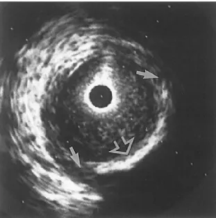
Figure 2.6 An IVUS image of an internal carotid artery acquired by a 30 MHz transducer. A hyperechoic region (open arrow) suggests a calcification. Hypoechoic plaque is seen at the shoulder of the lesion (short arrows). Adapted and modified from [53].

2.4.3 Optical coherence tomography (OCT)

OCT is a high resolution imaging method whose axial resolution is 4 – 20 𝜇𝑚. Its principle is like ultrasound imaging and allows to measure echo time delay and intensity of light scatterers. However, light velocity is much higher than sound speed. One uses low-coherence interferometry to measure the echo time delay indirectly because of such a high speed. The intensity of the backscattered light is recorded to produce a two-dimensional (2-D) image of optical scattering. Due to the superior spatial resolution, OCT is advantageous to measure the