Exchange rate predictability: Taylor rule fundamentals and commodity prices

(1)

Exchange rate predictability: Taylor rule fundamentals and

commodity prices

Gloria, Cleide Mara

GLOC21607503

April 29, 2010

ECN6153: Atélier de macroéconomie

Prof. Marine Carrasco

Département de Sciences Économiques

Université de Montréal

(2)

1 Project Description

The purpose of this research project is to come up with an econometric model that forecasts short-term nominal exchange rates for Canada, Australia, New Zealand, South Africa, and South Korea, vis-à-vis the United States. The currencies of the first four countries are considered “commodity” currencies because natural ressources account for a considerable portion of their exports’ revenue. In contrast, it is South Korea’s imports that are significantly composed of natural ressources. The reason for including South Korea in the study is to see whether or not variations in the price of the commodities have an impact on the exchange rate from both the export and import sides. According to Amano and van Norden (1998), among other factors, variations in the price of the commodities are suspected of influencing the exchange rate through their impact on the terms of trade.

The major inspiration for this study is Molodtsova and Papell (2009)’s paper, which incorporates the Taylor rule in an econometric model to forecast 1-month ahead nominal exchange rates for twelve OECD countries. The model works well for most of the countries but less so for Canada and Australia. The authors attribute this relative worse performance to the nature of these countries’ currencies. This obser-vation provides for the main motiobser-vation of this paper: improve the Taylor rule model given by Molodtsova and Papell for Canada and Australia by incorporating commodity prices in the econometric model, and including the currencies of New Zealand, South Africa, and South Korea, to verify if the currencies of major exporters or importers of natural ressources can be forecasted by the same econometric equa-tion. According to Chen & Rogoff (2003) such a model would be valuable to a developing country whose main source of income is exports of commodities as they move towards a floating exchange rate regime. There is an extensive literature analysing the impact of commodity prices on exchange rate fore-casting. Amano and van Norden (1998) provide evidence that oil prices have a considerable impact on real exchange rates for Canada, although the relationship holds only over long-run horizons. Chen and Rogoff (2003) finds that the US dollar price of the commodity export has a strong influence on floating real rates for Canada, New Zealand, and Australia. Chen (2004) incorporates commodity prices into the classical exchange rate forecasting models for Australia, Canada and New Zealand. She finds that commodity prices improve not only the out-of-sample forecasting performance but also the in-sample fit of the classical models.

As demonstrated by the graphs in appendix A, it appears that real commodity prices are strongly related with nominal exchange rates, especially for Canada, Australia and South Africa, from the early

(4)

80s onward. The relationship is not so evident for New Zealand. This papel further investigates this relationship by focusing on one month-ahead out-of-sample forecasts of the exchange rate of these countries. The exchange rate forecasting model used is the Taylor rule model given by Molodtsova and Papell (2009) completed by each country’s respective commodity price: oil prices for Canada and South Korea, coal prices for Australia, lamb prices for New Zealand and gold prices for South Africa. It turns out that the best evidence that models with commodity prices outperform both the random walk and models without commodity prices is given by Canada and South Africa, followed by Australia and New Zealand. In the case of South Korea, neither the taylor-rule based model from Molodtsova and Papell (2009) nor the commodity prices augmented models outperform the random walk.

2 Theory

2.1 The Taylor rule

The Taylor rule stipulates that central banks pursuing a policy of economic stabilisation, should react to changes in inflation or in output gap by adjusting the short term nominal interest rate in the following manner: if either inflation is above its target and/or output rises above potential output, central banks should raise its nominal interest rate in order to bring the economy back to equilibrium. Clarida et al. (1999, p. 1696) refers to this policy reaction as a “countercyclical response to demand shocks”.

Following Clarida et al. (1999, p. 1695) the Taylor rule is specified as:

i∗_t = α + γπ(πt− ¯π) + γxxt, with α = ¯r + ¯π, γπ > 1, γx> 0 (1)

where i∗

t is the target interest rate, ¯π is the target inflation rate, and ¯r is the long-run equilibrium real

interest rate.

The variable xtrepresents output gap, which is defined as the output that the economy can produce

without raising or lowering the inflation rate. The constants γπ and γx are the weights representing

central banks’ reactions to the variations in the inflation rate and the output gap, respectively. If γπ > γx,

this implies that changes in i∗

t will be higher if a shock is caused by inflation rate deviations from its target

level than by variations in output gap.

In order to derive the econometric forecasting equation , Molodtsova and Papell (2009) states the Taylor rule for the United States as follows:

i∗_t = πt+ φ(πt− π∗) + γyt+ r∗ (2)

where i∗

(5)

of inflation, ytis the output gap, and r∗ is the equilibrium level of the real interest rate.

The Taylor rule for the domestic countries is the same as the one above except that it also includes a term for the real exchange rate qt:

i∗_t = πt+ φ(πt− π∗) + γyt+ r∗+ qt (3)

Following the argument by Clarida et al. (1999) that the Federal Reserve has a tendency to smooth interest rate adjustments, Molodtsova and Papell (2009) allow for the actual observable interest rate it

to partially adjust to the target rate as follows:

it= (1− ρ)i∗t+ ρit−1+ vt (4)

By substituting Eq. (3) into Eq. (4), we get the following equation:

it= (1− ρ)[πt+ φ(πt− π∗) + γyt+ r∗+ δqt] + ρit−1+ vt, with δ = 0 for the US (5)

The interest rate reaction function of the domestic country (Eq. 5) is then subtracted from that of the United States ( Eq. (5) with δ = 0 ). After collecting some terms, we get:

it− ˜it= α + αππt− ˜απ˜πt+ αyyt− ˜αyy˜t+ ρit−1− ˜ρ˜it−1− ˜αqq˜t+ ηt (6)

where ~ denotes variables and coefficients for the domestic countries, and

απ = (1− ρ)(1 + φ), αy = γ(1− ρ), αq= δ(1− ρ), α = (1 − ρ)(φπ∗+ r∗) = constant

Shocks in any of the right-hand side variables in the interest rate differential equation (Eq. 6) will have an impact on the exchange rate. Molodtsova and Papell (2009) makes four predictions:

1. If inflation in the United States rises above the target, the Fed will raise the interest rate to cool down the economy. Higher interest rates lead to an immediate appreciation of the dollar because there will be an influx of foreign capital into the country and thus, an increase the demand for US dollars. According to the overshooting model developed by Dornbusch (1976), which depends on the validity of the Uncovered Interest Rate Parity (UIRP) assumption, the immediate appreciation of the dollar will be followed by a depreciation. Molodtsova and Papell (2009) argue, however, that recent empirical work demonstrates that UIRP does not hold in the short run. Instead, based on the results of Gourinchas and Tornell (2004), Molodtsova and Papell (2009) propose that a rise in interest rates cause an immediate appreciation that continues on. Furthermore, if the other country also follows a Taylor rule, an increase in its inflation will cause the dollar to depreciate since the other country will raise its interest rate and thus attract more foreign capital than the US.

2. If the American output gap increases, the Fed will raise the interest rate causing the dollar to appreciate. If instead, it’s the other country’s output gap that increases, its central bank will raise

(6)

its interest rate, leading to a depreciation of the dollar.

3. If the real exchange rate for the other country depreciates, its central bank will increase the interest rate causing an appreciation of its currency and a depreciatin of the dollar.

4. Assuming there is interest rate smoothing, a higher lagged interest rate increases current and expected future interest rates, which leads to an immediate and sustained dollar appreciation. If, instead, it is the other country’s lagged interest rate that is higher, the dollar would depreciate. The impact on the exchange rate caused by a macroeconomic shock is thus due to changes in the nominal interest rate. In order to directly capture the effects of a shock on the exchange rate, Molodtsova and Papell (2009) combine the four predictions made above with Eq. (6) to produce the Taylor

rule-based exchange rate forecasting equation:

"st+1= ω− ωππt+ ˜ωππ˜t− ωyyt+ ˜ωyy˜t− ωit−1+ ˜ω˜it−1+ ˜ωqq˜t+ ηt (7)

where stis the natural log of the nominal exchange rate, defined as the US dollar price of one unit of the

domestic currency, so that an increase in stis a depreciation of the American dollar.

The reversal of the signs between Eqs. (6) and (7) captures the effect that anything that causes the interest rate in the US to be higher than that of domestic country will lead to an immediate and sustained appreciation of the US dollar (i.e. st decreases). It is not possible to relate the magnitude of

the coefficients of the two equations because it is not known ex-ante how exactly changes in the interest rate differential will impact the exchange rate.

Based on different assumptions about the coefficients, there are sixteen models nested in Eq. (7). These assumptions are:

• Asymmetric (˜ωq #= 0) or symmetric (˜ωq = 0): a symmetric equation means that the domestic

country does not target the exchange rate

• Smoothing (˜ωi #= 0, ωi #= 0) or no smoothing (˜ωi = ωi = 0): no smoothing means that the interest

rate adjusts to its target level within the period.

• Homogeneous coefficients (˜ωπ = ωπ, ˜ωy = ωy, ˜ωi = ωi) or heterogeneous coefficients (˜ωπ #= ωπ,

˜

ωy #= ωy, ˜ωi #= ωi): homogeneous coefficients imply that the impact on the exchange rate caused

by a macroeconomic shock will be the same regardless of the country where the shock originates.

(7)

Now that we know how the Taylor rule can be used to forecast exchange rates, I’ll explain how variations in the international prices of commodities can also have an impact on the exchange rates of Australia, Canada, New Zealand, South Africa and South Korea.

2.2 Commodity prices

For small, open economies such as the ones considered in this paper, the prices for most of their commodity exports are determined in international markets and the volume of their exports do not have an impact on the prices set by these markets; that is, they are price takers. Since commodities represent a large portion of these countries’ exports, fluctuations in commodity prices may lead to fluctuations on the exchange rate through its impact on the country’s terms of trade .

According to Lafrance and Van Norden (1995), a rise in commodity prices leads to improvements in a country’s terms of trade by raising the value of the exports. An increase in exports revenue leads to higher domestic income, which then increases aggregate demand. Higher demand places upward pressure on prices and thus on the inflation rate. If the central bank pursue a policy of economic stability, it will most likely raise interest rates to decrease aggregate demand in order to bring the economy back to equilibrium. As explained in the previous section, an increase in interest rates leads to an appreciation of the country’s currency. Therefore, an increase in the world price of commodities lead to an appreciation (i.e. st increases) of the domestic currency through its impact on the bank’s reaction to increased

aggregate demand.

Chen (2004) gives an additional channel through which commodity prices may affect exchange rates. An increase in the world commodity prices places upward pressures on the domestic prices as explained above. Since prices cannot vary instantaneously, the nominal exchange rate has to depreciate in order to preserve the country’s Purchasing Power Parity (PPP). This can easily be seen by the formula for the real exchange rate. According to the definition of nominal exchange rate used byMolodtsova and Papell (2009) and I, the real exchange rate is defined as1_:

qt= st+ pt− p∗t (8)

where stis the natural log of the nominal exchange rate, p∗t is the natural log of the foreign price level,

and pt is the natural log of the domestic price level. When PPP holds, qt = 0. If there is an upward

pressure on the domestic price level pt , st has to decrease in the short run so as to keep qtconstant.

1_{The note de repère 5 of Prof. Martens clearly specifies how the real exchange is determined according to the different}

(8)

A decrease in st is an appreciation of the American dollar and thus a depreciation of the commodity

currency.

There are thus two opposing forces on the exchange rate as a result of increases on commodity prices. It is not possible to know theoretically which one of these forces dominate the other. The coefficient on commodity price is left positve because that is what Chen (2004) do. Furthermore, there is considerable controverse on whether or not PPP holds so it is more likely that the first effect explained dominates the second.

3 Literature review

3.1 Molodtsova and Papell (2009)

As mentionned in section 2, Molodtsova and Papell (2009) use the Taylor rule-based econometric equa-tion (7) to forecast short-term (1 month) nominal exchange rates for 12 OECD countries vis-à-vis the United States for the post-Bretton Woods period. They compare the out-of-sample predictability of the Taylor rule’s model against a random walk without drift as well as against other conventional exchange rate models such as interest rate differentials, purchasing power parity, and monetary fundamentals. For the one-month-ahead forecasts made by the Taylor rule-based models, Molodtsova and Papell (2009) find statistically significant evidence of exchange rate predictability for 11 out of the 12 OECD countries at the 5% level.

The data used for estimating the forecasting model comes from the IMF’s International Financial Statistics database and run from March 1973 to December 1998 for the Euro zone countries and to June 2006 for the other countries. All data have monthly frequencies except for the seasonally adjusted industrial production for Australia and Switzerland, and the CPI for Australia, which are available only quarterly. The authors then use the “quadratic-match average” option in Eviews 4.0 to convert these series into monthly frequencies.

The output gap is calculated using seasonally adjusted industrial production as a proxy for GDP. The authors use three different trends to compute the output gap: linear trend, quadratic trend and the trend obtained by a Hodrick-Prescott filter. Furthermore, the output gap is calculated in a quasi-real fashion whereby only data up to period t is used to get the output gap at time t. This is done to simulate the reality whereby policy makers use only data that is available to them (i.e. ex-ante) when they make their decisions.

(9)

The authors use data over the period of March 1973 to February 1982 for estimation and save the rest for out-of-sample forecasting. OLS estimation are performed with rolling regressions where the first 120 data points are used and the forecast for the next period is generated. The first data point is then dropped, a data point at the end of the sample is added, and the model is re-estimated. The forecast for the next period is again generated. The process continues on until the last data point in the sample is reached.

As is the standard in the literature since the seminal work by Meese and Rogoff (1983), the out-of-sample performance of the exchange rate forecasting models is evaluated by testing its predictive ability against that of a random walk. The measure of predictive ability most commonly used is the Mean Squared Prediction Error (MSPE). Diebold and Mariano (1995) and West (1996) offer a procedure for testing for predicitive ability based on MSPE comparisons. Molodtsova and Papell (2009) point out, however, that these methods are not applicable in their study because two nested models are being compared. More specifically, the random walk under the null is nested within the model under the alternative (i.e. the model under the alternative becomes the random walk if the coefficients in the alternative model are set equal to zero). According to Molodtsova and Papell (2009), the Diebold and Mariano or the West tests lead to non-normal test statistics when applied to nested models. Instead of these tests, the authors favour the procedure proposed by Clark and West (2006, 2007) to test for predictive ability because the procedure was specifically developed for testing nested models.

As mentionned in section 2, depending on the assumptions made about the coefficients of the fore-casting model, there are sixteen model specifications, each with three different measures of output gap. Therefore, 48 Taylor rule-based models are being estimated for each country to generate inference based on p-values. Such a high volume of estimations could lead to p-values that are overstated. To deal with this issue, Molodtsova and Papell (2009) implement the Hansen’s (2005) test of superior pre-dictability to correct for data snooping. The authors explain that the Hansen test is designed to compare the out-of-sample performance of a benchmark model to that of a set of alternatives. It tests the null that the benchmark model has a higher predictive ability than any of the linear models against the alternative that at least one of the linear models has superior predictive capacity. In Molodtsova and Papell’s case, the benchmark model is the random walk and the set of alternatives are the Taylor-rule based models plus the conventional interest rate, purchasing power parity, and monetary models.

Molodtsova and Papell find statistically significant evidence of short-term exchange rate predictability at the 5% level for 11 out of the 12 OECD countries using models with the Taylor rule. Although the

(10)

predictability results for Canada and Australia are similar to that of the other OECD countries, their US inflation coefficient do not follow the same pattern as the other countries do (near zero from 1983 to 1990 and negative from 1991 to 2006). This means that for Australia and Canada, an increased in US inflation does not lead to an appreciation of the dollar, as the model would predict. The authors argue that this is because Canada and Australia have commodity currencies whose behavior is dominated by factors not common to other industrialized nations. At longer horizons (greater than 3 months), an endnote in the article indicates that there is no evidence of predictability for either the Taylor rule or any of the other conventional models for any of the countries.

The authors find that symmetric models perform better than asymmetric ones. The same is true for models with smoothing as compared to no smoothing. In general, the model specification that produced most short-term predictability is a symmetric model with heterogeneous coefficients, smoothing and a constant.

3.2 Chen and Rogoff (2003)

Finding out whether commodity prices can help predict exchange rates is the focus of Chen and Rogoff (2003)’s article. The authors study the real exchange rate behavior of Canada, Australia, and New Zealand, three small open economies that are “price takers” in world markets for the majority of their commodity exports (that is, the volume of their exports do no have an impact on the world prices of the commodity in question) and whose currencies are labelled “commodity currencies”. According to the authors, in the past decade, commodity products have accounted for 60% of Australia’s exports and more than a half of New Zealand’s. In the case of Canada, more than a quarter of its exports relies on commodity products.

The authors find robust evidence that commodity prices have a significant impact on real exchange rates. Each country real exchange rate is calculated based on three different reference currencies: the US dollar, the British Pound, and a non-US-dollar currency basket.

The commodities chosen reflect major non-energy products produced in each country because the authors argue that Australia, Canada, and New Zealand are not large net exporters of energy commodi-ties. The commodity prices used are quarterly averaged world market prices in US dollars, deflated by the American CPI. Commodity prices indices for each country are then constructed by geometri-cally averaging the deflated commodity prices using the corresponding domestic production share as a weight.

(11)

Chen and Rogoff (2003) use commodity prices instead of standard measures of terms-of-trade (i.e exports divided by imports) because they argue that commodity prices are exogenous whereas standard measures of terms of trade are endogenous. Endogeneity can lead to spurrious relations that do not allow causal interpretation. Indeed, the authors find that except for Canada, terms of trade are strongly correlated with real exchange rates. They also find that standard measures of terms of trade do not react much to movements in world commodity prices. They thus conclude that world commodity prices are much better at capturing exogenous terms-of-trade shocks than standard measures of terms of trade.

3.3 Chen (2004)

In this paper, Chen (2004) uses the fndings from Chen and Rogoff (2003) that commodity prices fluc-tuations can explain real exchange rate behavior and incorporates commodity prices into the classical exchange rate models to improve their in-sample fit and out-of-sample forecasting performance. The countries analyzed are still Australia, Canada and New Zealand. The author uses three different anchor currencies to compute the quarterly nominal exchange rate: the US dollar, the British pound, and the Japanese Yen. She performs out-of-sample forecasts for three horizons: 1, 4, and 8 quarters.

The models used in her paper are:

• Augmented relative Purchase Power Parity (PPP) model:

st= α + βcppcomt + βp(p∗t − pt) + εt

• Augmented asset approach flexible price monetary model:

st= α + βcppcomt + βm(m∗t − mt)− βy(y∗t − yt) + εt • Augmented flexible price monetary model:

st= α + βcppcomt + βm(m∗t − mt)− βy(y∗t − yt) + βi(i∗t − it) + εt • Augmented sticky price monetary model:

st= α + βcppcomt + βm(m∗t − mt)− βy(yt∗− yt) + βi(i∗t − it) + βπ(πt∗− πt) + εt

where pcom

t represents the world price in US dollar of the exported non-energy commodity.

In terms of in-sample estimation, the author find that including commodity prices turns coefficients that are insignificant into significant and positive ones. Including commodity prices thus improves the in-sample fit of the standard models and, furthermore, offers evidence of a long term cointegration relationship between exchange rates and fundamentals.

(12)

With regards to exchange rate predictability, the author finds that the particular specification that have superior forecast ability depend on the anchor currency, the sample period, and the forecast horizon used. She uses rolling regressions to generate out-of-sample forecasts and test the models’ performance against that of random walk (without drift) based on Root Mean Squared Errors (RMSE) comparisons. Including commodity prices can improve the performance of some of the classical models and the performance improves as the forecast horizon increases. However, no single model provide superior predictive performance at all forecast horizons and across all countries.

3.4 Amano and van Norden (1993)

The objective of Amano and van Norden (1993) is to discover whether or not fluctuations in the terms of trade could explain variations in the real exchange rate between Canada and the United States. The authors find that, indeed, there is a cointegration relationship between the real exchange rate and the terms of trade. The authors further establish that causality runs from the terms of trade to the exchange rate, and not vice-versa. Based on these findings, they develop an econometric forecasting equation that outperforms the random walk at short horizons. The equation shows that terms-of-trade fluctuations, as opposed to monetary factors, can explain much of the variation in the real exchange rate since 1973.

The real exchange rate is defined as $CA/$US (i.e. the price in US dollars of one unit of Canadian dollar), deflated using CPIs from both countries. The argument for using the bilateral rate instead of the effective rate is the predominant weight of the US in any effective index for Canada and as well, to be consistent with the monetary models in the literature on exchange rate forecasting.

The terms of trade are defined as commodity exports prices divided by manufactured imports price. The authors split the terms of trade into two components, energy commodities and non-energy com-modities, due to early investigations that showed that energy commodities seems to play a qualitative role different from that of non-energy commodities. Note that the study focuses on out-of-sample fore-casting; the issue of endogeneity is thus not relevant since the authors are not trying to see whether or not the model fits well in-sample (as was the case with Chen and Rogoff (2003)).

The authors point out that it is essential not to use an aggregate measure of the terms of trade but to use commodity and energy terms of trade as distinct variables in the forecasting equation. The relationship between the energy component of the terms-of-trade measure and the real exchange rate could be explained by the fact that the measure of the energy component used also includes energy prices. Amano and van Norden (1993) thus specifies a different measure of terms of trade by using the

(13)

CPI excluding food and energy and find the same results.

Technically speaking, once the authors find that the real exchange rate and the two components of the terms of trade are non-stationary using three different stationarity tests2_{, they establish that the}

real exchange rate and the two terms-of-trade variables are cointegrated. They then construct an error correction model as follows:

"RP F Xt= α(RP F Xt−1− β0− βCT OT COM ODt−1− βET OT EN RGYt−1) + γRDIF Ft−1 (A)

where RPFX is the real exchange rate as defined in the second paragraph, TOTCOMOD and TOTEN-RGY are the non-energy commodity component and the energy component, respectively, of the terms of trade, and RDIFF is the Canada-US interest rate differential used to capture monetary policy’s influence on exchange rates and defined as

RDIF F = (ishort

can − ilongcan)− (ishortus − ilongus ). (B)

Note that the authors also performed stationary tests on RDIFF and found it to be stationary, thus providing some evidence that monetaty policy should have only a transitory effect on the real exchange rate while terms-of-trade shocks should be permanent.

Eq. (A) is estimated up to January 1986 and forecasts for one, three, six and twelve month horizons are generated. The authors then use recursive regressions until the last date (February 1992) is included in the estimation sample. Forecasts are generated each time a new month is included in the sample and Eq. (A) re-estimation is performed. Once all forecasts are computed, forecast errors are calculated for all estimation periods and all horizons. Theil’s U is used to compare the Root Mean Squared Error (RMSE) of the model to that of a random walk.

Amano and van Norden (1993) use different starting dates for their forecasts and find that, in general, Eq. (A) outperforms the random walk at all horizons under consideration and that the model’s perfor-mance improves as the forecast horizon increases. Furthermore, upon employing a variety of tests, the authors conclude that the forecast results are robust and statistically significant and that they are not due to Granger-causality running from the real exchange rate to the independent variables in Eq. (A). That is, it is not shocks in real exchange rates that leads to variations in the terms of trade, but rather the contrary.

Finally, Amano and van Norden (1993), by decomposing the real exchange rate movements, reach three conclusions:

1. RDIFF accounts for only a small portion of real exchange rate variations as opposed to terms-of-2_{The tests are: Augmented Dickey-Fuller, Philips and Perron, and Kwiatkowski, Phillips, Schmidt and Shin.}

(14)

trade shocks.

2. Energy price shocks (i.e. increases or decreases in energy commodity prices) are responsible for most of the exchange rate variation in three out of four sub-periods considered.

3. Large and persistent energy price shocks still have significant effects on the exchange rate fours years later; large but short-lived shocks have negligible impact.

4 Empirical Results

4.1 Data Description

The exchange rate forecasting equation used in this study is the same one proposed by Molodtsova and Papell (2009) but augmented by the country’s specific commodity price: oil prices for Canada and South Korea, coal prices for Australia, lamb prices for New Zealand, and gold prices for South Africa. The country-specific commodity is chosen based on the composition of the commodity price index as found in Chen and Rogoff (2003, p. 158). Crude oil represented 62.3% of the Canadian energy price index from 1972Q1 to 2001Q2 whereas coal represented 73.2% for Australian from 1983Q1 to 2001Q2. For New Zealand, the commodity chosen is lamb because lamb prices accounted for 12.5% of the non-energy commodity index from 1986Q1 to 2001Q2, the highest among all non-energy commodities. I could not find any ready to use commodity price index for South Africa and South Korea. In consequence, the commodity chosen for South Africa is gold because, according to the South African Department of Trade and Industry3_{, it accounted for 18.5% in mining exports in 2009. For South Korea, oil is used because}

this country is a major energy importer.

The general exchange rate forecasting equation used is thus:

"st+1= ω− ωππt+ ˜ωππ˜t− ωyyt+ ˜ωyy˜t− ωiit−1+ ˜ωi˜it−1+ ˜ωqq˜t+ ˜ωpp˜commt+ ηt (9)

where ~ indicates variables and coefficients for countries other than the United States. The variables’ definitions are:

• st: natural log of the nominal exchange rate, defined as the US dollar price of one unit of domestic

currency (i.e. e = $CA/$US), so that an increase in stis a depreciation of the US dollar. • "st+1= st+1− st

(15)

• πt: inflation rate = ln(CP It)− ln(CP It−12)

• yt: output gap (percentage deviation from the trend, using a HP filter). • it−1: interest rate from the previous period.

• qt: natural log of the real exchange rate defined by qt= st+ pt− p∗t, where p∗t stands for the natural

log of the American CPI.

• pcommt: natural log of the country-specific real commodity price deflated by the American CPI

The data for all nominal exchange rates comes from the Federal Reserve Economic Data, collected by the Economic Research Division of Federal Reserve Bank of St. Louis. Note that the nominal exchange rate available at the database did not always follow the definition I use so that I divide 1 by the exchange rates available for Canada, South Africa, and South Korea.

All the data for the remaining variables comes from the International Financial Statistics (IFS) database of the IMF website, with the exception of the New Zealand seasonally adjusted GDP, which comes from Statistic New Zealand.

As in Molodtsova and Papell (2009), I use the “quadratic-match average” option in Eviews 4.0 when-ever I need to convert series that are available quarterly into monthly frequencies. This is the case for the CPI for Australia and New Zealand, the seasonally-adjusted GDP for New Zealand and South Africa, and the seasonally-adjusted industry production for Australia.

Before estimating the forecasting equation (9) given above, it is important to see whether or not the variables are stationary. Non-stationary variables can lead to spurious regression since the asymptotic proprieties of the estimators are no longer valid. The stationary results are discussed next.

4.2 Stationarity Results - variables

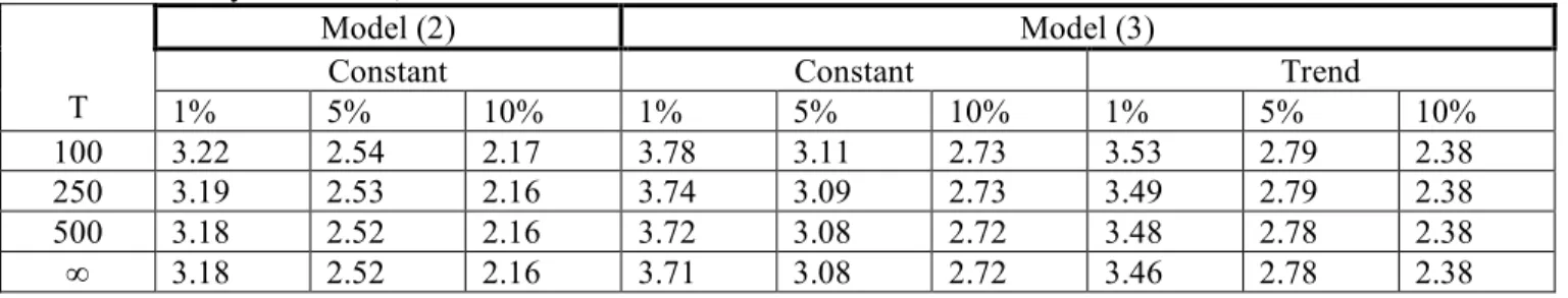
The test used to check for stationarity is the Augmented Dickey-Fuller (ADF) test. To implement the test, the number of lags to use needs to be determined beforehand. The Bayes Information Criterion (BIC) is used to identify which lag would be the best to use to test for stationarity. For each series, an ADF regression is performed using multiple lags. The chosen lag is the one whose BIC has the lowest value. Once the lag is chosen, there are three possible models that could represent the data generating process. MODEL 1 is a series without a constant and without a trend, MODEL 2 is a series without a

(16)

In order to decide among these models, ADF regressions are run on the series with the lowest BIC assuming MODEL 3 holds, and the critical values from the ADF table 2 (model 3 column) found in

Appendix B are used to test whether or not the trend of the series with the lowest BIC is statistically significant. If the trend is significant this implies that the series can be represented by MODEL 3 since

the constant will automatically be significant as well. If the trend is not significant, a new ADF regression without trend is performed to test for the statistically significance of the constant. If the constant is significant (table 2, model 2 column), the series can be represented byMODEL2; otherwise,MODEL1 is

chosen.

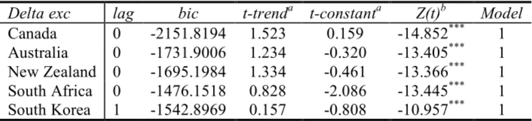
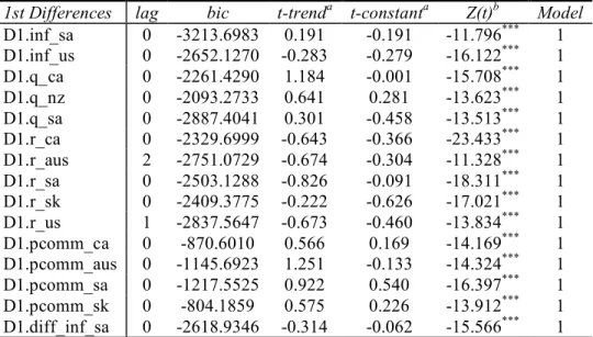
Once the lag and the model are chosen, an ADF test is again performed to test for the unit root. Based on the Dickey-Fuller critical values found in table 1 in appendix B, if the unit root is rejected, the variable is stationary (or, integrated of order 0), otherwise, it is non-stationary. If the variable is found to be non-stationary, the entire ADF procedure is repeated on the first difference of the non-stationary series. If the null of unit root is rejected, the variable is then deemed to be integrated of order 1 or I(1).

The results for all variables can be found in appendix C. All variables are represented by the ADF

MODEL 1 except for the Australia’s inflation and real exchange rates, and South Korea’s real exchange

rate, which, depending on the significance level used, can also be represented by MODEL 2.

Nonethe-less, regardless of the ADF model chosen for these countries, the variables are stationary at either the 10 or 5% significance level. Once again, the Dickey-Fuller critical values used are those from table 1 in appendix B.

A summary of the relevant results is presented in the table below:

Table A: Stationarity results for variables found in Eq. (9)

Canada Australia New Zealand South Africa South Korea US

∆st+1 I(0), 1% I(0), 1% I(0), 1% I(0), 1% I(0), 1% N.A.

πt I(0), 10% I(0), 10% I(0), 10% I(1), 1% I(0), 5% I(1), 1%

yt I(0), 1% I(0), 1% I(0), 1% I(0), 1% I(0), 1% I(0), 1%

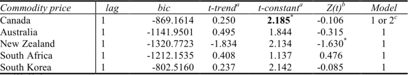
qt I(1), 1% I(0), 10% I(1), 1% I(1), 1% I(0), 10% N.A

i_t−1 I(1), 1% I(1), 1% I(0), 5% I(1), 1% I(1), 1% I(1), 1% pcommt I(1), 1% I(1), 1% I(0), 10% I(1), 1% I(1), 1% N.A.

˜

π_{− π}t I(0), 1% I(0), 1% I(0), 1% I(1), 1% I(0), 1% N.A.

˜

yt− yt I(0), 1% I(0), 1% I(0), 1% I(0), 1% I(0), 1% N.A.

(17)

As shown by the table above, the stationary results are country-specific, except for the dependent variable ∆st+1and the output gap yt, which are stationary for all countries. All contries but South Africa

and the US have the inflation rate πt stationary. The real exchange rate qt, the interest rate it−1, and

the commodity price pcommt are non-stationary for most contries. For all countries, all variables that are

found to be non-stationary taken at their level, are found to be stationary in their first difference, thus integrated of order 1.

The last three rows of the table gives the stationary results for the cases where Eq. (9) have homo-geneous coefficients. Homohomo-geneous coefficients imply that the United States and the domestic country have the same exchange rate elasticities: a shock on inflation rate, output gap, or interest rate will have the same impact on the exchange rate regardless of the country where the shock originated. These variables will be used when estimating the forecasting models in the next section. Note that this is not a hypothesis likely to hold, but nonetheless, homogeneous coefficients are estimated because they are part of the assumptions made in section 2.1.

4.3 Estimation and Forecasts

The general econometric forecasting model used for each country is given by Eq. (9) and reproduced below for convenience:

"st+1= ω− ωππt+ ˜ωππ˜t− ωyyt+ ˜ωyy˜t− ωiit−1+ ˜ωi˜it−1+ ˜ωqq˜t+ ˜ωpp˜commt+ ηt

As noted by Molodtsova and Papell (2009), depending on the assumptions made about the coef-ficients, there are sixteen models embedded within the above equation. As previously stated, these assumption are:

• asymmetric (˜ωq #= 0) or symmetric (˜ωq = 0)

• smoothing (˜ωi #= 0, ωi #= 0) or no smoothing (˜ωi = ωi = 0)

• homogeneous coefficients (˜ωπ = ωπ, ˜ωy = ωy, ˜ωi = ωi) or heterogeneous coefficients (˜ωπ #= ωπ,

˜

ωy #= ωy, ˜ωi#= ωi)

• no constant (ω = 0) or with a constant (ω #= 0)

(18)

Model 1: asymmetric, with no smoothing, homogeneous coefficients , with a constant Model 2: asymmetric , with no smoothing , homogeneous coefficients , without a constant Model 3: asymmetric with no smoothing, heterogeneous coefficients, with a constant Model 4: asymmetric with no smoothing, heterogeneous coefficients, without a constant Model 5: asymmetric with smoothing, homogeneous coefficients, with a constant

Model 6: asymmetric with smoothing, homogeneous coefficients, without a constant Model 7: asymmetric with smoothing, heterogeneous coefficients, with a constant Model 8: asymmetric with smoothing, heterogeneous coefficients, without a constant Model 9: symmetric with no smoothing, homogeneous coefficients, with a constant Model 10: symmetric with no smoothing, homogeneous coefficients, without a constant Model 11: symmetric with no smoothing, heterogeneous coefficients, with a constant Model 12: symmetric with no smoothing, heterogeneous coefficients, without a constant Model 13: symmetric with smoothing, homogeneous coefficients, with a constant

Model 14: symmetric with smoothing, homogeneous coefficients, without a constant Model 15: symmetric with smoothing, heterogeneous coefficients, with a constant Model 16: symmetric with smoothing, heterogeneous coefficients, without a constant 4.3.1 Methodology

The methodology used for estimation and forecast is the same as in Molodtsova and Papell (2009). For each country, one-month-ahead forecasts for each of the 16 models are constructed based on OLS rolling regressions beginning on 1980m14_{. Each model is initially estimated using the first 120 data}

points and the one-month-ahead forecast is generated. The first data point is then dropped, an additional data is added at the end of the sample and the model is re-estimated. A one-month-ahead forecast is generated at each step. The last 120 data points estimated is for the period 1999m9 – 2009m8, which

(19)

generates the forecast for the last date (2009m9). The forecasting period is accordingly 1990m1 to 2009m95_.

To evaluate the out-of-sample performance of the models, Mean Squared Prediction Error (MSPE) is calculated once the forecasting exercise is finished. As is the standard in the literature since Meese and Rogoff (1983), the MSPEm of each model is compared to the MSPErw of a martingale difference

process (random walk without drift). If the MSPE of the random walk is smaller than the model’s MSPE, than the model forecasts worse than a random walk. Statistical tests are performed to test the null H0:

MSPEm = MSPErw against the alternative H1: MSPErw > MSPEm. Rejecting the null means that the

model performs better than a random walk.

According to Molodtsova and Papell (2009), the procedure proposed by Diebold and Mariano (1995) or by West (1996) to construct t-type statistics based on the sample MSPE cannot be used in our case because the model under the null (the random walk) is nested within the model under the alternative. That is, if some (or all) coefficients of the alternative model are set equal to zero, then the alternative model becomes the randon walk model. In this context, the resulting statistic would not have a standard normal distribution. Instead, the authors and I use the MSPE-adjusted procedure proposed by Clark and West (2006, 2007) to construct CW statistics that can be used to compare nested models. The CW statistics is described in the following section.

4.3.2 Clark and West (CW) statistics

In order to test the null of equal predictability against the alternative of linear predictability, a statistic test is performed as proposed by Clark and West (2006, 2007). The general specification of the test is given by Clark and West (2007) while Clark and West (2006) is specific for testing against the random walk. Below is a brief technical summary about the test as given by Clark and West (2007).

Let:

• MODEL 1 be the parsimonious model (i.e. models without commodity prices) • MODEL 2 be the larger, nested model

• yˆ1t+1 be the period t forecast of t+1 of MODEL1

• yˆ2t+1 be the period t forecast of t+1 of MODEL2

5_{Due to data unavailability the forecasting period for New Zealand is 1999m3 to 2009m9 and for South Korea is 1991m4 to}

(20)

• yt+1: be the actual value at t+1 (in this paper, yt+1 ="st+1) • P be the number of predictions made6

• T+1: be the number of observations in the sample

Then, the following variables are defined:

• MSPE1= P−1!T_{t=T−P +1}(yt+1− ˆy1t+1)2

• MSPE2= P−1!T_{t=T−P +1}(yt+1− ˆy2t+1)2

Clark and West (2006, 2007) demonstrate that under the null, MSPE1 is smaller than MSPE2 by

con-struction because MODEL 1 is a more parsimonious model. To overcome this disadvantage, they

pro-pose adjusting MSPE2by an adjustment amount they calculate to be: • Adj = P−1!T_{t=T−P +1}(ˆy1t+1− ˆy2t+1)2

The test then becomes:

• H0: MSPE1= (MSPE2 - Adj)

• H1: MSPE1> (MSPE2 - Adj)

For one month ahead forecasts, Clark and West (2007) suggest the following procedure to implement the test. Let:

• fˆt+1= (yt+1− ˆy1t+1)2−[(yt+1− ˆy2t+1)2−(ˆy1t+1− ˆy2t+1)2], which after some simple algebra becomes:

• fˆt+1= 2(yt+1)(ˆy2t+1− ˆy1t+1) + 2(ˆy1t+1)(1− ˆy2t+1)

• f¯= MSPE1 - (MSPE2- Adj) = P−1!Tt=T−P +1fˆt+1 • The test then becomes: H0: ¯f = 0 vs H1: ¯f > 0

Testing for equal MSPEs boils down to “ regressing ˆft+1on a constant and using the resulting t-statistic

for a zero coefficient. Reject if this statistic is greater than +1.282 (for a one sided 0.10 test) or +1.645 (for a one sided 0.05 test). For one step ahead forecast errors, the usual least squares standard error can be used. For autocorrelated forecast errors, an autocorrelation consistent standard error should be used ” (Clark and West 2007, 294).

(21)

Note that the CW statistics is used in two instances in my paper. The first is to test the predicitive ability of Eq. (9) against that of a random walk without drift. Here, the parsimonious MODEL 1 is the

random walk and MODEL 2 is the Taylor rule model augmented by the commodity prices (that is, any

of the 16 models embebbed in Eq. 9). The second instance is when I test whether or not including commodity prices increase the forecasting performance of the models. In this case, MODEL 1 is the

Taylor rule-based model proposed by Molodtsova and Papell (2009) and MODEL 2 is the Taylor rule

model augmented by commodity prices (that is, Eq. 9).

In the case where the performance of Eq. (9) is being tested against that of the random walk, Clark and West (2006) shows that the MSPE of the random walk is simply MSPE1 = P−1!Tt=T−P +1(yt+1)2

because the one step ahead prediction for MODEL 1 (the random walk) is a constant value of zero (that

is, ˆy1t+1 = 0). Then, ˆft+1becomes ˆft+1= (yt+1)2− [(yt+1− ˆy2t+1)2− (ˆy2t+1)2], which after some simple

algebra becomes: ˆft+1= 2(yt+1)(ˆy2t+1).

4.3.3 Stationarity, autocorrelation and heteroscedasticity of the models’ residuals

Stationary, autocorrelation and heteroscedastic tests were performed over the entire sample (1980m1 to 2009m9)7_{. Each of the 16 models were estimated over the entire sample and the residuals of each}

model were saved in order to perform the tests. Although all 16 models for all countries have stationary residuals, some models presented autocorrelation and heteroscedastic problems.

The augmented Dickey-Fuller (ADF) test is once again used to verify the stationarity of each model’s residuals. Note that all models for all countries are identified as a Dickey-Fuller MODEL 1 (no

contant, no trend). The ADF test results for all models are presented in Table 1 in appendix D. For Canada, the Z(t) values obtained lie within the range -14.427 (models 15 and 16) to -14.194 (model 5). The null of unit root is thus rejected at the 1% significance level since Z(t) < -3.96, which is the critical value associated with the 1% significance level (see the Engle-Granger ADF critical values in table 3 in appendix B). All Canadian models’ residuals are thus stationnary at the 1% significance level . The same conclusion applies to all other countries. The Australian Z(t) values are found within the range -13.627 (model 7) to -12.951 (model 10). South Africa’s Z(t) smallest value is -13.721 for model 15 and the biggest is -13.128 for model 6. For New Zealand, the smallest Z(t) is -11.942 given by model 8 while the largest is -11.003 for model 10. Finally, South Korea’s Z(t) biggest value is -13.180 (model 2) while the smallest is -13.547 (model 15). According to the ADF test, all countries have models’ residuals

(22)

stationary at the 1% significance level.

As was discussed in section 4.2, the independent variable "st+1 is also stationary for all countries.

Accordingly, there is no need to find an explicitly cointegration vector because the model is stationary, even if some dependent variables are non-stationary (as was also discussed in the same section).

To check for autocorrelation in the residuals, the Breusch-Godfrey (BG) test , which detects serial correlation up to a certain lag, is used. The BG tests for the null of no serial correlation. Following an autocorrelogram visual analysis, 24 lags were chosen for the BG test. Furthermore, it is very likely that the residuals are heteroscedastic. An AutoRegressive Conditional Heteroskedasticity (ARCH) test was thus performed to check for heteroscedasticity in the residuals of each model. The ARCH tests the null of no ARCH effects against the alternative of ARCH(p) disturbance. It is thus necessary to choose the lag p in order to do the test. Lardic and Mignon (2002, p. 307) propose constructing partial-correlograms to see from which lag p the autocorrelations are no longer statistically significant. This lag p should then be the lag used in the ARCH test. Since there are 16 models for each of the 5 countries, it becomes cumbersome to establish the exact lag p for each of these 80 models. Instead, after checking the partial-correlograms for each country, I choose a lag p that eliminates autocorrelations for all models even if this lag happens to be bigger than necessary for some of the models.

The p-values for both tests along with the lags used in each country can be found at table 1 of appendix E. The residuals for Canada, Australia, and South Africa are both autocorrelated and het-eroscedastic at either the 1, 5 or 10% significance level. For New Zealand, all residuals are serially correlated but some are not heteroscedastic while those for South Korea are only serially correlated.

4.3.4 Forecasting

Although all residuals are autocorrelated and some are heteroscedastic, performing a Heteroscedas-tic and AutoCorrelation (HAC) rolling regression, with, for example, a Newey-West variance estimator (Newey and West, 1987), does not have an impact on the forecasted values since all what a HAC re-gression does is get a convergent estimator for the variance; it has no effect on the values estimated for the coefficients, which is what is used in the forecasting exercise. Furthermore, methods for dealing with heteroscedastic residus such as General Least Square (GLS) or Feasible GLS (FGLS) are not applica-ble because some of the independent variaapplica-bles are endogenous (Wooldridge 2009, p. 428). Moreover, these methods are used in the context of in-sample estimation; they are irrelevant for out-of-sample forecast, which is what this paper’s focus is on . Therefore, the rolling regressions described in section

(23)

4.3.1 were performed using standard OLS8_.

Once all the forecasts are obtained, two different approaches are used to judge the performance of the models with commodity prices. The first one involves testing for equal MSPEs when the model under the null is the random walk model. The second approach also tests for equal MSPEs but this time, the model under the null is the model without commodity prices. Section 4.3.2 gives the details about implementing each approach. Before beginning this double test, the forecasts from the Taylor rule models from Molodtsova and Papell (2009) are needed. OLS regressions are thus performed for each model excluding the commodity price from the forecasting equation.

The following table summarises the CW p-values (one-sided)9 _{obtained when the model under the}

null is the random walk without drift. To obtain these p-values, OLS regression on the ˆft+1 of each of

the 16 models is performed as described in section 4.3.2. Small p-values mean that the null of no pre-dictability is rejected in favor of the alternative that exchange rates are linearly predictable. Note that the p-values from the models without commodity prices cannot be directly compared to the ones obtained by Molodtsova and Papell (2009) because they use a longer forecasting period and only Canada and Australia are included in their study.

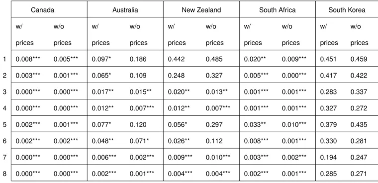
Table 1:CW p-values based on standard OLS regressions

Canada Australia New Zealand South Africa South Korea

w/ prices w/o prices w/ prices w/o prices w/ prices w/o prices w/ prices w/o prices w/ prices w/o prices 1 0.008*** 0.005*** 0.097* 0.186 0.442 0.485 0.020** 0.009*** 0.451 0.459 2 0.003*** 0.001*** 0.065* 0.109 0.248 0.327 0.005*** 0.000*** 0.417 0.422 3 0.000*** 0.000*** 0.017** 0.015** 0.020** 0.013** 0.001*** 0.001*** 0.283 0.337 4 0.000*** 0.000*** 0.012** 0.007*** 0.012** 0.007*** 0.001*** 0.001*** 0.327 0.272 5 0.002*** 0.001*** 0.077* 0.120 0.056* 0.297 0.033** 0.010*** 0.379 0.435 6 0.002*** 0.002*** 0.048** 0.071* 0.026** 0.112 0.008*** 0.001*** 0.330 0.281 7 0.000*** 0.000*** 0.006*** 0.002*** 0.009*** 0.010*** 0.003*** 0.002*** 0.194 0.247 8 0.000*** 0.000*** 0.002*** 0.001*** 0.004*** 0.004*** 0.002*** 0.001*** 0.285 0.271

8_{Just to double check, Newey-West regressions with four lags were performed for Australia’s models, which present both}

autocorrelation and heteroscedasticity problems. As it can be seen from Table 1, Appendix F, the HAC regressions have no impact on the CW statistics used to evaluate the forecasting performance of the models.

9_{Note that Stata only gives p-values for bilateral tests. To obtain the one-sided p-values listed in Table 1, the following}

(24)

Canada Australia New Zealand South Africa South Korea w/ prices w/o prices w/ prices w/o prices w/ prices w/o prices w/ prices w/o prices w/ prices w/o prices 9 0.002*** 0.006*** 0.193 0.118 0.335 0.319 0.008*** 0.001*** 0.338 0.420 10 0.001*** 0.155 0.120 0.106 0.214 0.265 0.002*** 0.013*** 0.397 0.428 11 0.000*** 0.001*** 0.013** 0.011** 0.005*** 0.004*** 0.001*** 0.002*** 0.251 0.368 12 0.000*** 0.043** 0.009*** 0.166 0.005*** 0.038** 0.002*** 0.031** 0.361 0.296 13 0.001*** 0.003*** 0.115 0.079* 0.013** 0.077* 0.011** 0.002*** 0.247 0.308 14 0.002*** 0.121 0.076* 0.083* 0.013** 0.276 0.002*** 0.010*** 0.287 0.264 15 0.001*** 0.000*** 0.004*** 0.002*** 0.002*** 0.003*** 0.001*** 0.001*** 0.194 0.266 16 0.000*** 0.024** 0.001*** 0.004*** 0.002*** 0.006*** 0.001*** 0.010*** 0.334 0.255

Note: ∗_,∗∗_{, and}∗∗∗ _{indicate that the alternative model significantly outperforms the random walk (without drift)}

at 10, 5, and 1% significance level, respectively, based on standard normal critical values for a one-sided t-test.

With commodity prices included in the regression, the results in Table 1 demonstrate that for Canada, all models outperform the random walk (without drift) at the 1% significance level. For Australia, all models outperform the random walk at either the 1, 5, and 10 % significance levels, except for models 9, 10, and 13. New Zealand’s performance is similar to that of Australia: when the three significance levels are combined, all models outperform the random walk except for models 1, 2, 9, and 10. South Africa’s models performance are similar to that of Canada: all models have significant predictive power the 10% significance level. For South Korea, none of the models forecasts better than a random walk without drift.

When the model under the null is the random walk without drift, incorporating commodity prices in the forecasting econometric equation can improve the performance of some countries’ models. Canada and New Zealand offer the strongest evidence that including commodity prices can increase the predictive power of some of the Taylor rule-based models. As we can see from table 1, Canada’s models 10 and 14 no longer outperform the random walk once oil prices are excluded from their regression. New Zealand’s models 5, 6, and 14 in addition to models 1, 2, 9, and 10 do not outperform the random walk once lamb prices are excluded from the regression. For Australia, models 1, 2, 5, and 12 does not survive the CW test once coal prices are excluded (models 9 and 10 continue to perform poorly). The only performance

(25)

that is improved once coal prices are excluded is that of model 13, which outperforms the random walk at the 10% significance level once regressions are done without coal prices. In the case of South Africa, no statistically significant differences are found once gold prices are excluded from the equations. Without gold prices, all models continue to outperform the random walk at either the 1 or 5% significance levels. South Korea’s models continue to perform worse than a random walk with overall higher p-values if oil prices are excluded.

So far in this discussion, the performance of each of the 16 models is tested when the model in the null is the random walk without drift. Now that we know which models outperform the random walk, we can answer the question, what is the improvement brought about by including commodity prices in the forecasting equation? Before I proceed to answer this question, however, it is necessary to check for serial correlations in the residuals of the regression on ˆft+1because residual serial correlations can

have an impact on the CW p-values obtained. In section 4.3.6, I return to the question of whether or not incorporating commodity prices improve the performance of the model proposed by Molodtsova and Papell (2009).

4.3.5 HAC Robust Inference

As mentioned in section 4.3.2, Clark and West (2007) advise using a robust standard error in the pres-ence of serial correlations in the residuals of the regression on ˆft+1. The residuals resulting from the

regression on ˆft+1 with commodity prices are indeed strongly autocorrelated and heteroscedastic for

almost all models. Table 2 in appendix D gives the Breusch-Godfrey and ARCH test results for all coun-tries. For Canada, all residuals are autocorrelated and all but the residuals for models 2, 6, 10 and 14, are heteroscedastic. For Australia, all models’ residuals are both autocorrelated and heteroscedastic, except for the residuals of models 9 and 13, which are only autocorrelated. All South African residuals are serially correlated but, except for model 1, none are heteroscedastic. Finally, the residuals for South Korea are all autocorrelated except for the residuals of model 7, and heteroscedastic except for the residuals of models 3 and 7.

Since the residuals resulting from the OLS regression on ˆft+1are characterised by serial correlations

and ARCH disturbances, OLS regressions with a Newey-West robust variance estimator (Newey and West, 1987) are performed. Theory dictates three options to calculate the Newey-West lag:

(26)

2. lg = f loor[P1/4]proposed by Greene (2003, p. 200)

3. lsw = f loor[0.75P1/3]proposed by Stock and Watson (2007, p. 607)

With P = 237, which is the number of forecasts performed for Canada, Australia, and South Africa, the following results are obtained: lnw = f loor[4.85], lg = f loor[3.92], lsw = f loor[4.64]. Two HAC-robust

regressions on ˆft+1with commodity prices are thus performed using Newey-West lag values of 3 and 4.

For New Zealand and South Korea, whose P = 127 and 222 respectively, the lags obtained are also 3 and 4. Note that regressions for South Korea were not performed because the models for South Korea have poor predictive performance even with standard inference.

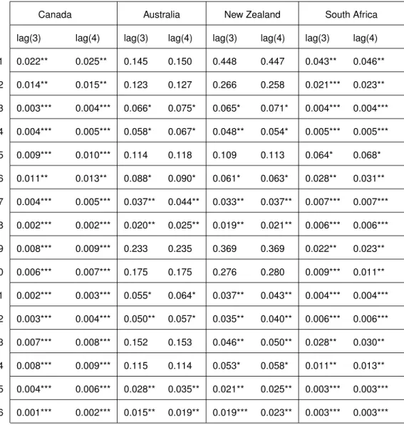
Table 2: CW p-values based on Newey-West standard errors - models with commodity prices

Canada Australia New Zealand South Africa

lag(3) lag(4) lag(3) lag(4) lag(3) lag(4) lag(3) lag(4)

1 0.022** 0.025** 0.145 0.150 0.448 0.447 0.043** 0.046** 2 0.014** 0.015** 0.123 0.127 0.266 0.258 0.021*** 0.023** 3 0.003*** 0.004*** 0.066* 0.075* 0.065* 0.071* 0.004*** 0.004*** 4 0.004*** 0.005*** 0.058* 0.067* 0.048** 0.054* 0.005*** 0.005*** 5 0.009*** 0.010*** 0.114 0.118 0.109 0.113 0.064* 0.068* 6 0.011** 0.013** 0.088* 0.090* 0.061* 0.063* 0.028** 0.031** 7 0.004*** 0.005*** 0.037** 0.044** 0.033** 0.037** 0.007*** 0.007*** 8 0.002*** 0.002*** 0.020** 0.025** 0.019** 0.021** 0.006*** 0.006*** 9 0.008*** 0.009*** 0.233 0.235 0.369 0.369 0.022** 0.023** 10 0.006*** 0.007*** 0.175 0.175 0.276 0.280 0.009*** 0.011** 11 0.002*** 0.003*** 0.055* 0.064* 0.037** 0.043** 0.004*** 0.004*** 12 0.003*** 0.004*** 0.050** 0.057* 0.035** 0.040** 0.006*** 0.006*** 13 0.007*** 0.008*** 0.152 0.153 0.046** 0.050** 0.028** 0.030** 14 0.008*** 0.009*** 0.115 0.114 0.053* 0.058* 0.011** 0.013** 15 0.004*** 0.006*** 0.028** 0.035** 0.021** 0.025** 0.003*** 0.003*** 16 0.001*** 0.002*** 0.015** 0.019** 0.019*** 0.023** 0.003*** 0.003***

(27)

Note: ∗_,∗∗_{, and}∗∗∗ _{indicate that the alternative model significantly outperforms the random walk (without drift)}

at 10, 5, and 1% significance level, respectively, based on Newey-West (1987) robust inference for a one-sided t-test.

As one can see from the table above, most models with commodity prices are non-sensitive to HAC robust-inference, specially, models for Canada and South Africa. Moreover, all countries’ models are non-sensitive to the number of lags used in the Newey-West robust-inference. In the case of Canada, all models significantly outperform the random walk model at the 1% level, with non-robust inference. Once HAC robust-inference is used, all models still outperforms the random walk model regardless of the number of lags used, although for some models the significance level is increased to 5%. Similar to Canada, South Africa’s models are insensitive to robust inference: all models continue to outperfom the random walk model at either 1, 5 or 10% significance level even with four Newey-West lags. For Australia, when non-robust inference is used, thirteen models outperform the random walk model. For significance levels of either 5 or 10%, this number reduces to nine once robust inference with either three or four Newey-West lags is used. New Zealand has twelve models with significant non-robust predictive power and eleven models with robust inference with either three or four lags.

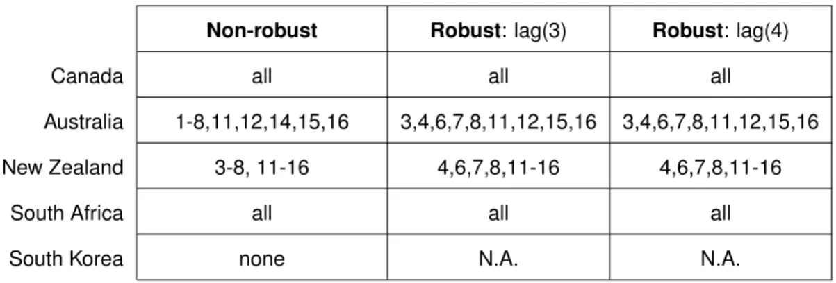
The table below summarizes which models survive the robust inference exercice for each contry, all significance levels combined.

Table 3:Models with commodity prices, robust vs. non robust inference

Non-robust Robust: lag(3) Robust: lag(4)

Canada all all all

Australia 1-8,11,12,14,15,16 3,4,6,7,8,11,12,15,16 3,4,6,7,8,11,12,15,16

New Zealand 3-8, 11-16 4,6,7,8,11-16 4,6,7,8,11-16

South Africa all all all

South Korea none N.A. N.A.

4.3.6 Forecasting with Commodity Prices

Now that we know which models with commodity prices robustly outperform the random walk, we can see if these same models forecast better than the models without commodity prices. The table below presents the test results when the model under the null is the one without commodity prices. Models for South Korea are not considered since they all failed the test against the random walk. The CW p-values

(28)

(one-sided) are obtained by regressing ˆft+1on a constant, as explained in section 4.3.2. Small p-values

mean that the null of equal predictability is rejected in favor of the alternative that models with commodity prices forecast better than models without.

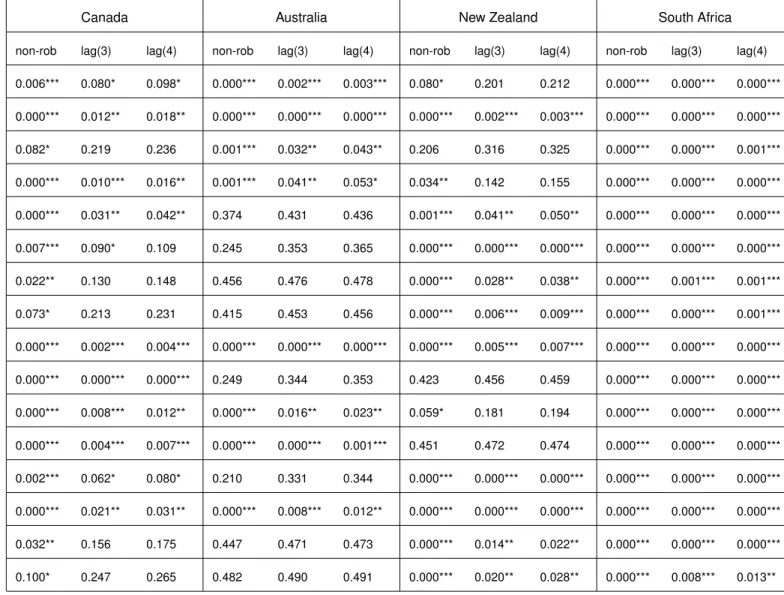
Table 4: CW p-values when the null is the model without commodity prices

Canada Australia New Zealand South Africa

non-rob lag(3) lag(4) non-rob lag(3) lag(4) non-rob lag(3) lag(4) non-rob lag(3) lag(4) 1 0.006*** 0.080* 0.098* 0.000*** 0.002*** 0.003*** 0.080* 0.201 0.212 0.000*** 0.000*** 0.000*** 2 0.000*** 0.012** 0.018** 0.000*** 0.000*** 0.000*** 0.000*** 0.002*** 0.003*** 0.000*** 0.000*** 0.000*** 3 0.082* 0.219 0.236 0.001*** 0.032** 0.043** 0.206 0.316 0.325 0.000*** 0.000*** 0.001*** 4 0.000*** 0.010*** 0.016** 0.001*** 0.041** 0.053* 0.034** 0.142 0.155 0.000*** 0.000*** 0.000*** 5 0.000*** 0.031** 0.042** 0.374 0.431 0.436 0.001*** 0.041** 0.050** 0.000*** 0.000*** 0.000*** 6 0.007*** 0.090* 0.109 0.245 0.353 0.365 0.000*** 0.000*** 0.000*** 0.000*** 0.000*** 0.000*** 7 0.022** 0.130 0.148 0.456 0.476 0.478 0.000*** 0.028** 0.038** 0.000*** 0.001*** 0.001*** 8 0.073* 0.213 0.231 0.415 0.453 0.456 0.000*** 0.006*** 0.009*** 0.000*** 0.000*** 0.001*** 9 0.000*** 0.002*** 0.004*** 0.000*** 0.000*** 0.000*** 0.000*** 0.005*** 0.007*** 0.000*** 0.000*** 0.000*** 10 0.000*** 0.000*** 0.000*** 0.249 0.344 0.353 0.423 0.456 0.459 0.000*** 0.000*** 0.000*** 11 0.000*** 0.008*** 0.012** 0.000*** 0.016** 0.023** 0.059* 0.181 0.194 0.000*** 0.000*** 0.000*** 12 0.000*** 0.004*** 0.007*** 0.000*** 0.000*** 0.001*** 0.451 0.472 0.474 0.000*** 0.000*** 0.000*** 13 0.002*** 0.062* 0.080* 0.210 0.331 0.344 0.000*** 0.000*** 0.000*** 0.000*** 0.000*** 0.000*** 14 0.000*** 0.021** 0.031** 0.000*** 0.008*** 0.012** 0.000*** 0.000*** 0.000*** 0.000*** 0.000*** 0.000*** 15 0.032** 0.156 0.175 0.447 0.471 0.473 0.000*** 0.014** 0.022** 0.000*** 0.000*** 0.000*** 16 0.100* 0.247 0.265 0.482 0.490 0.491 0.000*** 0.020** 0.028** 0.000*** 0.008*** 0.013**

Note: ∗_,∗∗_{, and}∗∗∗ _{indicate that models with commodity price significantly outperforms the ones without at the}

10, 5, and 1% significance level, respectively, based on critical values (robust in the case of columnsLAG(3)

andLAG(4)) for a one-sided t-test.

As it can been seen from tables 3 and 4, South Africa and Canada present the best evidence that models with commodity prices outperforms both the random walk and models without commodity prices. In the case of South Africa all models pass the double test even when four Newey-West lags are used. For Canada, ten models outperform both the random walk and the forecast without commodity prices.

(29)

Australia and New Zealand present less evidence that commodity prices improve the performance of the Taylor rule-based forecasting equation. Only four Australian models and seven New Zealand models pass the double test. The models for each country that pass the double test are:

• Canada: 1, 2, 4, 5, 9, 10, 11, 12, 13 ,14 • Australia: 3, 4, 11, 12

• New Zealand: 6, 7, 8, 13, 14, 15, 16 • South Africa: all

4.3.7 Model choice

Two criterias can be used in order to choose among the surviving models listed in the previous section. The first criteria is to choose those models that outperforms models without commodity prices with the lowest p-values. Using this criteria, and choosing robust inference with four lags, the best models for Canada would be models 9, 10, and 12, whose results are all significant at the 1% level. For Australia, the chosen models would be models 3, 11, and 12, which have results significant at either the 5 or 1%. In the case of New Zealand, at the 1% significance level, the models would be 6, 8, 13, and 14. Note that for Australia and New Zealand, the chosen models outperform the random walk only at the 5 or 10% significance level. Finally, this criteria does not apply so well for South Africa because all South African models outperform both the random walk and the models without commodity prices at the 1% significance level.

A second criteria is thus necessary for South Africa. Such a criteria could be choosing the models that are most parsimonious. Models 9 and 10 would then be the best, with Model 10 being the most parsimonious because it is symmetric with no smoothing, have homogeneous coefficients, and is without a constant. Model 9 is similar except that it includes a constant. One could also use the R-squared values to see which models fit the data the best. Referring to the R-squared values provided in table 2 in appendix F, the highest R-squared values are for models 16 and 8: 0.0762 and 0.0812, respectively.

5 Conclusion

The objective of this research project is to verify whether including commodity prices improves the fore-casting performance of the econometric model proposed by Molodtsova and Papell (2009) for Canada,

(30)

Australia, New Zealand, South Africa and South Korea. The answer is affirmative for Canada, Australia, New Zealand and South Africa, although there are differences in performance according to the model specification. The best evidence is given by Canada and South Africa and the worst is by South Korea because South Korean’s models do not outperform the random walk, regardless of the specification. The reason for the poor perfomance of the South Korean models could be either because South Korea do not have a de-facto flexible exchange rate regime or because South Korea’s central bank do not follow the Taylor rule when setting its monetary policy.

(31)

REFERENCES

Amano, Robert A., and Simon Van Norden. 1993. Terms of trade and real exchange rates: the Canadian evidence. Bank of Canada.

Amano, Robert A., and Simon Van Norden. 1998. Exchange Rates and Oil Prices. Review of International Economics 6: 683-694.

Clarida, Richard, Jordi Gall and Mark Gertler. 1999. The Science of Monetary Policy: A New Keynesian Perspective. Journal of Economic Literature 37: 1661-1707.

Clark, Todd .E., and Kenneth D. West. 2006. Using out-of-sample mean squared prediction errors to test the martingale difference hypothesis. Journal of Econometrics 135: 155-186.

Clark, Todd .E., and Kenneth D. West. 2007. Approximately normal tests for equal predictive accuracy in nested models. Journal of Econometrics 138: 291-311.

Chen, Yu-chin, and Kenneth Rogoff. 2003. Commodity Currencies. Journal of International Economics 60: 133-160.

Chen, Yu-chin. 2004. Exchange rates and fundamentals: Evidence from commodity economies. University of Washington.

Diebold, Francis X., and Roberto S. Mariano. 1995. Comparing predictive accuracy. Journal of Business and Economic Statistics 13: 253-263.

Dornbusch, Rudiger. 1976. Expectations and Exchange Rate Dynamics. Journal of Political Economy 84: 1161-1176

Gourinchas, Pierre-Olivier and Aaron Tornell. 2004. Exchange rate puzzles and distorted beliefs. Journal of International Economics 64: 303-333.

Greene, William H. 2003. Econometric analysis. 5th ed. New Jersey: Prentice Hall.

Hansen, Bruce E. 1992. Test for parameter Instability in Regressions with I(1) processes. Journal of Business and Economic Statistics 10: 321-335.

Hansen, Peter R. 2005. A test for superior predictive ability. Journal of Business and Economic Statistics 23: 365-380.

Lafrance, Robert and Simon van Norden. 1995. Exchange rate fundamentals and the Canadian dollar. Bank of Canada Review. Spring issue: 17-33.

Lardic, Sandrine and Valérie Mignon. 2002. Économétrie des séries temporelles macroéconomiques et financières. Paris: Economica.

Meese, Richard A., and Kenneth Rogoff. 1983. Empirical Exchange Rate Models of the Seventies: Do they fit out of sample? Journal of International Economics 14: 3-24.

(32)

Taylor Rule Fundamentals. Journal of International Economics 77: 137-276.

Newey, Whitney K. and Kenneth D. West. 1987. A Simple, Positive Semi-definite, Heteroskedasticity and Autocorrelation Consistent Covariance Matrix. Econometrica 55 (issue 3): 703-708

Stock, James H. and Mark W. Watson. 2007. Introduction to econometrics. 2nd ed. Boston: Pearson Education.

West, Kenneth D. 1996. Asymptotic inference about predictive ability. Econometrica 64: 1067-1084. Wooldridge, Jeffrey M. 2009. Introductory Econometrics: A Modern Approach. 4th ed. Mason: South-

(33)