CAHIER 06-2002
SOME IMPLICATIONS OF THE ZERO LOWER BOUND ON INTEREST RATES FOR THE TERM STRUCTURE AND MONETARY POLICY
CAHIER 06-2002
SOME IMPLICATIONS OF THE ZERO LOWER BOUND ON INTEREST RATES FOR THE
TERM STRUCTURE AND MONETARY POLICY
Francisco J. RUGE-MURCIA1
1 Centre de recherche et développement en économique (C.R.D.E.) / Centre interuniversitaire
de recherche en économie quantitative (CIREQ) and Département de sciences économiques, Université de Montréal
May 2002
_______________________
This project was started while the author was visiting scholar at the Research Department of the International Monetary Fund. He is grateful to the IMF for its hospitality and to its staff for their help collecting the data. The author wishes to thank Rui Castro for helpful discussions. Financial support from the Social Sciences and Humanities Research Council of Canada and the Fonds pour la formation de chercheurs et l’aide à la recherche of Québec is gratefully acknowledged.
RÉSUMÉ
Dans une économie sans taux de dépréciation monétaire (en terme réel), le taux d’intérêt nominal est positif ou nul. Ce papier tire les implications de cette contrainte de non-négativité pour la structure à terme et montre qu’il induit une relation non linéaire et convexe entre le taux d’intérêt de court et de long terme. Par conséquent, le taux de long terme répond de façon asymétrique aux changements dans le taux de court terme et a une valeur plus petite que celle prédite par un modèle linéaire de base. En particulier, une baisse du taux d’intérêt de court terme conduit à une baisse du taux d’intérêt de long terme plus petite (en valeur absolue) que l’augmentation du taux d’intérêt de long terme associée à une augmentation du taux de court terme de même grandeur. Dans la mesure où la politique monétaire agit en affectant les taux de long terme à travers la structure à terme, sa puissance est considérablement réduite aux bas taux d’intérêts. Les prédictions empiriques du modèle sont examinées en utilisant les données du Japon.
Mots clés : modèles limités dépendants avec anticipations rationnelles, prévision non linéaire, politique monétaire, Japon
ABSTRACT
In an economy where cash can be stored costlessly (in nominal terms), the nominal interest rate is bounded below by zero. This paper derives the implications of this nonnegativity constraint for the term structure and shows that it induces a nonlinear and convex relation between short- and term interest rates. As a result, the long-term rate responds asymmetrically to changes in the short-long-term rate, and by less than predicted by a benchmark linear model. In particular, a decrease in the short-term rate leads to a decrease in the long-term rate that is smaller in magnitude than the increase in the long-term rate associated with an increase in the short-term rate of the same size. Up to the extent that monetary policy acts by affecting long-term rates through the term structure, its power is considerably reduced at low interest rates. The empirical predictions of the model are examined using data from Japan.
Key words : limited-dependent rational-expectations models, nonlinear forecasting, monetary policy, Japan
1
Introduction
In an economy where cash can be stored costlessly, the nominal interest rate is bounded by below zero. Fisher (1896, p. 31) argues that arbitrage insures nonnegative nominal interest rates because agents would rather hoard the currency, rather than lend it at a loss. McCallum (2000) constructs a general equilibrium model where money facilitates transactions. If the marginal benefit of holding real money balances is decreasing but strictly positive, the nominal interest rate is always positive. If there is a quantity beyond which additional real money balances provide no extra services, agents are satiated with money and the nominal interest rate is zero. Hence, the values that the nominal interest rate can take are limited to the interval [0,∞).
The notion of a zero lower bound on interest rates rests on the assumption that money can be stored without cost. Fisher (1896, p. 32) points out that if money were a perishable commodity, the lower bound on the nominal interest rate would be negative. Even if currency is not perishable, Thornton (1999) and McCallum (2000) argue that storing safely large amounts of currency is costly. Consequently, individuals might be willing to hold financial assets that promise a negative nominal return. Thornton suggests that in this case the negative return represents a fee paid to the bond issuer by the bearer in exchange for storage services. Cecchetti (1988) shows that the observation of negatives interest rates in the United States during and following the Great Depression is due to the “exchange privilege.” The exchange privilege gave current holders of Treasury securities the right to buy new securities on a future date. Once the exchange privilege is priced appropriately, the corrected yields are strictly positive and bounded below by zero.
When the nominal interest rate is zero, money and bonds are perfect substitutes. The economy is in a liquidity trap where individuals are prepared to hold any amount of money supplied. Thus, increases in the money supply through open market operations have no effect on the interest rate or income. Monetary policy when the nominal interest rates are bounded below by zero has been studied by Fuhrer and Madigan (1997), Orphanides and Wieland, (1998), Wolman (1998), Woodford (1999), and McCallum (2000). The goal of this paper is more modest and slightly different. This paper zooms in a particular channel for the transmission of monetary policy, namely the term structure of interest rates, and derives the time-series implications of the zero lower bound for long-term interest rates under the Pure Expectations Hypothesis (PEH). It is shown that the zero lower bound induces a nonlinear and convex relation between the long-term interest rate and the level and standard deviation of the short-term interest rate. As a result, the response of long-term interest rates to changes in the short-term interest rate is asymmetric and smaller than predicted by a linear
forecasting model. A decrease in the short-term rate leads to a decrease in the long-term rate that is smaller in magnitude than the increase in the long-term rate associated with an increase in the short-term rate of the same size. In both the linear and nonlinear forecasting models, the effect on the long-term interest rate decreases with the horizon but it is more severe for the nonlinear model. Up to the extent that monetary policy acts by affecting long-term rates through the term structure, its power is considerably reduced at low interest rates.
The zero lower bound on interest rates is imposed by assuming that the short-term nominal interest rate is a limited-dependent variable. This specification is based on the interpretation of interest rates as options in Black (1995). The limited-dependent variable model is a device that forces agents to consider explicitly the zero lower bound when con-structing their forecasts, even if all observations of the nominal interest rate to date are strictly positive. In general, deriving the conditional expectations of this nonlinear process is nontrivial. However, for the simple case of a two-period bond and normally distributed disturbances, it is possible to derive closed-form analytical results. For longer horizons and more general distributional assumptions, there is no closed-form expression for the condi-tional expectation of the short-term interest rate. In order to address this problem, this paper proposes a frequency simulator to compute numerically the conditional expectations. Using Monte-Carlo experiments, it is shown that the simulator delivers numerically exact es-timates of the conditional expectations and that antithetic variates can reduce substantially the variance of the forecast estimator.
The model is calibrated using weekly Japanese data. The comparison of the nonlinear and a linear forecasting models indicates that the former yields smaller forecasts errors than the latter. This is basically due to the fact that the nonlinear model predicts more accurately the slope of the term structure at very low interest rates. Black (1995, p. 1373) argues that option pricing considerations imply that the long-term interest rate should rise with the volatility of the short-term rate. However, results indicate that volatility effect described by Black is likely of play a minor role in the determination of the Japanese long-term interest rates.
The paper is organized as follows. Section 2 develops some intuition regarding the source of the zero lower bound using a simple general equilibrium model, and motivates the limited-dependent variable model for the short-term interest used thereafter. Section 3 introduces a simple time-series process for the one-period bond that describes the fact that interest rates are bounded below by zero and derives the implications of the nonlinear model for a two-period bond when shocks are normally distributed. Section 4 derives the conditional expectations for longer horizons and under general distributional assumption. Section 5
proposes a frequency simulator and provides Monte-Carlo evidence on its accuracy. Section 6 calibrates the model for the term structure using data from Japan. Section 7 concludes.
2
A Simple General Equilibrium Model
This section constructs a simple general equilibrium model that (i) develops some intuition regarding the zero-lower bound on interest rates and (ii) motivates the limited-dependent variable model employed in Sections 3 and 4. This general equilibrium model is close in spirit to Wolman (1998) and McCallum (2000). The economy consists of an infinitely-lived representative agent that supplies labor inelastically, a representative firm, and a government. There is no population growth. The population size is normalized to one. The single good is produced by perfectly competitive firms using the technology: yt = ztg(kt), where
yt is output, zt is a stationary technology shock, kt is capital per capita, and g(·) is a
production function that satisfies the Inada conditions. For simplicity, it is assumed that the depreciation rate is zero. Taking the good a numeraire, profit maximizing implies that the real rental price of capital equals the marginal product of capital.
The representative agent choose sequences of consumption and holdings of money, capital, and bonds to maximize:
Et ∞
X
s=t
ρs−t[U (cs) + V (ms)], (1)
where ρ ∈ (0, 1) is the subjective discount factor, ct is consumption, mt is real money
balances, and U (·) and V (·) are increasing and concave functions of their arguments. U(·) satisfies the Inada conditions. The marginal utility of money tends to infinity when m tends to zero, but it is possible that there exists a level of m, say ¯m > 0, for which agents are satiated with money in the sense that V0(m) = 0 for any m > ¯m. Nominal risk-free
government bonds of different maturities n = 1, 2, . . . , N are available. The return at time t on the one-period nominal bond contracted at time t− 1 is denoted by rt. The return
at time t on the n-period nominal bond contracted at time t− n is denoted by Rt(n). The
agent’s resources at time t are the wage and rent received from selling labor and renting capital to firms, money holdings set aside in period t− 1, principal and returns from past bond investments, and lump-sum transfers (net of taxes) from the government. Utility maximization is subject to the budget constraint (expressed in real terms):
ct+ (kt+1− kt) + mt+ N P n=1 b(n)t = g(kt) + mt−1/(1 + πt) + (1 + rt)b (1) t−1/(1 + πt) + N P n=2 h (1 + R(n)t )b(n)t−n/Qn−1i=0(1 + πt−i)i+ τt,
where b(n)t are the amount of bonds with maturity n purchased at time t, πt is the rate of
inflation between time t− 1 and t, and τt is transfers. First-order necessary conditions
for utility maximization imply that the expected real return on capital, bonds of different maturities and money should be all equal at the optimum.
The government finances transfers and redeems maturing debt by raising seigniorage and issuing new debt subject to the no-Ponzi-game condition. In every period:
N X n=1 b(n)t +(mt−mt−1/(1+πt)) = τt+(1+rt)b (1) t−1/(1+πt)+ N X n=2 · (1 + R(n)t )b (n) t−n/ n−1Q i=0 (1 + πt−i) ¸ . One could interpret monetary policy as determining the rate of growth of the nominal money supply: Mt= (1 + µ)Mt−1. In real terms, this process implies mtπt = µmt−1.
Consider the (deterministic) steady state of this system:
π = µ, (2)
V0(m)/U0(c) = r/(1 + r), (3)
1 + g0(k) = 1/ρ, (4)
1 + r = (1 + π)/ρ, (5)
1 + R(n) = (1 + r)n. (6)
Equation (2) states that, in the steady state, inflation equals the rate of nominal money growth. Equation (3) defines the demand for real balances. Equation (4) determines the real interest rate as function of the agent’s subjective discount factor. Equation (5) is the Fisher equation for the one-period nominal interest rate. Equation (6) is a term-structure relation that determines the return on the long-term bond as a function of the compounded return on the one-period bond.
Friedman’s Rule is obtained by setting µ = ρ− 1. Substituting Friedman’s Rule into (5) implies that the (steady-state) nominal interest rate is zero. Equation (3) then implies that V0(m) = 0 meaning that at this rate of money growth, agents must be satiated with money.
The following proposition shows that it is not possible to implement a monetary policy rule with a rate of money growth lower than Friedman’s Rule. Consequently, zero is the lower bound on the nominal interest rate.
Proposition 1. Zero Lower-Bound on the Nominal Interest Rate. If the marginal utility of real money balances is nonnegative, then it is not possible to implement a monetary policy with µ < ρ− 1, and the nominal interest rate is bounded below by zero.
Proof. The proof is by contradiction. Assume that µ < ρ− 1. Then, π < ρ − 1 and, by equation (5), r < 0. However, by equation (3), r> 0. For the second part of the proposition, note that since µ> ρ − 1, then π > ρ − 1 and, by equation (5), it follows that r > 0.
In this general equilibrium model, the condition that insures the nonnegativity of the nominal interest rate is the assumption that the marginal utility of money is nonzero. Wol-man (1998) and McCallum (2000) construct shopping-time models where money reduces the time or cost involved in making transactions. In their case, the assumption that the trans-action function is decreasing in the level of real money balances (up to a satiation point) insures that nominal interest rate is bounded below by zero. Fisher (1896, p. 31) argues that arbitrage insures nonnegative nominal interest rates because agents would rather hoard the unit of exchange, rather than lend it at a loss. The critical assumption in all cases, is that money can be stored without cost. Provided this assumption is satisfied, the range of values that the nominal interest rate can take is the interval [0,∞).1
3
The Two-Period Bond
This section introduces a simple time-series model for the one-period nominal interest rate that represents the idea that nominal interest rates are bounded below by zero. This section then derives the implications of this nonnegativity constraint for a long-term bond with maturity equal to two periods. Considering this special case first is instructive because under certain conditions, one can write a closed-form expression linking the short- and long-term interest rates and derive analytically the implications of the zero lower bound.
The model for the one-period nominal interest rate is based on the discussion by Black (1995). Black proposes a characterization of the short-term interest rate that distinguishes between the observed and the shadow nominal interest rates. The observed nominal interest rate is bounded below by zero because agents can hold money without cost. The shadow nominal interest rate can be positive or negative, reflecting completely the expected rates of inflation and real return.2 The observed and shadow interest rates are related by:
rt= max(rt∗, 0), (7)
where rtand r∗t are the one-period observed and shadow nominal interest rates, respectively.
Equation (7) is exactly equivalent to:
1Whether zero itself is included in the interval depends on whether there is a level of real balances for
which agents are satiated with money. If the marginal utility of money is strictly positive, then r ∈ (0, ∞).
2Black (p. 1372) argues that currency is an option in the sense that were the bond return negative, agents
could hold currency instead. Alternatively, one can interpret rt as an option on r∗t with a strike price of
zero, where r∗
t is what the interest rate would be in the absence of the currency option. This is the “shadow”
interest rate. Cox, Ingersoll, and Ross (1985) construct a model of the term structure where the process of the short-term interest rate is specified in logs. As a result, the short-term interest rate is bounded below by zero.
rt=
½ r∗
t, if r∗t > 0,
0, otherwise. (8)
Under (8), the observed nominal interest rate could be interpreted as a limited-dependent variable censored at zero, with r∗
t as associated latent variable. A model of this form was
first studied in a regression context by Tobin (1958) and is a standard tool in cross-section econometrics. The use of limited dependent variable models in a time-series framework is usually more complicated because economic models frequently predict that expectations is one of the explanatory variables. Limited-dependent models with rational expectations have been employed, for example, by Shonkwiler and Maddala (1985), and Holt and Johnson (1989) to study the determination of commodity prices in price-support schemes, by Baxter (1990) to study adjustable-peg exchange rate regimes, and by Pesaran and Samiei (1992, 1995) and Pesaran and Ruge-Murcia (1999) to study exchange rates subject to two-sided limits.
By the Pure Expectations Hypothesis (PEH) of the term structure of interest rates, the nominal return on a two-period zero-coupon bond must equal the average expected return on the sequence of two one-period bonds held over its lifetime:
Rt= (1/2) [rt+ E(rt+1|It)] + θt, (9)
where Rt is the return on the two-period bond, It is the nondecreasing set of information
available to market participants at time t and is assumed to include observations of the variables up to and including period t, E(rt+1|It) is the conditional expectation of the nominal
return on the one-period bond acquired at time t + 1, and θt is a serially uncorrelated
stochastic term that includes a liquidity premium and has variance σθ2.
In order to give empirical content to the theory, it is necessary to specify a process for the shadow nominal interest rate. Let us assume that r∗
t is generated by:
r∗t = α + ψ(L)rt+ βxt+ ²t, (10)
where α is an intercept, L is the lag operator, ψ(L) stands for the polynomial
p
P
j=1
ψjLj, β
is a 1× m vector of parameters, xt is a m× 1 vector of explanatory variables, and ²t is a
disturbance term with zero mean and variance σ2
², serially uncorrelated, and uncorrelated
with θt. The unconditional variance of ²t is constant, but its conditional variance could
be time-varying. For example, the conditional variance of ²t could be described by an
ARCH-type model [Engle (1982)] in order to capture the observed changes in volatility in short-term interest rates. The process (10) does not pretend to be a structural representation
and simply describes the statistical projection of the latent nominal interest rate on a subset of the variables by which it is actually determined. Wolman (1998) considers a deterministic version of (8)-(10) where r∗
t is the central bank’s desired short-term nominal interest rate
and arises from a Taylor-type policy rule.
The explanatory variables in xt could be generated by the linear stochastic process:
xt = AHt−1+ w1,t, (11)
where A is a m× b matrix of coefficients, Ht is a b× 1 vector of predetermined variables
possibly including past values of xt, and w1,t is a m× 1 vector of random disturbances
assumed independently and identically distributed (i.i.d.) (0,Ω1/2) and uncorrelated with θ t
and ²t.
Since the process of the short-term nominal interest rate is nonlinear, the construction of the conditional expectation, E(rt+1|It), that enters (9) is not obvious. A case where it
is possible to find a closed-form expression for this conditional expectation is the one where shocks are normally distributed. In addition, it is easiest to see the relation between the short- and the long-term interest rates when one assumes that r∗
t depends only on the first
lag of rt :
r∗t = α + ψrt−1+ ²t, (12)
with ²t ∼ N(0, σ2²). Since the nominal interest rate is positively autocorrelated and must
have a nonnegative unconditional mean, plausible values for α and ψ are α≥ 0 and ψ > 0. The only crucial assumption is the one of normality, remaining assumptions are not restrictive and could be relaxed if desired. Section 5 uses stochastic simulation to show that the analytical results derived below hold more generally.
The closed-form expression for E(rt+1|It) is given in the following proposition:
Proposition 2. Assume that the short-term interest rate follows the limited-dependent pro-cess (8) where r∗
t is determined according to (12). Define the variable ct+1=−E(r∗t+1|It)/σ² =
−(α + ψrt)/σ². Then, the conditional expectation of the short-term nominal interest rate at
time t + 1 constructed at time t is given by
E(rt+1|It) = (α + ψrt)[1− Φ(ct+1)] + σ²φ(ct+1), (13)
where Φ(·) and φ(·) denote the cumulative and density functions of a standard normal vari-able, respectively.
Proof. See Appendix A.
The one-step-ahead conditional expectation is a nonlinear function of the current short-term interest rate as a result of the nonnegativity constraint. This follows from the fact that
Φ(ct+1) and φ(ct+1) are nonlinear functions of ct+1, that in turn is a function of rt. Taking
the first and second derivatives of E(rt+1|It) with respect to rt yields ∂E(rt+1|It)/∂rt =
ψ[1− Φ(ct+1)], and ∂2E(rt+1|It)/∂rt2 = (ψ2/σ²)φ(ct+1) > 0. Thus, E(rt+1|It) is increasing on
rt in the plausible case where ψ > 0, and convex on rt for any ψ 6= 0. Notice that, provided
α > 0, the forecast is strictly positive even if the current short-term interest rate is zero. When rt = 0, the future short-term rate can only take values equal to or larger than the
current rate. Thus, the conditional expectation of rt+1 is strictly positive. As the nominal
interest rate rises above the zero lower bound, ct+1 decreases, the terms Φ(ct+1) and φ(ct+1)
tend to zero, and the model approaches a linear forecasting model (see below). Substituting (13) into the term-structure relation, (9), yields
Rt= α/2 + (1/2)(1 + ψ)rt− (1/2)(α + ψrt)Φ(ct+1) + (σ²/2)φ(ct+1) + θt. (14)
As a result of the effect of the zero lower bound on expectations, the return on the two-period bond is related nonlinearly to the one-two-period return. A simple way to characterize this relation is to take the first and second derivative of Rt with respect to rt:
∂Rt/∂rt = 1/2 + (ψ/2)[1− Φ(ct+1)],
and
∂2Rt/∂r2t = (ψ 2/2σ
²)φ(ct+1) > 0.
Hence, the long-term interest rate is increasing on rt in the plausible case where ψ > 0, and
convex on rt for any ψ6= 0.
Because the relation between Rtand rtis nonlinear, changes in rtcan produce asymmetric
movements in the long-term rate. In particular, in the case where ψ > 0, an increase in the short-term interest rate leads an increase in the long-term rate that is larger in magnitude than the decrease in the long-term rate associated with a decrease in the short-term rate of the same size. That is,
|Rt(rt+ ∆)− Rt(rt)| > |Rt(rt− ∆) − Rt(rt)|,
where ∆ is the change in the short-term interest rate. To verify this claim, simply use ∂Rt/∂rt > 0, and the definition of absolute value to write Rt(rt+ ∆)− Rt(rt) >−[Rt(rt−
∆)− Rt(rt)]. Rearranging yields [Rt(rt+ ∆) + Rt(rt− ∆)]/2 > Rt(rt), that holds because
the function Rt(rt) is convex on its argument.
The nonlinear model also predicts that, given the current short-term interest rate, the long-term rate is an increasing and convex function of the conditional standard deviation of rt. To see this, simply take the first and second derivative of Rt with respect to σ² to
obtain ∂Rt/∂σ² = φ(ct+1)/2 > 0, and ∂2Rt/∂σ2² = c2t+1φ(ct+1)/2σ² > 0. Under Black’s
interpretation of interest rates as options, this is the result that option pricing theory would predict. The following proposition summarizes the implications of the zero lower bound for the return on the two-period bond.
Proposition 3. Assume that the one-period interest rate follows the limited-dependent process (8) where rt∗ is determined according to (12). Then, under the PEH, the two-period
interest rate is: (i) nonlinear and convex on rt for any ψ 6= 0, (ii) increasing and convex
on the conditional standard deviation of rt for any ψ6= 0, and (iii) increasing on rt for any
ψ > 0. Also, (iv) provided ψ > 0, an increase in rt leads an increase in the long-term rate
that is larger in magnitude than the decrease in the long-term rate associated with a decrease in rt of the same size.
It is interesting to compare the predictions of the nonlinear model with the ones of a benchmark linear forecasting model. The counterpart of the process (8)-(12) when one ignores the zero lower bound on interest rates is:
rt= α + ψrt−1+ ²t.
In this case, E(rt+1|It) = (α + ψrt) and
Rt = α/2 + (1/2)(1 + ψ)rt+ θt.
The process of the two-period bond is linear in rt and differs from the one in (14) by
the last two nonlinear terms that capture the effect of the nonnegativity constraint on the expectations of rt+1. Because ∂Rt/∂rt = (1 + ψ)/2 is constant and independent of the
short-term rate, changes in rt produce movements in the long-term rate that are symmetric,
proportional, and history-independent. That is, the effect on Rt of a 1 point increase in
rt is the mirror image of a 1 point decrease, one-half the effect of a 2 point increase, and
independent of the level of the short-term interest rate when the change takes place. The long-term rate is independent of the conditional standard deviation of the short-term rate. To see this, simply take ∂Rt/∂σ²= 0. Comparing the effect on Rt of a change in rtimplied
by both models, note that
1/2 + (ψ/2)[1− Φ(ct+1)] < (1 + ψ)/2.
Thus, at low interest rates the impact of adjustments to the short-term rate on the long-term rate is dampened by the effect of the nonnegativity constraint.
4
The Multi-Period Bond
Consider now the more general case where the long-term bond has maturity of n periods. The PEH predicts that the return on the n-period pure-discount bond must equal the average expected return on the sequence of n one-period bonds held over its lifetime:
Rt = (1/n) [rt+ E(rt+1|It) +· · · + E(rt+n−1|It)] + θt, (15)
where Rt is now the nominal return on the n-period bond, E(rt+s|It) is the conditional
expectation of the nominal return on the one-period bond acquired at time t + s for s = 1, 2, . . . , n− 1, and remaining notation is as previously defined.
Proposition 4 derives the conditional expectations of the short-term interest rate when rt is subject to the nonnegativity constraint. This proposition generalizes Proposition 2 in
that it makes no assumptions regarding the distributions of the shocks, uses the multivariate process (10) for r∗t, and considers horizons s≥ 1.
Proposition 4. Assume that the short-term interest rate follows the limited-dependent process (8) where r∗
t is determined according to (10). Assume that the explanatory variables,
xt, follow the process (11). Define the composite error term
us,t+s = ²t+s+ s−1
X
k=1
ψs−kµk,t+k+ βws,t+s, (16)
where µk,t+k= rt+k− E(rt+k|It) and ws,t+s = xt+s− E(xt+s|It), with cumulative distribution
and density functions denoted by Fs(·) and fs(·), respectively. Define the variable
ct+s =−E(rt+s∗ |It), (17) where E(rt+s∗ |It) = α + min{p,s−1}X k=1 ψkE(rt+s−k|It) + p X j=s ψjLjrt+s+ βE(xt+s|It). (18)
Then, the conditional expectation of the short-term nominal interest rate at time t + s con-structed at time t is given by
E(rt+s|It) =
£
E(rt+s∗ |It) + E(us,t+s|It, us,t+s > ct+s)
¤
[1− Fs(ct+s)] . (19)
Proof. See Appendix B.
For the reasons to be made clear below, the conditional expectation E(rt+s|It) cannot
of current and past realizations of the short-term interest rate. This follows from the observation that E(us,t+s|It, us,t+s > ct+s) and Fs(ct+s) are nonlinear functions of ct+s, that
in turn is a function of current and past realizations of rt. Moreover, since the long-term
interest rate depends on the average forecast of future short-term rates, Rt should also be a
nonlinear function of current and lagged short-term interest rates.
For the horizon s = 1, the forecast error rt− E(rt|It) is zero because rt forms part of
the information set at time t. Then, u1,t+1= ²t+1+ βw1,t+1 and the cumulative and density
functions of u1,t+1follow from the ones assumed for ²t+1and w1,t+1. When these disturbances
are assumed normally distributed, the one-step-ahead conditional expectation can be found analytically using results for censored normal variables [see Maddala (1983, p. 366)]:
E(rt+1|It) = E(r∗t+1|It) [1− F1(ct+1)] + f1(ct+1), (20)
where F1 and f1 correspond (respectively) to the cumulative and density functions of a
normal variable with zero mean and variance σ2
² + β0Ωβ.
For horizons s > 1, us,t+sincludes as components interest-rate forecast errors that, due to
the nonlinear nature of rt, do not follow a standard distribution. As an illustration, Figure
1 plots the density of one-step-ahead forecast errors for a specific numerical example.3 The realizations of the forecast error were constructed as follows. Taking as given the current short-term interest rate, 50000 realizations of rt+1 were generated using (8) and (12) with
α = 0.025, ψ = 0.95, and ²t ∼ i.i.d.N(0, 0.82). The nonnegativity constraint was enforced
numerically by substituting negative realization of rt+1 with zeroes. The one-step-ahead
forecast, E(rt+1|It), was obtained using the analytical expression for normal disturbances
(20). Forecasts errors were then computed as µ1,t+1 = rt+1 − E(rt+1|It). Figures 1(A)
and 1(B) assume a current short-term interest rate of 0.5 and 1.0, respectively. Although the shock to the short-term interest rate (²t) is normally distributed, the density of the
errors associated with forecasting rt+1 is nonnormal and asymmetric. The asymmetry arises
because at low interest rates, forecast errors are bounded below by −E(rt+1|It). This
asymmetry tends to disappear as the current short-term rate rises away from zero and the effect of the nonnegativity constraint diminishes. For sufficiently large values of the current short-term rate, µ1,t+1 → ²t∼ i.i.d.N(0, 0.82).
Since at low interest rates, the density of the forecast errors depends on rt, the forecast
horizon, and the model parameters, an analytical description of the density of us,t+s appears
unfeasible. Moreover, while expectations of µk,t+k conditional on It are zero, (19) involves
the more complicated conditional expectations of their truncated linear combination defined
in (16). This means that there is no closed-form expression to describe E(rt+s|It) and,
con-sequently, it is not possible to derive general analytical results. However, given a parametric process for the short-term interest rate, rt, it is possible to derive the implications of the zero
lower bound for long-term interest rates if one devises a procedure to compute numerically the conditional forecasts E(rt+s|It) for s = 1, 2, . . . , n− 1.
5
A Method to Compute the Conditional Expectations
5.1
The Procedure
This section proposes a simulation procedure to compute numerically the conditional expec-tations that enter the term structure. This procedure extends the frequency simulators by Lerman and Manski (1981) and McFadden (1989) to dynamic nonlinear rational-expectations models. Lerman and Manski, and McFadden are concerned with the estimation of the multinomial probit model. For this model, one must estimate as many recursive integrals as choices are allowed and no closed-form solution is available. Lerman and Manski draw realizations from a multivariate normal distribution and record the frequency with which utility is maximized at each alternative. The estimated probability that the decision maker selects the alternative i is the fraction of times that utility is maximized by choosing i.
For the problem here, (19) characterizes analytically the conditional expectations of rt+s
but there are no closed-form expressions for Fs(ct+s) and E(us,t+s|It, us,t+s > ct+s). The
proposed procedure constructs estimates of their magnitudes by simulating paths of the short-term nominal interest subject to the nonnegativity constraint, and computing the relative frequency with which the zero lower bound is hit and the sample average of the realizations of the nominal rate above the bound. The application of this procedure in a dynamic setup might appear computationally demanding. However, as we will see below, its application is facilitated by the observation that all conditional expectations involved in the term structure can be found recursively using the law of iterated projections.4
The simulation procedure involves the following steps.
Step 1: having found analytically or numerically (see below), the one-step-ahead conditional expectation of the nominal interest rate, E(rt+1|It), use the definitions (18) and (17) for
s = 2 to obtain ct+2.
4In previous work [see Ruge-Murcia (2000)], I have used successfully a version of this procedure for the case
where the variable of interest follows a two-sided switching regression. This paper extends the procedure to limited-dependent variable models, allows conditionally heteroskedastic disturbances, and provides Monte-Carlo evidence on the accuracy of the proposed simulation method.
Step 2: simulate M observations of the short-term interest rate at time t + 1 using (8) and (10). The nonnegativity constraint can be enforced numerically by substituting negative realization of rt+1 with zeroes. Compute the M realizations of the forecast error, µ1,t+1 =
rt+1− E(rt+1|It).
Step 3: draw M realizations of ²t+2 and wt+2, and combine them with the µ0s according to
(16) to obtain M realizations of u2,t+2.
Step 4: construct an estimate of F2(ct+2) as the proportion of observations of u2,t+2 that are
larger than ct+2 : Fs(ct+s) = (1/M ) M X j=1 =(u2,t+2 > ct+2), (21)
where =(·) is an indicator function takes value 1 when its argument is true and 0 other-wise. Construct an estimate of E(u2,t+2|It, u2,t+2 > ct+2) by taking the arithmetic average
of observations of u2,t+2 that fall above ct+2:
E(us,t+s|It, us,t+s > ct+s) = (1/M ) M
X
j=1
us,t+s=(u2,t+2> ct+2). (22)
Step 5: Applying relation (19) for s = 2, delivers E(rt+2|It). Using E(rt+2|It), the procedure
can then be repeated recursively for s = 3, 4, . . . , n− 1.
Notice that subsequent iterations, make use of the conditional expectations computed previ-ously. When computing E(rt+3|It), one requires E(rt+1|It) and E(rt+2|It) to construct ct+3.
When computing E(rt+4|It), one requires E(rt+1|It), E(rt+2|It), and E(rt+3|It) to construct
ct+4, and so on.
The one-step-ahead forecast, E(rt+1|It), required to start the recursion can be found
analytically using (20) in the special case where ²t is normally distributed. More generally,
E(rt+1|It) could be computed numerically using the same procedure above. In this case,
the recursion would start with rt, rather than with E(rt+1|It), but one would omit Step 2.
Step 2 constructs realizations of the forecast errors and it is not necessary in the case s = 1 because rt− E(rt|It) = 0.
In the case where ²t is conditionally heteroskedastic, the draw of future realizations
of ²t needs to take into account the fact that its conditional variance changes over time.
However, for many common parametric models, it is straightforward to construct forecasts of the conditional variance. As an example, consider the case where the conditional variance of ²t is described using an ARCH(q) process: ²t=√htvt, vt is an i.i.d. sequence with mean
zero and unit variance, and
ht = ζ + δ1²2t−1+· · · + δq²2t−q.
The minimum mean-squared-error s-step-ahead predictor for the conditional variance of ²t
is:
E(²2t+s|It) = σ²2+ δ1[E(²2t+s−1|It)− σ2²] +· · · + δq[E(²2t+s−q|It)− σ2²],
where σ2
² = ζ/[1− (δ1+· · · + δq)] is the unconditional variance of ²t. For the prediction of
other dynamic models with time-dependent conditional variances, see Baillie and Bollerslev (1992).
Geweke, Keane and Runkle (1994) point out that the Lerman-Manski simulator is fast, easy to compute, and yields unbiased estimates of the relevant magnitudes as the number of replications tends to infinity. However, because it is based on an indicator function that sorts out the different realizations of us,t+s, the simulated probabilities are not always continuous
on the model parameters. This could present a problem when the researcher intends to estimate the model using standard hill-climbing algorithms. In order to address this issue, a number of smooth simulators have been proposed in the literature. McFadden (1989) proposes a kernel-smoothed frequency simulator where the indicator function is replaced by the logistic function. (In what follows, the smoothing parameter of the logistic function is denoted by κ.) As in other kernel-smoothers, the simulated probability can be a biased estimate of the true probability. The simulator also involves a trade-off between bias and variance: the smaller κ, the smaller the bias but the larger the variance of the estimate. However, as shown below, it is easy to employ acceleration techniques to reduce the variance of the estimated probabilities and sensitivity analysis to assess to what extent the parameter estimates might depend on κ. Geweke, Keane and Runkle compare this and other simulators for the estimation multinomial probit models and report the satisfactory performance of all estimators.
For the problem at hand, the smooth version of estimators (21) and (22) are
Fs(ct+s) = (1/M ) M X j=1 µ 1 1 + e(us,t+s−ct+s)/κ ¶ , and E(us,t+s|It, us,t+s> ct+s) = (1/M ) M X j=1 µ us,t+s e(us,t+s−ct+s)/κ 1 + e(us,t+s−ct+s)/κ ¶ .
Note that as κ tends to 0, the logistic function converges to the indicator function it is meant to approximate. The preceding discussion takes the parameter values as given. When
estimating the model by the method of Maximum Likelihood (ML), this routine needs to be applied for each observation in the sample in every iteration of the hill-climbing algorithm.
5.2
Monte-Carlo Experiments
This section reports the results of a limited set of Monte-Carlo experiments designed to assess the performance of the proposed simulator. All experiments are based on a long-term bond with maturity n = 2 and normally distributed disturbances. This case has the advantage that one can compare estimates obtained using both the simulated and analytical methods to compute the conditional forecasts. Recall that the analytical forecast is exact while the simulated forecast is a consistent estimator of the conditional expectation. The observed short-term interest rate was generated by (8) with
r∗t = α + ψrt−1+ ²t,
²t∼ N(0, 0.82), and two possible values for the pair (α, ψ), namely (0.25, 0.5) and (0.025, 0.95).
Notice that in both cases the unconditional mean is 0.5, but the processes differ in their per-sistence and unconditional variance. The long-term interest rate was generated by (9) with θt ∼ N(2, 0.82).
Two types of Monte-Carlo experiments are performed. The first set of experiments compares the exact and simulated conditional forecasts for different values of the current short-term interest rate. Figures 2 and 3 plot these forecasts for the cases (α, ψ) = (0.25, 0.5) and (0.025, 0.95), respectively. The continuous line is the analytical forecast computed using equation (13). The crosses denote forecasts obtained using the proposed simulation procedure with 100 simulated paths and 200 replications. The dotted line is the standard deviation of the simulated forecasts. The top two panels use the frequency simulator with no kernel (or κ→ 0). The lower panels use the kernel-smoothed frequency simulator with κ = 0.05. In order to examine the possible benefits of acceleration techniques, the panels on the right use an antithetic accelerator. Antithetic variates are deliberately induced to have negative correlations, which reduces the variance of their mean over that of independent samples [Ripley (1987, p. 118)]. In practical terms this means that of the 100 simulated paths, 50 paths were generated using a given draw of random numbers and the remaining 50 were generated using the negative values of the same draw. This strategy delivers the smallest possible correlation of −1. Several results are apparent from Figures 2 and 3. First, the simulated forecasts are quite close to the analytical forecasts in all cases, even if the two models considered differ in their persistence and volatility. Hence, it would appear that the proposed simulation procedure computes the forecasts of the nonlinear process
accurately. Second, the bias that arise from the smoothing kernel and its effect on the estimated parameters (see below) is small enough to be negligible. However, this result only applies to the small value of the kernel employed here. For larger kernel values, the bias could be severe and sensitivity analysis would be advisable. Third, the use of antithetic variates reduces substantially the variance of the forecast estimator.
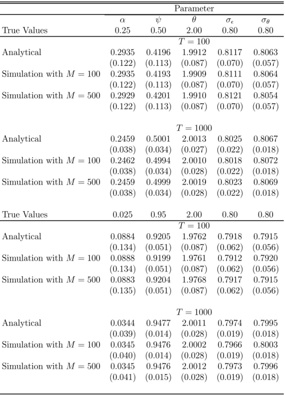
The second set of Monte-Carlo experiments estimates the model parameters using the method of Maximum Likelihood. Since the likelihood function is not always continuous on the parameters when the frequency simulator is used, I used the kernel-smoothed frequency simulator with κ = 0.05. The experiment involve sample sizes with T = 100 and T = 1000 observations, and simulated conditional expectations computed with M = 100 and M = 500 paths. In all cases, 100 extra observations were generated in every replication. Then, for the estimation of the model, the initial 100 observations were discarded in order to limit the effect of the starting values used to generate the observations of rt. All results are
based on 200 replications. In each replication, the model was estimated three times. First using the analytical (exact) conditional expectation and then using the simulated conditional expectation with M = 100 and M = 500. Monte-Carlo results are reported in Table 1. In both the small- and large-sample experiments, parameter estimates are close to their true value and to the estimates based on the analytical forecast. As expected, the standard errors are smaller for the sample T = 1000 than for T = 100. Using M = 500 or M = 100 simulated paths yields essentially the same results in the experiments considered, but the former takes roughly three times longer to converge.
6
Interest Rates in Japan
6.1
The Data
The empirical analysis of the model is based on 360 weekly (Tuesday) observations of the one-, three-, six-, and twelve-month nominal interest rates on zero-coupon Treasury bills for Japan. The data source is Datastream. The Datastream mnemonics for the series are JAP1MBL, JAP3MBL, JAP6MBL, and JAP1YBL, respectively. The sample starts on 9 June 1994 and ends on 24 April 2001. Prior to 9 June 1994, there are no observations of the return on the six- and twelve-month Treasury bills in the database. The sample ends on 24 April 2001 because this was the latest available observation at the time data was collected. The rates are quoted at an annual rate and in units of 100 basis points. Empirical results below are also reported in units of 100 basis points.
his-tograms are plotted in Figures 5(A) to 5(D). For most of the sample period, Japanese interest rates have been remarkably close to the zero lower bound. The data features ob-servations as low as 0.03 for the one-month interest rate on 20 May 1999 and 0.06 for the twelve-month interest rate on 29 October 1998. The medians for the one-, three-, six-, and twelve-month interest rates are only 0.44, 0.47, 0.47, and 0.53, respectively. Their distributions are asymmetric, positively skewed, and truncated on the left at the zero lower bound.
The casual observation of the series in Figure 4 suggests a structural change in mid-1995. Contemporaneous accounts indicate that an even more expansionist monetary policy was undertaken by the Bank of Japan starting in the third quarter of 1995 [see The Economist, 16 September 1995 (p. 86)]. This intuition is confirmed statistically by a supF test for structural breaks [Andrews (1993)]. The null hypothesis of zero breaks is rejected in all cases at the 5% level against the alternative of one break.5 The sequential procedure proposed by
Bai and Perron (1998) indicates a break on 29 June 1995 for the one-month interest rate and on 15 June 1995 for the three-, six-, and twelve-month interest rates. Consequently, in the analysis that follows, I consider both the complete sample described above and a subsample from 6 July 1995 to 24 April 2001.
6.2
The Short-Term Interest Rate
The model is calibrated using the one-month interest rate as the short-term interest rate, rt.
The process of r∗
t is described in terms of past realizations of the short-term interest rate
with lag length determined using sequential Likelihood Ratio (LR) tests.6 The conditional
variance of ²t is modeled using a GARCH(1,1) specification [Bollerslev (1986)]: ²t =
√ htvt,
where vt is i.i.d.N (0, 1) and ht= ζ + δ²2t−1+ %ht−1. An advantage of this parameterization
is that it can capture the persistence of the conditional variance in a more parsimonious manner than higher-order ARCH processes. The estimated process are:
rt= ½ r∗ t, if r∗t > 0, 0, otherwise, with
5The supF statistics are 18.01, 18.06, 22.70, and 17.95 for the one-, three-, six-, and twelve-month interest
rates, respectively. The critical value at the 5% level is 8.58. The test was implemented using a code provided to me by Jushan Bai.
6In principle, the model can accommodate a multivariate representation of r∗
t. However, many series, like
money and output growth, are unavailable on a weekly basis. Using an univariate process for the short-term interest rate makes the model more parsimonious and allows me to concentrate on a well-defined statistical object, namely the bivariate process (rt, Rt), for the purpose of econometric inference.
r∗ t = −0.0036 + 0.633rt−1 + 0.196rt−2 + 0.186rt−3 + ²t, (0.0059) (0.072) (0.086) (0.058) and ht = 0.005 + 0.671²2t−1 + 0.141h2t−1, (0.0008) (0.128) (0.075)
for the sample 9 June 1994 to 24 April 2001; and r∗ t = 0.0185 + 0.598rt−1 + 0.127rt−2 + 0.214rt−3 + ²t, (0.0106) (0.079) (0.077) (0.055) and ht = 0.004 + 0.539²2t−1 + 0.223h2t−1, (0.0008) (0.111) (0.079)
for the sample from 6 July 1995 to 24 April 2001.
A standard misspecification test for ARCH-type models is the Ljung-Box Q-statistic applied to the standardized residuals squared. If the ARCH model is correctly specified, then the residuals corrected for heteroskedasticity and squared should be serially uncorrelated. Under the null hypothesis of no autocorrelation, the Q-statistic is distributed chi-square with degrees of freedom equal to the number of autocorrelations. Table 2 reports the Q-statistic for up to ten autocorrelations. Since all statistics are below the 5% critical value of the appropriate distribution, the null hypothesis cannot be rejected at the 5% level. Hence, it would appear that a GARCH(1,1) model captures adequately the conditional heteroskedasticity in the Japanese one-month interest rate.
6.3
Implied Long-Term Interest Rates
I examine now the implications of the nonnegativity constraint for the term-structure using the estimated process for the short-term interest rate in Japan.7 The conditional expecta-tions of rt are computed using the frequency simulator proposed in Section 4. The
condi-tional variance of ²twas set to its unconditional mean σ²2 = 0.004/(1−0.539−0.223) = 0.0168.
Figure 6(A) plots the conditional expectations of the Japanese one-month interest rate for different values of the current one-month rate and for different horizons (s). Notice that as a result of the zero lower bound, the conditional expectations “bend” upward at low nominal
7These results are based on estimates from the period 6 July 1995 to 24 April 2001. Using estimates
from the period 9 June 1994 to 24 April 2001 yielded essentially the same results and are available from the author upon request.
interest rates. Thus, the conditional expectations are a nonlinear and convex function of the current short-term interest rate. This effect is reminiscent of the honeymoon effect in exchange-rate target-zone models in continuous [see Krugman (1991)] and discrete time [see Pesaran and Samiei (1995)]. At low nominal interest rates, the range of possible future realizations of rt is larger above than below the current rate as a result of the nonnegativity
constraint. Consequently, the conditional forecast of future short-term rates is well above the current rate. This effect increases as rt approaches the zero lower bound and is more
pronounced as the horizon increases.
It is interesting to compare these conditional expectations with the ones obtained using a linear forecasting model that ignores the effect of the zero lower bound on expectations. The conditional expectations using a linear model are plotted in Figure 7(A). In this case, the forecasts are linear functions of the current one-month interest rate. For interest rates well above the nonnegativity constraint, the forecasts obtained using the linear and nonlinear models are identical. For interest rates close to the zero lower bound, the forecasts using the nonlinear model are above the ones of the linear model at all horizons. As we will see below, this translates into significantly different predictions for the long-term interest rates. The two-, three-, six-, and twelve-month interest rates predicted by the nonlinear model are plotted in Figure 6(B). Because long-term interest rates depend on the average forecast of future short-term rates, they are nonlinear and convex functions of the current short-term interest rate. As a result of the nonnegativity constraint, long-term interest rates “bend” upward at low short-term interest rates.
The two-, three-, six-, and twelve-month interest rates predicted by the linear model are plotted in Figure 7(B). Since the conditional expectations of the short-term interest rate are linear functions of rt, long-term interest rates are also linear on rt. For one-month
interest rates well above the nonnegativity constraint, the long-term interest rates predicted by the linear and nonlinear models are the same. For one-month interest rates close to the nonnegativity constraint, the nonlinear model predicts substantially higher long-term interest rates than the linear model. In other words, the nonlinear model predicts a steeper term-structure than the linear model at low short-term interest rates. Saunders (2000, p. 1064) reports that the average difference between the nominal rates on long-term government bonds and one-month Treasury bills in Japan passed from 35 basis points in 1984 (when the average one-month rate was 6.34) to 235 in 1998 (when the average one-month rate was 0.22).
In the linear forecasting model certainty-equivalence holds and the conditional expec-tations of the one-month rate do not depend on its volatility. On the other hand, in the nonlinear model, the conditional variance of ²tcan affect the conditional forecast of rt. Recall
that for a two-period bond, analytical results in Section 2 indicate that, given the short-term rate, E(rt+1|It) and Rt are increasing on σ². Figures 8(A) and 8(B) examine the effect of
the conditional standard deviation of the Japanese one-month rate on the conditional ex-pectations of rt for different horizons, and on the long-term interest rate. For these graphs,
the current one-month interest rate is fixed to its sample average. The current conditional standard deviation of the one-month rate varies between 0.04 and 0.86. This range corre-sponds to the one taken by the conditional standard deviation of the Japanese one-month interest rate in the sample period. Future conditional standard deviations are forecasted using the GARCH(1,1) process estimated above. Notice in Figure 8(A) that the conditional expectations of the one-month interest rate are increasing functions of the current condi-tional standard deviation. As anticipated by the analytical results in Section 2, the relation is nonlinear and convex. As a result, long-term interest rates are also increasing, nonlinear, and convex on the current conditional standard deviation of the one-month rate. For low values of the conditional standard deviation, the effect is small regardless of the maturity. As the conditional standard deviation rises, the effect becomes larger specially for longer term maturities. Black (1995, p. 1373) argues that option pricing considerations imply that the long-term interest rate should rise with the volatility of the short-term rate. However, for the data set considered, 90% of the observations of the conditional standard deviation are below 0.2 and only 2% are above 0.4. Thus, Figure 8(B) suggests that the volatility effect described by Black is likely of play a minor role in the determination of the Japanese long-term interest rates.
6.4
Comparison with Linear Forecasting Model
One strategy to compare empirically the relative merits of the linear and nonlinear forecasting models, is to compute forecasts error statistics. To that effect, I compute the Sum of Squared Errors (SSE): SSE = T X t=1 (Rt− ˆRt)2,
and the Sum of Absolute Errors (SAE): SAE =
T
X
t=1
|Rt− ˆRt|,
where Rtis the observed Japanese long-term interest rate and ˆRtis the rate predicted by the
model. These statistics are reported in Table 3. The linear model constructs the long-term interest rate using linear forecasts the one-month interest rate. The nonlinear models take
into account the effect of the zero lower bound on expectations, but differ on their treatment of the conditional standard deviation of ²t. The nonlinear model I computes the forecasts of
the one-month interest rates using the GARCH(1,1) estimates of the conditional standard deviation of ²t. The nonlinear model II fixes the conditional standard deviation of ²t to its
unconditional mean.
With only one exception, the nonlinear models deliver smaller forecast errors than the linear forecasting model. The gain of using the nonlinear models is numerically small but might be economically important when pricing bonds and other debt instruments. Note that the difference in forecasts errors appear to be more important for longer than shorter maturities In all cases, the nonlinear model that assumes a constant conditional standard deviation for the one-month rate delivers smaller SSE and SAE than the nonlinear model that allows volatility to affect the conditional expectation of rt. Recall that for one-month
interest rates well above the zero lower bound, the linear and nonlinear models predict the same long-term interest rate. The reason the nonlinear model delivers smaller forecasts errors in the sample is because at very low one-month interest rates, the linear model under-predicts the long-term rate while the nonlinear model under-predicts the steeper term structure observed in the data. This can be seen in Figure 9 that plots the yield curve for two different values of the current short-term interest rate. For the very low value of 0.05, the nonlinear model predicts a steeper yield curve than the linear model. The steeper yield curve appears to fit better the observed returns in the Japanese data set. For the larger (though still low) value of 0.3, the difference between both models is smaller, as expected, and the forecasts errors are roughly of the same magnitude.
6.5
Impulse-Response Analysis
I now examine the response of the long-term interest rate associated with a change in the short-term interest rate. In the case of linear models of the term structure, an innovation to the short-term rate yields movements in the long-term rate that are symmetric, proportional, and history-independent. More generally, for linear models, the impulse-response associated with a shock of size 1 (standard deviation) would be the mirror image of the response to a shock of size −1, one-half the response of shock size 2, and independent of the moment the shock is assumed to take place. In contrast, for nonlinear models of the term structure, the response of the long-term rate varies with the size and sign of the shock and the initial value of the short-term rate.8
8For the impulse-response analysis of nonlinear systems see Gallant, Rossi, and Tauchen (1993), and
Figures 10 to 14 plot (respectively) the response of the three-month, six-month, twelve-month, two-year and five-year interest rates to an increase and to a decrease 0.25 percentage points (25 basis points) in the short-term rate under the linear and nonlinear models. In constructing these responses, the conditional variance and one-month interest rate are fixed to their unconditional means. Note first that the response of the long-term rate under the linear model is symmetric. The response to an increase of 0.25 percentage points in the one-month rate is the mirror image of the response to a decrease of 0.25 percentage points. For the nonlinear model that takes into account the effect of the zero lower bound on expectations, the response of the long-term rate is asymmetric. The increase in the long-term rate when the one-month rate increases by 0.25 percentage points is larger (in absolute value) than the decrease in the long-term rate when the one-month rate decreases by 0.25 percentage points. For shorter maturities, like the three- and six-month interest rates, this asymmetric effect is negligible. For longer maturities, this asymmetric effect is larger. For example, when the one-month interest rate increases (decreases) by 0.25 percentage points, the twelve-month rate increases (decreases) by 0.113 (0.099) percentage points, the two-year rate increases (decreases) by 0.086 (0.072) percentage points, and the five-year rate increases (decreases) by 0.045 (0.037) percentage points. This asymmetric effect is proportionally larger for longer maturities.
The linear model predicts that a decrease in the one-month interest rate by 0.25 percent-age points decreases the twelve-month, two-year, and five-year interest rates by 0.120, 0.098, and 0.058 percentage points, respectively. The nonlinear model predicts a decrease by 0.099, 0.072, and 0.037 percentage points, respectively. In both the linear and nonlinear models, the effect on the long-term interest rate decreases with the horizon but it is more severe for the nonlinear model. In order to understand the difference in the prediction of both models, it is useful to return to Figures 6(B) and 7(B). Note that under the nonlinear model [Figure 6(B)], the relation between the short- and long-term interest rates is “flatter” than under the linear model [(Figure 7(B)]. This means that under the nonlinear model, that takes into account the effect of the zero lower bound on expectations, changes in the short-term rate induce smaller changes in the long-term rate than under the linear model. Hence, it appears that up to the extent that monetary policy acts by affecting long-term rates through the term structure, its power is considerably reduced at low interest rates.
7
Summary and Discussion
This paper derives the implications of the zero lower bound on interest rates for the term structure under the PEH hypothesis. The empirical predictions of the model that takes
into account the nonnegativity constraint differ sharply from the ones of a benchmark linear model. As a result of the zero lower bound, the long-term interest rate is an increasing, nonlinear, and convex function of the level and conditional standard deviation of the short-term interest rate. The effect of changes in the short-short-term rate on the long-short-term rate are asymmetric and smaller than predicted by a linear model. An increase in the short-term rate leads to an increase in the long-term rate that is larger in magnitude than the decrease in the long-term rate associated with a decrease in the short-term rate of the same size. Forecasts error statistics indicate that the nonlinear model provides a better fit of the Japanese data than a linear model that ignores the effect of the zero lower bound on expectations. The reason the nonlinear model delivers smaller forecasts errors is because at very low interest rates, the linear model under-predicts the long-term rate while the nonlinear model predicts better the steeper term structure observed in the data.
Results using weekly Japanese data suggest that the volatility effect described by Black (1995) is unlikely to play a major role in the determination of long-term interest rates in Japan. The nonlinear and asymmetric effects appear to be more important but it is clear that their magnitude is small, even for the extreme case of Japan. Hence, it is unlikely that the zero lower bound on interest rates have an effect on the term structure in other OECD countries where nominal rates are at historically low levels, but still within safe distance from the nonnegativity constraint. However, additional research is necessary before more conclusive statements can be made.
A
Proof of Proposition 2
Define the standardized normal variable ξt= ²t/σ² and use the definition of ct+1 to write the
process of the short-term rate at time t + 1 as rt+1=
½ E(r∗
t+1|It) + ²t+1, if ξt+1> ct+1,
0, otherwise.
Note that ct+1is known at time t. The conditional expectation of rt+1is the weighted average
E(rt+1|It) = E(rt+1|It, ξt+1> ct+1) Pr(ξt+1 > ct+1)
+E(rt+1|It, ξt+1 ≤ ct+1) Pr(ξt+1≤ ct+1).
Since the forecast E(r∗
t+1|It) = α + ψrt is also known at time t,
E(rt+1|It, ξt+1 > ct+1) = α + ψrt+ E(²t+1|It, ξt+1> ct+1).
Note that
E(rt+1|It, ξt+1≤ ct+1) = 0,
and write [see Maddala (1983, p. 366)]
E(²t+1|It, ξt+1> ct+1) = σ²φ(ct+1)/[1− Φ(ct+1)],
where 1− Φ(ct+1) stands for Pr(ξt+1> ct+1). With these intermediate results
E(rt+1|It) = (α + ψrt)[1− Φ(ct+1)] + σ²φ(ct+1),
B
Proof of Proposition 4
Use the definitions of us,t+s and ct+s to write the process of the short-term rate at time t + s
as
rt+s=
½
E(rt+s∗ |It) + us,t+s, if us,t+s> ct+s,
0, otherwise.
Then, the conditional expectation of rt+s is the weighted average
E(rt+s|It) = E(rt+s|It, us,t+s> ct+s) Pr(us,t+s> ct+s),
+E(rt+s|It, us,t+s ≤ ct+s) Pr(us,t+s≤ ct+s). (23)
Since the forecast E(r∗
t+s|It) is known at time t,
E(rt+s|It, us,t+s > ct+s) = E(rt+s∗ |It) + E(us,t+s|It, us,t+s > ct+s).
Also
E(rt+s|It, us,t+s ≤ ct+s) = 0.
Plugging these intermediate results into (23), and using Pr(us,t+s > ct+s) = 1− Fs(ct+s), the
conditional expectation of the short-term rate at time t + s is E(rt+s|It) = £ E(rt+s∗ |It) + E(us,t+s|It, us,t+s > ct+s) ¤ [1− Fs(ct+s)] , as claimed.
Table 1. Monte Carlo Results Parameter α ψ θ σ² σθ True Values 0.25 0.50 2.00 0.80 0.80 T = 100 Analytical 0.2935 0.4196 1.9912 0.8117 0.8063 (0.122) (0.113) (0.087) (0.070) (0.057) Simulation with M = 100 0.2935 0.4193 1.9909 0.8111 0.8064 (0.122) (0.113) (0.087) (0.070) (0.057) Simulation with M = 500 0.2929 0.4201 1.9910 0.8121 0.8054 (0.122) (0.113) (0.087) (0.070) (0.057) T = 1000 Analytical 0.2459 0.5001 2.0013 0.8025 0.8067 (0.038) (0.034) (0.027) (0.022) (0.018) Simulation with M = 100 0.2462 0.4994 2.0010 0.8018 0.8072 (0.038) (0.034) (0.028) (0.022) (0.018) Simulation with M = 500 0.2459 0.4999 2.0019 0.8023 0.8069 (0.038) (0.034) (0.028) (0.022) (0.018) True Values 0.025 0.95 2.00 0.80 0.80 T = 100 Analytical 0.0884 0.9205 1.9762 0.7918 0.7915 (0.134) (0.051) (0.087) (0.062) (0.056) Simulation with M = 100 0.0888 0.9199 1.9761 0.7912 0.7920 (0.134) (0.051) (0.087) (0.062) (0.056) Simulation with M = 500 0.0883 0.9204 1.9768 0.7917 0.7915 (0.135) (0.051) (0.087) (0.062) (0.056) T = 1000 Analytical 0.0344 0.9477 2.0011 0.7974 0.7995 (0.039) (0.014) (0.028) (0.019) (0.018) Simulation with M = 100 0.0345 0.9476 2.0002 0.7966 0.8003 (0.040) (0.014) (0.028) (0.019) (0.018) Simulation with M = 500 0.0345 0.9476 2.0012 0.7973 0.7996 (0.041) (0.015) (0.028) (0.019) (0.018)
Notes: T is the sample size. M is the number of paths generated to compute the conditional expectation. The experiments were based on 200 replications.
Table 2. Q-statistic for Autocorrelation
Standardized Squared Residuals of the One-month Interest Rate Q-statistic
Sample 9 June 1994 to 6 July 1995 to Autocorrelation 24 April 2001 24 April 2001
1 0.111 0.004 2 0.157 0.623 3 0.167 0.629 4 0.614 0.718 5 3.930 0.743 6 3.970 0.812 7 5.330 1.852 8 5.336 1.878 9 6.482 2.134 10 7.541 2.384
Notes: Under the null hypothesis of no autocorrelation, the Q-statistic is distributed chi-square with degrees of freedom equal to the number of autocorrelations.
Table 3. Comparison of Linear and Nonlinear Models
Measure Maturity Model
(in months) Linear Nonlinear I Nonlinear II A. 9 June 1994 to 24 April 2001 SSE 3 6.23 6.15 6.04 6 8.47 8.29 7.98 12 20.09 18.84 18.30 SAE 3 30.48 30.28 30.07 6 40.09 38.55 38.00 12 64.99 60.87 60.09 B. 6 July 1995 to 24 April 2001 SSE 3 5.97 5.07 5.00 6 6.62 6.61 6.45 12 16.87 16.43 16.30 SAE 3 24.90 25.03 24.84 6 31.39 30.84 30.59 12 50.86 49.68 49.41
Notes: SSE is Sum of Squared Error. SAE is Sum of Absolute Errors. The linear model forecasts the one-month interest rate linearly. The nonlinear model I takes into account the effect of the zero lower bound and the conditional standard deviation of ²t. The nonlinear
model II takes into account the effect of the zero lower bound but fixes the conditional standard deviation of ²t to its unconditional mean.
References
[1] Andrews, D. (1993), “Tests for Parameter Instability and Structural Change with Un-known Change Point,” Econometrica, 61: 821-856.
[2] Bai, J. and Perron, P. (1998), “Estimating and Testing Linear Models with Multiple Structural Changes,” Econometrica, 66: 47-78.
[3] Baillie, R. T., and Bollerslev, T. (1992), “Prediction in Dynamic Models with Time-Dependent Conditional Variances,” Journal of Econometrics, 52: 91-113.
[4] Black, F. (1995), “Interest Rates as Options,” Journal of Finance, 50: 1371-1376. [5] Baxter, M. (1990), “Estimating Rational Expectations Models with Censored Variables:
Mexico’s Adjustable Peg Regime of 1973-1982,” University of Rochester, Mimeo. [6] Cecchetti, S. G., (1988), “The Case of the Negative Nominal Interest Rates: New
Estimates of the Term Structure of Interest Rates during the Great Depression,” Journal of Political Economy, 96: 1111-1141.
[7] Cox, J. C., Ingersoll, J. E., and Ross, S. A. (1985), “A Theory of the Term Structure of Interest Rates,” Econometrica, 53: 385-407.
[8] Fisher, I. (1896), Appreciation and Interest. August M. Kelley Bookseller, New York. [9] Fuhrer, J. C. and Madigan, B. F. (1997), “Monetary Policy when Interest Rate are
Bounded at Zero,” The Review of Economics and Statistics, 79: 573-585.
[10] Gallant, A. R., Rossi, P.E., and Tauchen, G. (1993), “Nonlinear Dynamic Structures,” Econometrica, 61: 871-908.
[11] Geweke, J., Keane, M., Runkle, D. (1994), “Alternative Computational Approaches to Inference in Multinomial Probit Models,” Federal Reserve Bank of Minneapolis, Staff Report No. 170.
[12] Holt, M. T. and Johnson, S. R. (1989), “Bounded Price Variation and Rational Expecta-tions in an Endogenous Switching Model of the US Corn Market,” Review of Economics and Statistics, 71: 605-613.
[13] Koop, G., Pesaran, M. H., and Potter, S. M. (1996), “Impulse Response Analysis in Nonlinear Multivariate Models,” Journal of Econometrics, 74: 119-147.
[14] Krugman, P. (1991), “Target Zones and Exchange Rate Dynamics,” Quarterly Journal of Economics, 106: 669-682.
[15] Lerman, S. and Manski, C. (1981), “On the Use of Simulated Frequencies to Approxi-mate Choice Probabilities,” in Structural Analysis of Discrete Data with Econometric Applications, edited by C. Manski and D. McFadden. MIT Press, Cambridge.
[16] McCallum, B. T. (2000), “Theoretical Analysis Regarding a Zero Lower Bound on Nominal Interest Rates,” Journal of Money, Credit and Banking, 32: 870-904.
[17] McFadden, D. (1989), “A Method of Simulated Moments for Estimation of Discrete Response Models without Numerical Integration,” Econometrica, 57: 995-1026.
[18] Maddala, G. S. (1983), Limited-Dependent and Qualitative Variables in Econometrics, Econometric Society Monograph No. 3. Cambridge University Press, Cambridge. [19] Newey, W. and West, K. (1987), “A Simple Positive Semi-Definite, Heteroskedasticity
and Autocorrelation Consistent Covariance Matrix,” Econometrica, 55: 703-708. [20] Orphanides, A. and Wieland, V. (1998), “Price Stability and Monetary Policy
Effec-tiveness when Nominal Interest Rates are Bounded at Zero,” Board of Governors of the Federal Reserve System, Mimeo.
[21] Pesaran, M. H. and Ruge-Murcia, F. J. (1999), “Analysis of Exchange Rate Target Zones Using a Limited-Dependent Rational Expectations Model with Jumps,” Journal of Business and Economic Statistics, 17: 50-66.
[22] Pesaran, M. H. and Samiei, H. (1992), “Estimating Limited-Dependent Rational Ex-pectations Models: With an Application to Exchange Rate Determination in a Target Zone,” Journal of Econometrics, 53: 141-163.
[23] Pesaran, M. H. and Samiei, H. (1995), “Limited-Dependent Rational Expectations Mod-els with Future Expectations,” Journal of Economic Dynamics and Control, 19: 1325-1353.
[24] Ripley, B. D. (1987), Stochastic Simulation, John Wiley & Sons: New York.
[25] Ruge-Murcia, F. J. (2000), “Uncovering Financial Markets’ Beliefs about Inflation Tar-gets,” Journal of Applied Econometrics, 15: 483-512.
[26] Saunders, A. (2000), “Low Inflation: The Behavior of Financial Markets and Institu-tions,” Journal of Money, Credit and Banking, 32: 1058-1087.