Maalaoui Chun : KAIST, Graduate School of Finance, 87 Hoegiro, Dongdamoongu, Seoul, South Korea, 130-722;
phone : +822 958-3424
olfa.maalaoui@gmail.com
Dionne : HEC Montréal, 3000 Chemin de la Côte-Sainte-Catherine, Montréal, Québec, Canada H3T 2A7; phone :
+514 340-6596
georges.dionnne@hec.ca
François : HEC Montréal, 3000 Chemin de la Côte-Sainte-Catherine, Montréal, Québec, Canada H3T 2A7; phone :
+514 340-7743
pascal.francois@hec.ca
We are indebted to Albert Lee Chun for extensive discussions, comments and suggestions. We thank an anonymous referee, Hank Bessembinder (the editor), Jin Seo Cho, Jens Dick-Nielsen, Jan Ericsson, Kwangoo Kang, David Lando, Sergei Rodionov, Ilya Strebulaev, Simon van Norden and Andrea Vedolin; and seminar participants at the 2010 Econometric Society World Congress, 2010 World Congress of the Bachelier Finance Society, 2009 C.R.E.D.I.T. Conference, 20th (EC)2 Conference on Real Time Econometrics, 4th International Conference on Asia-Pacific Financial Markets; as well as the University of Southern California, KAIST Graduate School of Finance, Korea University, and Sungkyunkwan University for helpful comments. We acknowledge financial support from the Institut de Finance Mathématique de Montréal (IFM2), the Tunisian Ministry of Education, the Canada Research Chair in Risk Management, the Center for Research on e-finance and KAIST Graduate School of Finance.
Cahier de recherche/Working Paper 09-29
Detecting Regime Shifts in Credit Spreads
Olfa Maalaoui Chun Georges Dionne Pascal François
Première version/First Version : Août/August 2009
Version révisée/Revised : Mars/March 2013
Abstract:
Using an innovative random regime shift detection methodology, we identify and confirm two distinct regime types in the dynamics of credit spreads: a level regime and a volatility regime. The level regime is long lived and shown to be linked to Federal Reserve policy and credit market conditions, whereas the volatility regime is short lived and, apart from recessionary periods, detected during major financial crises. Our methodology provides an independent way of supporting structural equilibrium models and points toward monetary and credit supply effects to account for the persistence of credit spreads and their predictive power over the business cycle.
Keywords: Credit spread regimes, level regimes, volatility regimes, credit cycle,
economic cycle, monetary effect, credit supply effect
I. Introduction
It is widely known that most existing credit risk models fail to generate the high levels of credit spreads that match empirical observations. For instance, Huang and Huang (2012) find that standard structural models, when calibrated to match his-torical default and recovery rates, all generate counterfactually low levels of credit spreads. The gap between observed and model-implied credit spreads is known in the literature as the credit spread puzzle.1 While most existing studies addressing
the credit spread puzzle focus on the level of credit spreads, Chen, Collin-Dufresne, and Goldstein (2009) find that standard structural models also fail to match the high volatility of credit spreads. This phenomenon, which is distinct from the credit spread level puzzle, is referred to as the credit spread volatility puzzle. By accounting for the countercyclical nature of default, the authors show that the habit formation model (Campbell and Cochrane (1999)) successfully captures the level and volatility of the BBB–AAA spread. However, this model is unable to explain either the level or the volatility of the corporate–Treasury spread, thus leaving questions about the behav-ior of corporate credit spreads over the risk-free rate unanswered.
The literature has often espoused the theory of countercyclical behavior in credit spread dynamics (Fama and French (1989), Stock and Watson (1989), Chen (1991)).
1The credit spread puzzle refers to the spread between corporate bond yields and treasuries. Stan-dard structural models that only account for the effect of default fail to completely capture the BBB– Treasury spread. One reason is that the spread can be driven by nondefault factors such as tax dif-ferentials, liquidity, and macroeconomic factors (e.g., Collin-Dufresne, Goldstein, and Martin (2001), Elton, Gruber, Agrawal, and Mann (2001)).
However, more recent empirical studies only provide weak evidence supporting the link between economic cycles and the cyclical patterns in credit spreads (e.g., Koop-man and Lucas (2005), KoopKoop-man, Kraeussl, Lucas, and Monteiro (2009)). A possible reason for this weak evidence is that the nature of the relation between credit spreads and macroeconomic factors may vary across economic regimes. A few studies have in-vestigated the joint variation of macro factors and credit spreads by incorporating the possibility of regime shifts. For instance, David (2008) uses regime models to ad-dress the puzzling occurrence of high credit spreads for firms with low default. Hack-barth, Miao, and Morellec (2006), Bhamra, Kuehn, and Strebulaev (2010), and Chen (2010) significantly extend this literature by showing how macroeconomic factors af-fect firms’ financing policies and yield more realistic credit spreads. However, these contributions imply that both the level and volatility of credit spreads are affected by the same macroeconomic factors.
In this article, we focus on the distinct patterns in the time series of the level and volatility of credit spreads. We shed light on the puzzling disconnect between credit spread cycles and the macroeconomy by identifying and explaining the presence of a disjoint set of level and volatility regimes in the data. To accomplish this, we in-troduce a novel regime detection procedure that has heretofore not been applied in a finance or economics context.2 Our approach builds on the probabilistic-based regime 2Although this methodology was originally motivated by problems in detecting shifts within ecosys-tems, we show how it can be readily adapted for use with time series data on corporate bond transac-tions.
shift detection technique of Rodionov (2004), (2005), (2006). The technique has sev-eral advantages over more standard approaches: i) It detects potential breakpoints in the data in real time, ii) it is nonparametric and lets the data speak without imposing a set of priors on the number or timing of the regime shifts, and iii) the incipience of a new level or volatility regime is determined independently of one another’s. In fact, a key contribution of our research is in decoupling the volatility regime from the level regime, which allows us a previously unexplored view into how the level and volatil-ity of credit spreads interact with the macroeconomy. The new method also permits one to verify that the level and volatility of credit spreads can be driven by distinct economic factors.
Our approach adds to the literature on random regime shift detection. As Lu and Perron (2010) assert, one advantage of random regime shift models is their ability to account for abrupt changes in a time series. These models are also flexible as they do not make any restrictions on the number and the magnitude of the shifts. This feature is particularly valuable for modeling credit spread dynamics, which are subject to shocks on top of the business cycle. To the best of our knowledge, our paper is the first to apply a random regime shift model to the study of corporate credit spread dynamics.
We apply our methodology to the time series of credit spreads over the 1987– 2009 period, encompassing three economic cycles, using corporate bond data from the Warga, NAIC, and TRACE databases. Our results are robust across the three dif-ferent datasets. As an additional check, we construct an aggregate index of corporate bond spreads covering the same three recessionary periods using quoted prices from
Bloomberg and Warga datasets. Repeating our tests using this aggregate index yields similar patterns in the data.
We find that credit spreads have multiple regimes in their level and volatility, as opposed to two or a small number of regimes. The high levels of credit spreads always encompass yet often outlast NBER economic recessions. This result is con-sistent with the empirical evidence of Giesecke, Longstaff, Schaefer, and Strebulaev (2011), who find that the average duration of an NBER recession during 150 years of historical data is about half the average duration of a default cycle (1.5 versus 3.2 years). Another result is that shifts in credit spreads actually occur before the economic cycle (especially for low ratings); that is, credit spreads may have some pre-dictive power over a forthcoming recession.3 We also find that volatility is subject
to shorter regimes, which, apart from recessionary periods, tend to coincide with pe-riods of financial distress, such as the Asian financial crisis of 1997, the collapse of Long-Term Capital Management in 1998, and the 2007–2008 financial crisis. This suggests that level and volatility regimes might be linked to differing sets of observ-able economic phenomena. Motivated by these findings, we investigate possible sets of economic forces that may explain these patterns.
Since our empirical methodology does not rely on a particular economic model, an-other important contribution of our paper is to provide an independent assessment of different models in the literature. Chen (2010), and Bhamra, Kuehn, and Strebulaev (2010) examine the impact of macroeconomic cycles on corporate financing decisions
3Gilchrist and Zakrajšek (2012) also document the predictive power of credit spreads on macroeco-nomic fluctuations.
and credit spreads. Chen (2010) proposes a dynamic capital structure model that en-dogenizes firm’s financing and default decisions over the business cycles. In his model, default arises endogenously through firms’ responses to macroeconomic cycles. Con-sistent with our empirical results, the simulated results in his study indicate that de-fault probabilities are countercyclical. The results also generate a few periods of high default rates outside recessions that can be reconciled with our volatility regimes, also detected outside recession periods. However, simulated results do not show the strong persistence that we detect after economic recessions. In Bhamra, Kuehn, and Strebulaev’s (2010) model, risk-averse agents also choose their dynamic capital struc-ture and default times. Credit spreads vary with macroeconomic conditions and re-veal hysteresis. They depend on both the current macroeconomic environment and the state of the economy when the firm refinances its debt. Their spreads are coun-tercyclical, spike up outside recessions sometimes, and show strong persistence after the recession periods, consistent with our results.
In addition to dynamic structural models, we study two other approaches that generate persistence in credit spreads. The first relates to monetary policy and em-phasizes the role of inflation and the stickiness of long-term debt to obtain persistence in credit spreads (Bhamra, Fisher, and Kuehn (2011)). The second, referred to as the financial accelerator, considers frictions in the credit supply and points to the role of debt collateral constraints as a factor of persistence after a first shock to produc-tivity (Bernanke and Gertler (1989), Kiyotaki and Moore (1997)). None of these two approaches considers the volatility of credit spreads. Finally, these works, except for the financial accelerator, do not discuss the predictive power of credit spreads toward
economic cycles, which is another important result of this paper.
To see how these monetary and credit supply effects play a role in shaping the dy-namics of credit spread regimes, we employ the same methodology to identify regime shifts in the time series of the Fed funds rate, along with shifts in the time series of the index of tightening loan standards. By overlaying the detected monetary policy and the credit supply regimes on our credit spread level regimes and NBER reces-sions, we provide exploratory evidence that monetary as well as credit supply effects contribute to the dynamics of credit spreads, their predictive power on the economic cycle, and their persistence over it.
Nevertheless, we find that macroeconomic cycles, monetary policy, and adverse credit market conditions only partially overlap with credit spread volatility regimes. The volatility of credit spreads increases when market uncertainty increases, both during and outside recessions. We test how market uncertainty links our volatil-ity regimes to macroeconomic conditions and find a significant relation between our volatility factor and systematic forces driving both bond and equity risk premia.
The rest of this article is organized as follows. Section II describes the regime shift detection technique. Section III describes the data. Section IV presents the empirical results and Section V links our results to dynamic structural models, monetary pol-icy, adverse credit conditions, and NBER recessions. Section VI further investigates monetary and credit supply effects on credit spread cycles. Section VII explores the link between credit spread volatility and bond and equity risk factors. Section VIII checks the robustness of our results against different data and model specifications and Section IX concludes the paper. The online-appendix provides technical
develop-ments.
II. Regime Shift Detection
The regime shift detection procedure builds on the sequential t-test analysis of regime shifts developed by Rodionov (2004) for shifts in the mean. This procedure lets the data speak without imposing a set of priors on the number or timing of the regime shifts. The approach views credit spread regimes as random in the sense that, at each time t, one cannot predict the existence or the timing of any future breakpoint. The procedure also incorporates extensions of Rodionov (2005), (2006) in that it detects shifts in variance, overcomes problems related to the way test statistics deteriorate toward the end of time series, and accounts for hidden autocorrelation in the data that may lead to the detection of false regimes.
Alternative methods for detecting break dates in time series can be found in the econometrics literature on structural changes and include Gordon and Pollak (1994), Bai and Perron (1998), (2003), Chib (1998), Chen, Choi, and Zhou (2005), Perron and Qu (2006), Pesaran, Pettenuzzo, and Timmermann (2006), Davis, Lee, and Rodriguez-Yam (2008), Giordani and Kohn (2008), Maheu and McCurdy (2009), and Bai (2010). Our method differs from these works by offering a technique that detects breaks in the mean and the volatility of credit spreads independently of one another. The advan-tage is that economic shocks affecting the volatility of credit spreads will not unduly influence the detection of shifts in the levels and vice versa. Thus, our method allows level and volatility regimes to have their own patterns and to link up differently with
economic phenomena. It is also a real-time method in the sense that possible breaks can be detected as new data arrive and, in contrast to parametric techniques, it is free from any assumption about the number and timing of the breaks.4
The regime detection test is performed in two stages. A first test identifies poten-tial regime shifts in the data and a second test either accepts or rejects the potenpoten-tial shifts based on subsequent data. We first detect shifts in the mean of the level of credit spreads. After purging the level regimes from the data, we detect shifts in the variance of the residuals.
A. The Dynamics of Credit Spreads
Consider that data on credit spreads are represented by the following time series fYt; t = 1; :::; ng. Suppose Yt is described by an autoregressive model:
(1) Yt ft = (Yt 1 ft 1) + "t;
where ftcaptures a potentially time-varying mean, is the autocorrelation coefficient,
and "t is a normally distributed independent random variable with zero mean and
variance 2. We want to test if time t = c is a breakpoint for credit spreads shifting
from one regime with mean value 1 to another regime with mean value 2. Formally,
4The regimes identified in the literature on credit spreads are always defined in terms of the pa-rameters of the model of the credit spread, not formally on the volatility of the spreads. The two different regimes estimated produce different residual volatilities and are classified as either high- or low-volatility regimes.
ftis given by (2) ft = 8 > > < > > : 1; t = 1; 2; :::; c 1; 2; t = c; c + 1; :::; n:
The regime shift detection tests the null hypothesis H0 : 1 = 2using a two-sample
t-test. We present the details of the test in Section C. The detection method is real-time in that it applies the test to each arrival time of new data. This sequential detection technique is a data-driven analysis that does not require any a priori hypothesis on the existence and timing of regime shifts. In particular, at each time t, one cannot pre-dict the occurrence of any future breakpoint. Therefore, the method aims at detecting random regime shifts.
The presence of a positive autocorrelation coefficient, 0 < < 1 in Equation (1), can generate patterns that resemble regimes in the data that can lead to false rejec-tions of the null hypothesis. When the underlying data contain a stationary first-order autoregressive process with a positive autocorrelation coefficient, such a process is known as a red noise process. Thus, the removal of red noise, which involves esti-mating the AR(1) coefficient (^), is an important preliminary step that facilitates the accurate detection of regime shifts in the data.
B. The Prewhitening Procedure
A common manifestation of red noise is the presence of persistent swings in the data, whereby the observations drift above and then below their mean. The red noise
process is further documented in Appendix A. These patterns are often mistaken for those generated by regimes. Given that the behavior of credit spreads within regimes is characterized by such a process,5standard regime shift detection techniques could
lead to the false detection of regime shifts. By filtering out apparent shifts induced by red noise, we reduce the number of possible spurious breakpoints in the data. We then confirm that the detected breakpoints reflect true shifts in the data.
The difficulty with the prewhitening procedure is in obtaining an accurate esti-mate of the AR(1) coefficient (b) for short subsamples of size n because the traditional techniques, such as ordinary least square, lead to biased estimates for in the pres-ence of regime shifts. This makes it necessary to use subsampling and, since we have relatively short subsamples, we use the inverse proportionality with four corrections (IP4) technique to estimate the autoregressive coefficient.6 The subsampling
proce-dure requires that the subsample size n be less than or equal to the integer part of (m + 1) =3, where m is the average length of a regime interval (Rodionov (2006)). In our case, m and n are expressed in months. For m 6, the subsample size equals three months. In other words, the size of the subsamples must be chosen so that the majority of them do not contain change points. Using a subsampling procedure, the
5For instance, David (2008) shows strong first-order autoregressive (AR (1)) effects in credit spreads with a first-order autocorrelation coefficient of 0.86.
6Two alternative methods are proposed in the literature: the MPK (Marriott and Pope (1954) and Kendall (1954)) and the IP4 techniques (Orcutt and Winokur (1969); Stine and Shaman (1989)). Both methods perform better than the OLS and are similar to one another for n 10. Estimation details using the MPK and IP4 techniques are provided in Appendix B. Rodionov (2006) shows that, based on Monte Carlo estimations, the IP4 technique substantially outperforms the MPK technique for shorter subsamples.
estimate of is the median among subsample estimates.7
After the AR(1) coefficient is accurately estimated and the red noise is removed, the filtered time series is then processed with the regime shift detection method. This filtered time series is given by
(3) Zt= Yt ^Yt 1:
That is, from Equation (1),
(4) Zt= ft ^ft 1+ "t:
Note that, although the red noise is removed from Yt; the filtered process Zt still has
an AR(1) component in our data.8
C. Shifts in the Mean
Let Z1; Z2; Z3; :::; Zt be the filtered credit spread series, with new data arriving
regu-larly.9 When a new observation arrives, we test whether this new observation repre-7As will be demonstrated, in our empirical application, the initial cut-off length m is equal to six months and the subsample size n is equal to three months. For the initial regime, the sample estimate of equals the mean of the two subsample estimates. As long as the regime length is higher than six months, the sample estimate of is the median among subsample estimates.
8Based on Durbin’s h-test and the Breusch-Godfrey LM -test, we reject the null hypothesis of the absence of an AR(1) process in all our subsamples (results available upon request).
9This step follows after checking that the prewhitened data do not suffer from any statistical issues that may bias our results. We address these issues in Appendix C.
sents a statistically significant deviation from the mean value of the current regime. We define as the difference between the mean values of two subsequent regimes that would be statistically significant at the level mean according to the Student
t-test:
(5) = t2m 2mean
q
2s2m=m;
where m is the initial cut-off length of regimes similar to the cut-off point in low-pass filtering and t2m 2
mean is the value of the two-tailed t-distribution with (2m 2) degrees
of freedom at the given probability level mean. The sample variance s2m is assumed
to be the same for both regimes and equal to the average variance over the m-month intervals in the time series:
The initial current regime contains the initial m observed values and the initial new regime contains the subsequent m observed values. The sample mean of the current regime Zcur is known but the mean value of the new regime Znewis unknown:
At the current time tcur = tm+ 1; the current value Zcur qualifies for a shift to the new
regime if it is outside the critical thresholdiZ#crit; Z"crith,
Z"crit = Zcur+ ;
(6)
Z#crit = Zcur ;
where Z"crit is the critical mean if the shift is upward and Z#crit is the critical mean if the shift is downward. If the current value Zcur is inside the range
i
then it is assumed that the current regime has not changed and the null hypothesis H0 about the existence of a shift in the mean at time tcur is rejected. In this case,
the value Zcur is included in the current regime and the test continues with the next
value at tcur = tm + 2. However, if the current value Zcur is greater than Z "
critor less
than Z#crit, the month tcur is marked as a potential change point and the subsequent
data are used to confirm or reject this hypothesis. The test consists of calculating the regime shift index (RSI) that represents a cumulative sum of normalized anomalies relative to the critical mean Zcrit:
(7) RSI = 1 msm
j
X
i=tcur
Zi Zcrit ; j = tcur; tcur+ 1; :::; tcur+ m 1:
If anomalies Zi Zcrit are of the same sign as that at the time of a regime shift
(i.e., positive if the shift is upward and negative if the shift is downward), it would increase the confidence that the shift did occur. The converse is true if anomalies have opposite signs. Therefore, if at any time during the testing period from tcur to
tcur+ m 1 the RSI turns negative when Zcrit = Z"critor positive when Zcrit= Z#crit, the
null hypothesis for a shift at tcur is rejected. We include the value Zcur in the current
regime and continue the test with the next value at tcur = tm+ 2. Otherwise, time tcur
is declared a change point and is significant at least at the confidence level mean: The
D. Shifts in the Variance
The procedure for detecting regime shifts in the variance is similar to that for the mean, except it is based on the F -test instead of the Student t-test. We now work with the residuals f ig left in the data after the means of the detected regimes are
re-moved. The F -test (two-tailed test) consists of comparing the ratio of the sample vari-ances for two successive regimes s2cur
s2
new with their critical value F 1; 2; var
2 , where
F 1; 2; var2 is the value of the F -distribution with 1 and 2 degrees of freedom and
significance level var: In our application 1 = 2 = m 1: The sample variance s2cur is
the sum of squares of i, where i spans from the previous shift point in the variance (which is the first point of the current regime) to tcur 1: At the current time tcur, the
variance s2
new is unknown. For the new regime to be statistically different from the
current regime, the variance s2
new should be equal to or greater than the critical
vari-ance s2"crit if the current variance is significantly increasing. However, if the current variance is significantly decreasing, the variance s2
new should be equal to or less than
s2#crit, where
s2"crit = s2cur F m 1; m 1; var 2 ; (8)
s2#crit = s2cur=F m 1; m 1; var 2 :
If at any time tcur, the current value of cur satisfies the condition, 2
cur> s2"critwhen
the shift is up or 2
cur < s2#critwhen the shift is down, then tcuris marked as a potential
The verification is based on the residual sum of squares index (RSSI), defined as (9) RSSI = 1 m j X i=tcur 2 i s 2
crit ; j = tcur; tcur+ 1; :::; tcur+ m 1:
If at any time during the testing period from tcur to tcur+ m 1; the index turns
negative when s2
crit = s2"crit or positive when s2crit = s2#crit; the null hypothesis about
the existence of a shift in the variance at time tcur is rejected and the value cur is
included in the current regime. Otherwise, the time tcur is declared a change point at
time tcur+ m 1:
III. Data
Credit spreads are obtained from the following three datasets.
The Lehman Brothers/Warga database: This dataset provides information on monthly prices (quote and matrix prices) of U.S. corporate bonds from January 1987 to Decem-ber 1996. We consider only bonds included in the Lehman Brothers’ bond indexes that have quoted rather than matrix prices.
The NAIC database: The NAIC database provides transaction rather than quoted price data for U.S. corporate bonds. Our sample period from the NAIC database spans January 1994 to December 2004. The database accurately reflects trading activity in the bond market from 1994 onward.
The TRACE database: This database only became available in July 2002. The TRACE database reports high frequency data and contains information about almost
all trades in the secondary over-the-counter market for corporate bonds, accounting for 99% of the total trading volume. Our data from TRACE cover the period from October 2004 to December 2009. We employ the filter proposed by Dick-Nielsen (2009) to clean the data of duplicates and other special features.
The characteristics of the bonds are obtained from the Fixed Investment Securities Database. Our three samples (Warga, NAIC, and TRACE) are restricted to fixed-rate U.S. dollar bonds in the industrial sector with a remaining time to maturity between one year and 15 years. We exclude bonds with embedded options (callable, puttable, or convertible), overallotment options, asset-backed and credit enhancement features, and bonds associated with a pledge security. We filter out observations with missing trade details and ambiguous entries (ambiguous settlement data, negative prices, negative time to maturities, etc.). For NAIC and TRACE, we include all bonds whose average Moody’s credit rating lies between AA and BB. For Warga, we only include bonds with ratings AA, A, and BBB, since this database does not contain a sufficient number of BB-rated bonds needed to extract the Nelson–Siegel–Svensson yield curve. Hull, Predescu, and White (2004) show that Treasury bond yields, which are com-monly used as risk-free rates, are contaminated by liquidity, taxation, and regulation issues. We follow their recommendation to use LIBOR-swap rates as the benchmark for risk-free rates. Swap rates are collected from Datastream and LIBOR rates from the British Bankers’ Association. Because swap rates are available only from April 1987, the sample from Warga starts from this date instead of January 1987. To obtain smoothed yield curves for corporate bonds and LIBOR swaps (hereafter swap curves), we use the Nelson–Siegel–Svensson algorithm. We provide the estimation details in
Appendix D and the summary statistics in Appendix E. Overall, credit spreads are consistent with a bond rating structure. High-grade bonds have lower spread levels and volatilities. However, across the three samples, the Warga dataset reports lower levels and volatilities of credit spreads relative to those of the NAIC and TRACE datasets (on average and across ratings).
IV. Estimation Results
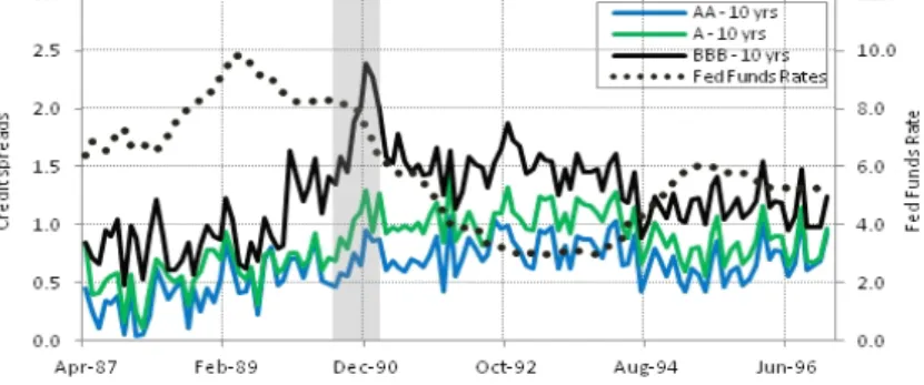
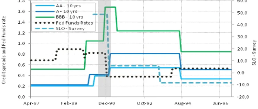
Figures 1 and 2 depict the movements in the time series of credit spreads around the last three NBER recessions, starting in July 1990, March 2001, and December 2007, along with the time series of two macro variables: the Fed funds rate (Figure 1) and the index of tight credit standards (hereafter the Senior Loan Officer (SLO) survey; see Figure 2).10 A common pattern emerges across the three graphs. The
onset of higher levels of credit spreads clearly precedes the start of recessions and lasts until well after the recessions have ended. Although this pattern suggests a connection between the economic cycle and the dynamics of credit spread levels, the fact that high credit spread episodes begin before and persist until after the ends of recessions means that a countercyclical explanation alone is insufficient for linking credit spreads with the macroeconomy. Interestingly, the observed persistence is not unique to credit spread series. As the figures illustrate, both the Fed funds rate and the SLO survey exhibit patterns that are very close to those of credit spreads.
10The SLO Survey is published by the Federal Reserve. It summarizes results of quarterly surveys on bank lending practices, initiated by the Federal Reserve in 1964 and available since April 1990. A detailed description of the survey is given by Lown and Morgan (2006).
Thus, later on we will focus on these two macro variables to understand the economics driving the dynamics of credit spreads.
[Insert Figure 1 and 2 about here]
The plot of the raw data on credit spreads is less revealing when it comes to depict-ing the volatility pattern of credit spreads. Our tests involvdepict-ing a more formal analysis and using our regime detection approach reveal that the level and volatility of credit spreads are, in fact, subject to distinct regimes.
A. The Level Effect
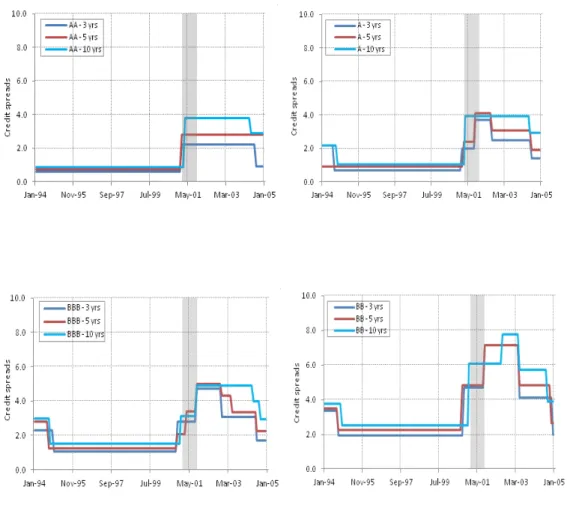
Figure 3 illustrates the results from our level regime detection procedure for 10-year maturity credit spreads. We also list the number of breakpoints, the mean and du-ration of the prior regime, the breakpoint date, the mean and dudu-ration of the new regime and the sign of the detected shift in Appendix F, Table F-1. All reported shifts are statistically significant at the 95% confidence level ( = 5%). These results are obtained with an initial cut-off length m set to its minimum of six months (m = 6) and a Huber parameter of two (h = 2). Other values of m; ; and h are considered in the robustness analysis.
[Insert Figure 3 about here]
Across the three datasets, our procedure detects both positive and negative shifts in the mean. We tend to detect more shifts in the lower rating categories and fewer
shifts in the higher rating categories. In all cases, positive shifts are all detected ei-ther prior to or during NBER recessions. A common pattern across the lower rating categories is the presence of two consecutive positive shifts followed by two consecu-tive negaconsecu-tive shifts. With the exception of the NAIC data (Graph B , Figure 3), the pattern of two consecutive positive shifts is also found across the higher rating cat-egories. This suggests that the transition from a low-level to a high-level regime is likely to occur as a two-step process, especially for lower-rated bonds.
The difference in means between the new and former regimes indicates that the magnitude of the shifts is generally substantial and ranges from 0.15% (AA shift of February 1991) to 3.98% (BB shift of October 2008) as shown in Appendix F, Table F-1.
Figure 3 also depicts where breakpoints are located with respect to the NBER economic cycle. The emerging pattern can be described as follows. First, we detect two consecutive upward shifts around each recession. The first positive shift is located around the official beginning date of the recession and the second one during this same recession. Interestingly, the shifting trend generally starts from the lower-grade bonds and then disseminates across all ratings.11
Second, spreads across all ratings do not instantly revert to their original levels at the end of an NBER recession. Instead, they exhibit persistence. It takes more than three years for credit spread levels to return to their initial levels preceding the 1990–1991 and 2001 recessions. This gradual reversion is completed after one or two downward shifts, depending on the rating category. For the 2007–2009 recession,
the NBER announced on September 20, 2010, that the recession ended in June 2009. Indeed, we detect the first negative shifts in June 2009 for A, BBB, and BB spreads and in July 2009 for AA spreads (Appendix F, Table F-1). As of December 2009 (the latest date in our sample), these spreads are still high and have not yet reverted to their original levels, consistent with the persistence pattern documented earlier. Again, as observed with the upward shifts, we note that the downward shifting trend originates with the lower-grade bonds.
The pattern previously identified with the 10-year credit spreads generally holds for shorter maturities (an illustration is provided in Figure F-1 in Appendix F). How-ever, both first positive and first negative shifts are typically detected earlier for shorter maturities. This aspect is more pronounced for lower ratings. This suggests that spreads with lower ratings and shorter maturities are the first to perceive up-coming downturns.
B. The Volatility Effect
We address the question of whether regimes of credit spread volatilities share the same patterns as regimes of credit spread levels. Our technique is precisely built to answer this question since it allows us to extract true volatility regimes that are independent from level regimes.12
We illustrate our results in Figure 4 and summarize them as follows. First, posi-tive shifts in the volatility are detected around the same time as posiposi-tive shifts in the
12Because volatility has a more straightforward economic meaning than variance, we use the term volatility regime to designate the variance regime.
level. Volatilities across ratings all shift up during recessions. We report details on the statistics pertaining to volatility breakpoints in Table F-2 of Appendix F. We also detect volatility breakpoints without significant changes in the levels. Outside re-cessionary periods, these volatility regimes highlight other adverse financial events. For example, during the period of the Asian financial crisis (officially starting in July 1997), the BBB and BB spreads are in high-volatility regimes. In addition, during the collapse of LTCM (which officially occurred in October 1998), all ratings (AA to BB) are in high-volatility regimes.
[Insert Figure 4 about here]
Our results refute a close link between the level and volatility regimes of credit spreads. We note that in most cases volatility regimes are short and not gradual, contrary to level regimes. Indeed, we detect both a level effect and a volatility effect at the beginning of NBER recessions. However, at the end of recessions, the volatility regimes show no persistence. In addition, as Figure 3 indicates, volatility regimes are not necessarily limited to recessions; rather, they result from significant shocks to the economy, including recessions.
Thus, different sets of economic phenomena drive episodes of high levels and high volatilities of credit spreads. Understanding these economic underpinnings could provide useful insights into decomposing and forecasting changes in credit spreads. Specifically, we have good reason to believe that level regimes are more closely con-nected with real activity, although their persistence and predictive ability remain to be explained. The pattern observed in volatility regimes also calls for specific
investi-gation.
V. Detected Versus Model-Implied Credit Spread Regimes
A. Structural Equilibrium Models
Our regime detection technique is a model-free opportunity to compare the actual cyclical dynamics of credit spreads with those implied by the theoretical literature. This section relates our empirical findings to the characteristics of credit spread dy-namics that arise endogenously in different strands of models.
Structural equilibrium models, initiated by Hackbarth, Miao, and Morellec (2006) and Chen, Collin-Dufresne, and Goldstein (2009), examine the impact of macroeco-nomic cycles on corporate financing decisions and credit spreads. The recent contri-butions of Chen (2010) and Bhamra, Kuehn, and Strebulaev (2010) show that time-varying macroeconomic conditions can help solve the credit spread puzzle. In these two models aggregate consumption and firms’ earnings are exogenous, but their drift and volatility depend on the business cycle determined by a Markov chain. Firms decide on how much debt to hold, when to restructure the debt, and when to default based on their cash flows and macroeconomic conditions.
Chen (2010, fig. 6) reports simulated economic cycles. Recessions correspond to negative expected consumption growth. Unfortunately, the author analyzes default rates but not credit spreads. Default rates are countercyclical in the sense that most of the high default rates (clustering of defaults) arrive in recessions. Thus, credit
spreads should spike when the economy enters a bad state, which is consistent with our detected regimes. However, Chen’s (2010) default rates promptly decrease every time the recession is over. The author’s simulations do not reproduce the persistence in credit spreads that we detect. Finally, we note that the author’s model also gen-erates few periods of high default rates outside recessions. This model output can be reconciled with the credit spread volatility regimes that we detect outside recessions. For Bhamra, Kuehn, and Strebulaev (2010), default rates and credit spreads are also endogenously countercyclical. Figure 3 of their article reports the time series of credit spreads and default rates in the simulated economy. As in Chen (2010), the default rates are countercyclical and some default episodes also occur outside recessions. Most importantly, credit spread levels exhibit persistence after recessions. As explained by the authors, this behavior is driven by shareholders’ optimal default policy. The default boundary that they select depends not only on the current state of the economy, but also on the state prevailing at the previous refinancing time. This creates hysteresis in the distance to default, which is reflected in credit spreads being persistently high after the recession.
In sum, our findings provide some support for the structural equilibrium models. However, three important detected features in our results are not entirely captured by these models. First, the level and volatility of credit spreads exhibit distinct cycles. Chen (2010) and Bhamra, Kuehn, and Strebulaev (2010) do not explicitly examine credit spread volatility regimes. Second, the credit spread level cycle outlasts the economic recession. In Bhamra, Kuehn, and Strebulaev (2010) this effect is generated by introducing path dependence in the distance to default. Third, shifts in credit
spreads actually occur before the economic cycle (especially for low ratings); that is, credit spreads may have some predictive power over the forthcoming recession. None of the previously cited structural equilibrium models captures this predictive aspect, because the credit spread cycle is tightly linked to the economic cycle and essentially the start of a recession triggers a surge in credit spreads.
B. Models with Monetary Effects
The discrepancies between our detected credit spread regimes and those implied by the structural equilibrium models may stem from incomplete modeling of the business cycle. For instance, Bhamra, Kuehn, and Strebulaev (2010) acknowledge that their model generates insufficient comovement between credit spreads and equity returns volatility and points toward the monetary policy as a potential missing factor.
Interestingly, the model of Bhamra, Fisher, and Kuehn (2011), which takes mone-tary effects into account, can also generate persistence in credit spread dynamics. In this structural model, corporate default decisions depend on monetary policy through its impact on expected inflation. Since firms finance with fixed-rate nominal debt, a monetary policy shock (such as a decrease in the Fed funds rate following a tightening of credit standards) lowers expected inflation, which, in turn, makes debt refinancing more difficult and induces firms to maintain high leverage. As a consequence, credit spreads exhibit persistence. The presence of deadweight bankruptcy costs amplifies what Bhamra, Fisher, and Kuehn (2011) call a debt-deflationary spiral.
financ-ing frictions that emerge directly from the nature of long-term debt. Nevertheless, as Bhamra, Fisher, and Kuehn (2011) acknowledge, other non-monetary types of financ-ing frictions, such as shocks to the credit supply, can have a similar impact on credit spread dynamics.
C. Models with Credit Supply Effects
The strand of literature related to the theory of financial accelerators (initiated in particular by Bernanke and Gertler (1989), King, (1994), Kiyotaki and Moore (1997)) considers information asymmetry and the high cost of external financing as frictions in the credit market that, in turn, amplify the effect of shocks on aggregate produc-tivity and extend periods of high credit risk premiums.
Not only does the financial accelerator mechanism generate persistence in credit spreads, but it also entails that credit spread regimes actually precede economic cy-cles, two patterns that are strongly supported by our regime detection technique. Indeed, the financial accelerator literature claims that an increase in credit spreads reflects a tightening of the credit supply and causes economic activity to slow down. Consistent with this view, Gilchrist and Zakrajšek (2012) provide recent evidence that surges in credit spreads actually precede NBER recessions and show that an in-crease in excess bond premium causes a drop in consumption, output, and investment. Mueller (2009) provides another empirical study supporting the predictive power of credit spreads as well as their persistence, induced by the financial accelerator mech-anism.
In their general equilibrium model, Gomes and Schmid (2010) examine shocks on the credit supply in the transmission channel between credit spreads and real activity. In their model, tightening credit conditions lowers the value of outstanding debt and therefore the wealth of households/investors. This, in turn, increases the cost of future debt financing and forces firms to reduce their investment and future output. Although credit supply shocks are not a necessary ingredient in their model (the predictive power of credit spreads is initially driven by endogenous fluctuations in risk aversion), the authors show that the inclusion of these shocks allows for more realistic correlations between macro and financial variables (see Gomes and Schmid (2010), Table 4).
VI. Detecting Regimes in Monetary Policy and Credit
Supply
We now look at additional empirical evidence of the link between credit spreads, mon-etary policy, and the credit supply.
A. Preliminary Tests
We analyze the Fed funds rate time series as a proxy for monetary policy. Regarding the credit supply effect on credit spreads, we use the SLO Survey data as a measure of financial institutions’ willingness to lend.13 More precisely, we use the net percentage 13Some authors (e.g., Lown and Morgan (2006)) have used these data as a measure of subjective perception about the credit market activity (i.e., market sentiment). Other authors (Mueller (2009),
of banks tightening their lending practices, since the Federal Reserve relies on this information in formulating monetary policy actions.14
The Fed funds rate appears as an inverse mirror of the dynamics of credit spreads (Figure 1). Correlation coefficients are generally very high. For instance, the cor-relations between AA spreads and the Fed funds rate are, respectively, -0.50, -0.95, and -0.70 for Graphs A to C. Typically, the Fed anticipates a recessionary period by watching the survey (among other factors) and responds to it by lowering short rates. This economic stimulus continues until credit conditions become loose for firms and banks. The SLO Survey, plotted in Figure 2, shows how periods of high levels of credit spreads correspond to periods of adverse credit conditions (positive values in the SLO Survey data).
Granger causality tests reported in Appendix G show some evidence of feedback effects between credit spreads and the short rate. However, the Fed funds rate seems to lead investment grade spreads in most cases while BB spreads leads the Fed funds rate in all cases, indicating that low-grade spreads are more forward looking than high-grade spreads. In the case of the SLO Survey, we always obtain a unidirectional causal relation from the survey to credit spreads, supporting the idea that credit supply constraints may initiate credit cycles.
Finally, impulse responses reported in Appendix H show that credit spreads
re-Gilchrist and Zakrajšek (2012)) instead use these data as an objective measure of credit conditions (i.e., the tightness of credit standards). In this paper we adhere to the latter interpretation.
14The net percent of tightening equals the number of respondents reporting tightening standards less the number reporting easing divided by the total number reporting.
spond instantaneously to shocks in the survey and to shocks in the Fed funds rate. In both cases, the effect of the shocks persists for several months for all rating classes (Figure H-1). However, a shock to credit spreads has generally smaller and delayed effects on the SLO Survey and the Fed funds rate.
We extend the analysis by applying our regime detection technique on both the Fed funds rate and the SLO Survey time series. Using the same parameters and confidence level, we overlay the detected regimes on top of the credit spread regimes in Figure 3. We list the mean and duration of the prior regime, the number and dates of the breakpoints, the mean and duration of the new regime, and the sign of the detected shift in Table I-1 of Appendix I. The results are analyzed in the next two subsections.
B. SLO Survey Regimes and Credit Spreads Regimes
Level regimes (rather than volatility regimes) are likely to drive the close connection documented in Figures 1 and 2 between credit spreads, monetary policy, and the credit supply. Across the three graphs, SLO Survey data report tightening standards several months ahead of each recession. Specifically, two tightening credit regimes precede each recessionary period, thus driving the two-step regime process observed with credit spread levels. The difference in levels between the two tightening regimes is substantial. For instance, after the 1991 recession (SLO Survey data not available before the recession), we detect a first positive SLO survey regime in October 1998 that lasts till June 2000 (Panel B of Table I-1 of Appendix I). This regime indicates
that, on average, 14.91% of banks tightened their standards. Thereafter, a second positive regime shifts the level of the SLO survey to 46.43% in July 2000, several months before the 2001 recession.
Before the 2007–2009 recession, we also detect two positive regime shifts for the credit supply. The first shift occurred in July 2007 and the SLO survey data indicate that, on average, 19.63% of banks tightened their standards. This regime lasts for nine months, until a second successive positive regime in April 2008 where the av-erage shifts to 65.20%. Again, the credit supply started tightening several months before the 2007–2009 recession.
The credit supply enters a loosening regime at least two years after the recession officially ends. For instance, during the 1990–1991 recession, the loosening regime started in July 1993 (-6.90%) while the recession officially ended in March 1991. The subsequent loosening regime started in January 2004 (-13.64%), again more than two years after the recession end, which in this case was in November 2001. As of December 2009, the credit supply was still in a tight regime (28.28%), yet the recession ended in June 2009.
C. Fed Funds Rate Regimes and Credit Spread Regimes
In response to adverse economic conditions, the Fed intervenes by cutting short rates to ease the supply and demand for new loans and prevent the economy from entering a deep recession. In general, the Fed enters a loosening monetary policy and maintains its policy as long as the SLO Survey data continue to report tightening standards
(Figure 3). We also observe a gradual pattern in the movements of the Fed funds rate, yet monetary policy regimes do not always drive the high-level regimes of credit spreads. Again, the two-step process observed with the level regimes is likely due to the structure of the tight credit regimes.
For instance, during the 2007–2009 recession we detect two distinct easing mone-tary policy regimes (Panel C of Table I-1 of Appendix I ). The first regime lowers short rates from an average level of 4.99% to 2.26% and seems to respond to the regime of tight standards, which started in July 2007, following the subprime crisis. The Fed continues its stimulus by further lowering short rates until a very low level of 0.17%, on average, thus qualifying short rates to enter a new low regime starting in August 2008. Similarly, two-step loosening monetary policies were initiated in September 1990 and April 2002 in response to SLO Survey results signaling the 1990–1991 and 2001 recessions, respectively (Panel A and Panel B of Table I-1 of Appendix I ).
VII. Information Content in the Volatility Factor
By overlaying regimes of tight credit standards on top of the volatility regimes in Figure 4, we can see that, unlike with level regimes, volatility regimes may be high even when credit standards are loose. Thus, the economic forces driving the volatility of credit spreads appear to be disjoint from those driving the level regimes.
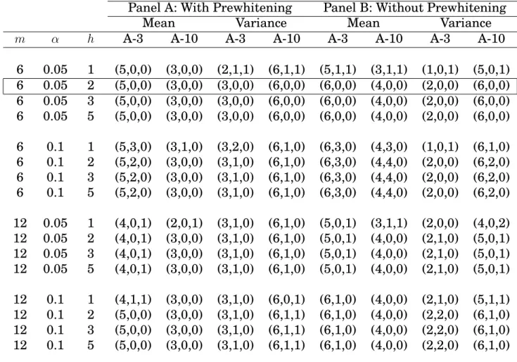
This section investigates the economics behind the differing episodes of credit spread volatility. As a measure of uncertainty, we reconstruct the eight principal components of Ludvigson and Ng (2009), who investigate the predictability of bond
risk premia, and replicate the set of macro fundamentals of Goyal and Welch (2008), who investigate the predictability of equity risk premia.
We find that our volatility factor is strongly linked to systematic forces driving both bond and equity risk premia. Across different ratings and graphs, the volatil-ity factor is closely related to the eight factors of Ludvigson and Ng (2009), with an average adjusted R-squared value of 30% (Table 1). The relation is even stronger when we use Goyal and Welch’s (2008) factors, where the average adjusted R-squared value is more than 60%. This result is meaningful because it validates results in the prior literature linking the equity premium to credit spreads (Jagannathan and Wang (1996), Chen, Collin-Dufresne, and Goldstein (2009)). It also suggests that the volatil-ity, rather than the level, of credit spreads may be the main channel through which these two assets’ risk premiums are linked. We report detailed results in Appendix J.
[Insert Table 1 about here]
VIII. Robustness Tests
A. Model Initial Parameters
We test whether the choice of initial parameters has a significant effect on the number and location of detected shifts. The key set of parameters is (m; ; h) ; where m is the initial cut-off length, is the significance level for detected shifts, and h is the Huber parameter controlling for outliers. We use the 3-, and 10-year credit spreads from the NAIC datatset and repeat the analysis by allowing the initial parameter set (m; ; h)
to take on different reasonable values and report changes in the number and location of new detected shifts: The base case applied in this study corresponds to the case where m = 6; = 5%; and h = 2: We increase the initial cut-off length from 6 to 12 months and for each parameter m; we vary the significance level between 5% and 10% and the Huber parameter h between 1 and 5. We report the triplet (shifts unchanged, shifts added, shifts dropped) in Table 2, Panel A. Unchanged shifts count the number of shifts (i.e., obtained with the new parameter set (m; ; h)) detected in the same locations or in plus or minus one month around the same locations of shifts detected in the base case. Added shifts count the number of shifts located outside shift locations of the base case and dropped shifts count the number of shifts detected in the base case but not detected in the new case. In other words, the dropped shifts count the difference between the total number of shifts detected in the base case and the number of unchanged shifts in the new case.
[Insert Table 2 about here ]
Overall, our results are robust and can be summarized as follows. First, when data values are higher than h standard deviations, they are considered outliers and are then weighted inversely proportionally with their distance from the mean value of the new regime: weight = min (1; h = ) : When the cut-off length is m = 6 and the confidence level is = 5%, the critical difference between the regimes is = 1:29 ; which leads to weight = 0:78 when h = 1. As the initial cut-off length and/or the confidence level increase, weight converges to its limit value of one and the results remain the same for different values of h. Panel A of Table 2 shows that the number
and location of the shifts for different cut-off lengths remain unchanged with h 2. Thus, our choice of h = 2 is reasonable.
Second, as the cut-off length increases, the degree of freedom increases and the value of becomes smaller, which translates into higher values of anomalies (RSI) when the regimes are longer than m: We may then detect more shifts with lower mag-nitudes. However, regimes shorter than the cut-off length can pass the test only if the magnitude of the shift is high. By increasing the size of the initial cut-off length, we account for more shifts in the case of three-year credit spreads, for example. How-ever, at least four shifts out of five (detected in the base case) remain unchanged. This confirms that the shifts for the mean value of three-year A spreads are determined correctly. Furthermore, the detected regimes for the 10-year credit spread remain the same when we increase the parameter m for h 2:
Third, the lower the confidence level, the higher and the lower the value of anomalies (RSI); which leads to a lower number of shifts. As shown in Panel A of Table 2, for a fixed m; when increases from 5% to 10%, the number of shifts added increases in several cases.
The variance ratio of two successive variance regimes depends on the critical value F ( 1; 2; ): When m = 6 and = 5%; we have F = 5:05: This means that to detect a
potential new shift in the variance, the new variance regime should be at least 5:05 times higher (lower) than the current variance regime if the shift is up (down). As the value of the initial cut-off length increases, the degrees of freedom increase and the value of F decreases for the same confidence level : In this case, we allow for more shifts to be detected if they pass the test. This has the same effect as an increase in
the confidence level, which also decreases the value of F: Panel A of Table 2 shows how the number of shifts added is different from zero as m and/or increase.
B. Effect of Red Noise
We apply the regime shift detection technique to the data without prewhitening and report our analysis for the sensitivity of detected shifts to model initial parameters in Panel B of Table 2.
As expected, the base case shows that the prewhitening procedure (Panel B of Table 2) reduces the magnitude and the number of shifts detected. In addition, we observe that red noise increases the number of detected shifts as we consider alter-native parameterizations. These results support the conclusion of Rodionov (2006).
C. Effect of the Benchmark Choice for the Risk-Free Curve
We test whether our results hold if the benchmark for the risk-free rates changes. Thus, we use the CMT bonds published by the Fed as an alternative measure for risk-free rates. Similar to corporate bond yield curves, we obtain the CMT yield curves using the Nelson–Siegel–Svensson algorithm. We repeat the regime shift detection analysis using the sample from the NAIC database.
By replacing the benchmark for the risk-free curve, we shift our credit spread curves by approximately a constant and indeed we detect similar breakpoints.
D. Using Aggregate Data
Most studies use one of the three databases described previously (Section III). How-ever, when studying the behavior of corporate bond spreads, it is preferable to have a sufficiently long time series covering several business cycles. In the current state of the literature, there is no such data source. Because our detection method is in real time, it should not be sensibly affected by a shorter sample. However, for ro-bustness, we also report the results obtained with an aggregate dataset. We join the quoted prices from the Warga and Bloomberg datasets to cover the same three re-cessions.15 Our results remain robust with respect to issues of stationarity and the
heteroskedasticity of the residuals. The level and volatility regimes only partially coincide and their patterns are in good agreement with previous results using three subperiods from the Warga, NAIC, and TRACE datasets (see Appendix K).
IX. Conclusion
Our research detects and analyzes both the level and volatility regimes in credit spreads separately, using a new random regime shift detection technique. The tech-nique is an exploratory rather than a confirmatory approach and does not require
15The Bloomberg dataset spans from March 1992 to December 2009. The index is comprised of the most frequently traded fixed-coupon bonds represented by FINRA’s TRACE. In unreported tests (available upon request), we find that the best attachment point in the overlapping period (March 1992 to December 1996) between the Bloomberg and Warga datasets is in May 1994 (for most matu-rities). Using the filtered aggregate data, we also reject the null of a unit root and find no significant autocorrelation of the residuals.
any prior assumptions about the number and timing of the regimes. We find both the level and volatility effects to be significantly distinct in their respective patterns and in their relation to the NBER cycle. High-level regimes coincide only partially with high-volatility regimes. Whereas our analysis demonstrates that recessions are accompanied by a long-lived level effect on credit spreads, the volatility effect is, in contrast, short lived. We also detect high-volatility regimes outside of NBER reces-sions, which are associated with significant financial crises, consistent with associat-ing volatility regimes with periods of high uncertainty.
We relate the credit spread cycles that we detected to the main theoretical frame-works proposed in the literature. While structural equilibrium models generate some of the detected patterns of credit spread dynamics (i.e., the countercyclicality of credit spreads, the short default episodes outside recessions, and the persistence of credit spreads), other theoretical frameworks, such as the role of monetary policy and shocks in the credit supply, can be invoked to match specific detected features (i.e., the per-sistence of credit spreads, as well as their ability to predict economic downturns). We corroborate the importance of these additional factors by applying our regime detec-tion technique to the time series of the Fed funds rate and the SLO Survey data. Our results further show evidence linking the volatility factor to important macro fundamentals that are widely accepted as predictive sources of asset risk premia.
Another potentially important determinant of credit spread dynamics, unexplored in this paper, is credit market sentiment. Buraschi, Trojani, and Vedolin (2011) de-velop a model in which agents disagree about firms’ future cash flows and future macroeconomic conditions. The heterogeneity in beliefs increases during recessions,
raising credit spreads and their volatility. As an avenue for future research, one could apply our regime detection technique on proxies for credit market sentiment, thereby gauging its empirical impact on credit spread dynamics.
References
Alexander, C., and A. Kaeck. “Regime Dependent Determinants of Credit Default Swap Spreads.” Journal of Banking and Finance, 32 (2007), 1008–1021.
Bai, J. “Common Breaks in Means and Variances for Panel Data.” Journal of Econo-metrics, 157 (2010), 78–92.
Bai, J., and P. Perron. “Estimating and Testing Linear Models with Multiple Struc-tural Changes.” Econometrica, 66 (1998), 47–78.
Bai, J., and P. Perron. “Computation and Analysis of Multiple Structural Change Models.” Journal of Applied Econometrics, 18 (2003), 1–22.
Bernanke, B., and M. Gertler. “Agency Costs, Net Worth, and Business Fluctuations.” American Economic Review, 79 (1989), 14–31.
Bhamra H. S.; A. J. Fisher; and L. A. Kuehn. “Monetary Policy and Corporate De-fault.” Journal of Monetary Economics, 58 (2011), 480–494.
Bhamra, H. S.; L. A. Kuehn; and I. A. Strebulaev. “The Levered Equity Risk Pre-mium and Credit Spreads: A Unified Framework.” Review of Financial Studies, 23 (2010), 645–703.
Buraschi, A.; F. Trojani; and A. Vedolin. “Economic uncertainty, disagreement, and credit markets.” Working paper, London School of Economics (2011).
Campbell, J. Y., and J. H. Cochrane. “By Force of Habit: A Consumption-Based Ex-planation of Aggregate Stock Market Behavior.” Journal of Political Economy, 107 (1999), 205–251.
Chen, H. “Macroeconomic Conditions and the Puzzles of Credit Spreads and Capital Structure.” Journal of Finance, 65 (2010), 2171–2212.
Chen, G.; Y. Choi; and Y. Zhou. “Nonparametric Estimation of Structural Change Points in Volatility Models for Time Series.” Journal of Econometrics, 126 (2005), 79–114.
Chen, L.; P. Collin-Dufresne; and R. S. Goldstein. “On the Relation Between the Credit Spread Puzzle and the Equity Premium Puzzle.” Review of Financial Studies, 22 (2009), 3367–3409.
Chen, N. F. “Financial Investment Opportunities and the Macroeconomy.” Journal of Finance, 46 (1991), 529–554.
Chib, S. “Estimation and Comparison of Multiple Change Point Models.” Journal of Econometrics, 86 (1998), 221–241.
Collin-Dufresne, P.; R. S. Goldstein; and J. S. Martin. “The Determinants of Credit Spread Changes.” Journal of Finance, 56 (2001), 2177–2208.
David, A. “Inflation Uncertainty, Asset Valuations, and the Credit Spread Puzzle.” Review of Financial Studies, 21 (2008), 2487–2534.
Davis, R.; T. Lee; and G. Rodriguez-Yam. “Break Detection for a Class of Nonlinear Time-Series Models.” Journal of Time Series Analysis, 29 (2008), 834–867.
Dick-Nielsen, J. “Liquidity Biases in TRACE.” Journal of Fixed Income, 19 (2009), 43–55.
Elton, E. J.; M. J. Gruber; D. Agrawal; and C. Mann. “Explaining the rate spread on corporate bonds.” Journal of Finance, 56 (2001), 247–277.
Fama, E. F., and K. French. “Business Conditions and Expected Returns on Stocks and Bonds.” Journal of Financial Economics, 25 (1989), 23–49.
Giesecke, K.; F. A. Longstaff; S. Schaefer; and I. Strebulaev. “Corporate Bond Default Risk: A 150-Year Perspective.” Journal of Financial Economics, 102 (2011), 233–250. Gilchrist, S., and E. Zakrajšek. “Credit Spreads and Business Cycle Fluctuations.” American Economic Review, 102 (2012), 1692–1720.
Giordani, P., and R. Kohn. “Efficient Bayesian Inference for Multiple Change Point and Mixture Innovation Models.” Journal of Business and Economic Statistics, 26 (2008), 66–77.
Gomes, J. F., and L. Schmid. “Equilibrium Credit Spreads and the Macroeconomy.” Working paper, Duke University (2010).
Gordon, L., and M. Pollak. “An Efficient Sequential Nonparametric Scheme for De-tecting a Change of Distribution.” Annals of Statistics, 22 (1994), 763–804.
Goyal, A., and I. Welch. “A Comprehensive Look at the Empirical Performance of Equity Premium Prediction.” Review of Financial Studies, 21 (2008), 1455–1508. Hackbarth, D.; J. Miao; and E. Morellec. “Capital Structure, Credit Risk, and Macro-economic Conditions.” Journal of Financial Economics, 82 (2006), 519–550.
Huang, J. Z., and M. Huang. “How Much of the Corporate-Treasury Yield Spread is Due to Credit Risk?” Review of Asset Pricing Studies, 2 (2012), 153–202.
Hull, J.; M. Predescu; and A. White. “The Relationship Between Credit Default Swap Spreads, Bond Yields, and Credit Rating Announcements.” Journal of Banking and Finance, 28 (2004), 2789–2811.
Jagannathan, R., and Z. Wang. “The Conditional CAPM and the Cross-Section of Expected Returns.” Journal of Finance 51 (1996), 3-54.
Kendall, M. G. “Note on Bias in the Estimation of Autocorrelation.” Biometrika, 41 (1954), 403–404.
King, M. “Debt Deflation: Theory and Evidence.” European Economic Review, 38 (1994), 419–445.
Kiyotaki, N., and J. Moore. “Credit Cycles.” Journal of Political Economy, 105 (1997), 211–248.
Koopman, S. J.; R. Kraeussl; A. Lucas; and A. A. Monteiro. “Credit Cycles and Macro Fundamentals.” Journal of Empirical Finance, 16 (2009), 42–54.
Koopman, S. J., and A. Lucas. “Business and Default Cycles for Credit Risk.” Journal of Applied Econometrics, 20 (2005), 311–323.
Lown, C., and D. Morgan. “The Credit Cycle and the Business Cycle: New Findings Using the Loan Officer Opinion Survey.” Journal of Money, Credit and Banking, 38 (2006), 1575–1597.
Lu, Y. K., and P. Perron. “Modeling and Forecasting Stock Return Volatility Using a Random Level Shift Model.” Journal of Empirical Finance 17 (2010), 138–156. Ludvigson, S. C., and S. Ng. “Macro Factors in Bond Risk Premia.” Review of Finan-cial Studies, 22 (2009), 5027–5067.
Maheu, J. M., and T. H. McCurdy. “How Useful are Historical Data for Forecast-ing the Long-Run Equity Return Distribution?” Journal of Business and Economic Statistics, 27 (2009), 95–112.
Marriott, F. H. C., and J. A. Pope. “Bias in the Estimation of Autocorrelations.” Bio-metrika, 41 (1954), 390–402.
Mueller, P. “Credit Spreads and Real Activity.” Working Paper, London School of Economics (2009).
Orcutt, G. H., and H. S. Winokur, Jr. “Autoregression: Inference, Estimation, and Prediction.” Econometrica, 37 (1969), 1–14.
Perron, P., and Z. Qu. “Estimating Restricted Structural Change Models.” Journal of Econometrics, 134 (2006), 373–399.
Pesaran, H.; D. Pettenuzzo; and A. Timmermann. “Forecasting Time Series Subject to Multiple Structural Breaks.” Review of Economic Studies, 73 (2006), 1057–1084. Rodionov, S. N. “A Sequential Algorithm for Testing Climate Regime Shifts.” Geo-physical Research Letters, 31 (2004), L09204.
Rodionov, S. N. “Detecting Regime Shifts in the Mean and Variance: Methods and Specific Examples.” Workshop on Regime Shifts, Varna, Bulgaria, (2005) 68–72. Rodionov, S. N. “Use of Prewhitening in Climate Regime Shift Detection.” Geophysi-cal Research Letters, 33 (2006), L12707.
Stine, R., and P. Shaman. “A Fixed Point Characterization for Bias of Autoregressive Estimators.” Annals of Statistics, 17 (1989), 1275–1284.
Stock, J. H., and M. Watson. “New Indexes of Coincident and Leading Economic Indicators.” NBER Macroeconomics Annual, 4 (1989), 351–409.
Wu, L., and F. X. Zhang. “A No-Arbitrage Analysis of Macroeconomic Determinants of the Credit Spread Term Structure.” Management Science, 54 (2005), 1160–1175.
Figure 1: Times Series of Credit Spreads and the Fed Funds Rate.
We plot the time series of 10-year credit spreads (left-hand side axis) and the Fed funds rate (right-hand side axis). Time is in months, credit spreads and the Fed funds rate are in percentages. The shaded regions represent NBER recessions.
Graph A : Warga Dataset from April 1987 to December 1996
Graph B : NAIC Dataset from January 1994 to December 2004
Figure 2: Time Series of Credit Spreads and the SLO Survey.
We plot the time series of 10-year credit spreads (left-hand side axis) and the SLO Survey data (right-hand side axis). Time is in months, credit spreads and the SLO Survey data are in percentages. The shaded regions represent NBER recessions.
Graph A : Warga Dataset from April 1987 to December 1996
Graph B : NAIC Dataset from January 1994 to December 2004
Figure 3: Regimes of Credit Spread Levels, Monetary Policy, and Credit Conditions. We plot detected mean regimes of 10-year credit spreads, the Fed funds rate (left-hand side axis) and the SLO Survey (right-(left-hand side axis). Time is in months, credit spreads, the Fed funds rate, and the SLO Survey data are in percentages. The shaded regions represent NBER recessions. The initial cut-off length is six months and the Huber parameter is two. All detected regimes are statistically significant at the 95% confidence level or higher.
Graph A : Warga Dataset from April 1987 to December 1996
Graph B : NAIC Dataset from January 1994 to December 2004
Table 1: Regression of the Volatility Factor on Uncertainty Variables.
We report the adjusted R-squared values from the regression of the volatility factor on the eight principal components of Ludvigson and Ng (2009) and a set of economic fun-damentals of Goyal and Welch (2008). In Goyal and Welch’s case, we omit variables causing a high variance inflation factor (i.e. V IF > 10) and those not available.
Ludvigson and Ng (2009) Goyal and Welch (2008) Warga NAIC TRACE Warga NAIC TRACE AA 0.171 0.376 0.428 0.267 0.682 0.224 A 0.284 0.382 0.197 0.409 0.622 0.681 BBB 0.318 0.303 0.248 0.324 0.719 0.752