Defining new conservation limits for Atlantic salmon (Salmo salar) populations of Brittany

Defining new conservation limits for Atlantic salmon

(Salmo salar) populations of Brittany

Clément LEBOT

Soutenu à Rennes le 14 septembre

Devant le jury composé de :

Président : Etienne Rivot (Enseignant-chercheur)

Maître de stage : Etienne Prévost (Enseignant-chercheur) Enseignant référent : Etienne Rivot (Enseignant-chercheur)

Autres membres du jury (Nom, Qualité): Guy Fontenelle (Enseignant-chercheur) Marie Nevoux (Chargée de recherché) Maxime Olmos (Doctorant)

Les analyses et les conclusions de ce travail d'étudiant n'engagent que la responsabilité de son auteur et non celle d’AGROCAMPUS OUEST

AGROCAMPUS OUEST

Année universitaire : 2016-2017

Spécialité :Sciences Halieutiques et Aquacoles

Spécialisation (et option éventuelle) : Ressources et Ecosystèmes Aquatiques

Mémoire de Fin d'Études

CFR Angers CFR Rennes

d’Ingénieur de l’Institut Supérieur des Sciences agronomiques, agroalimentaires, horticoles et du paysage

de Master de l’Institut Supérieur des Sciences agronomiques, agroalimentaires, horticoles et du paysage

d'un autre établissement (étudiant arrivé en M2)

Ce document est soumis aux conditions d’utilisation

«Paternité-Pas d'Utilisation Commerciale-Pas de Modification 4.0 France» disponible en ligne http://creativecommons.org/licenses/by-nc-nd/4.0/deed.fr

Confidentialité

si oui :

Pendant toute la durée de confidentialité, aucune diffusion du mémoire n’est possible

_.

Date et signature du maître de stage

_:

A la fin de la période de confidentialité, sa diffusion est soumise aux règles ci-dessous (droits

d’auteur et autorisation de diffusion par l’enseignant à renseigner).

Droits d’auteur

L’auteur

autorise la diffusion de son travail

Si oui, il autorise

Date et signature de l’auteur :

Autorisation de diffusion par le responsable de spécialisation ou son

représentant

L’enseignant juge le mémoire de qualité suffisante pour être diffusé

Si non, seul le titre du mémoire apparaîtra dans les bases de données.

Si oui, il autorise

Date et signature de l’enseignant :

Non Oui

1 an

5 ans

Oui Non

la diffusion papier du mémoire uniquement(4)

la diffusion papier du mémoire et la diffusion électronique du résumé la diffusion papier et électronique du mémoire (joindre dans ce cas la fiche de conformité du mémoire numérique et le contrat de diffusion)

accepte de placer son mémoire sous licence Creative commons CC-By-Nc-Nd (voir Guide du mémoire Chap 1.4 page 6)

Oui Non

la diffusion papier du mémoire uniquement(4)

la diffusion papier du mémoire et la diffusion électronique du résumé

la diffusion papier et électronique du mémoire

Résumé étendu en français

Depuis très longtemps, le saumon est présent et exploité dans les cours d’eau des façades Est et Ouest Atlantique. La France étant au Sud de son aire de répartition, les menaces pesant sur ses populations sont donc considérées comme plus importantes que dans le reste de son aire de répartition.

Le caractère anadrome de cette espèce implique une gestion imbriquée à deux échelles spatiales. Une première gestion à l’échelle des rivières qui définit l’échelle spatiale de chaque stock. La gestion à l’échelle des rivières est laissée à la charge de chaque état. Comme les individus de tous les stocks effectuent une migration commune vers les zones de nourriceries autour des Îles Féroé et au Sud du Groenland, une seconde gestion à l’échelle internationale est nécessaire. Elle est coordonnée par la NASCO qui définit les grands principes de gestion de l’espèce.

Depuis 1998, la NASCO a adopté l’approche de précaution pour gérer les populations de Saumon atlantique. Au lieu de deux points de références classiquement définis pour cette approche, à savoir une limite de conservation et une cible de gestion, à ce jour seul une limite a été définie : Sopt soit la quantité de reproducteurs qui maximise les captures à long-terme.

Ainsi, la stratégie de gestion aujourd’hui préconisée par la NASCO est une stratégie à échappement fixe (échappement correspond à Sopt) par la fixation de TAC.

En France, la gestion des populations de saumon est confiée aux comités de gestion des poissons migrateurs qui sont définis à l’échelle régionale. Elle organise la gestion en élaborant des plans de gestion des poissons migrateurs s’opérant tous les 5 ans. Néanmoins, ces plans de gestions doivent être en accord avec les recommandations définies par la NASCO. Pour s’en assurer, la NASCO exige de chaque pays un plan de mise en œuvre des grands principes établis.

Objectifs :

Dans le contexte du renouvellement de son plan de gestion des poissons migrateurs et du plan de mise en œuvre NASCO dans un futur proche, le comité de gestion Bretagne a fait savoir sa volonté de modifier la stratégie de gestion qu’elle appliquait jusqu’alors. L’objectif premier est de recentrer l’objectif des limites de conservation sur la conservation en elle-même plus que sur l’exploitation tout en intégrant certaines recommandations de la NASCO laissé de côté jusqu’à présent.

Matériels et Méthodes

La définition d’un nouveau cadre de référence pour définir les limites de conservation a été mise en place. Celui-ci est basé sur la définition de la conservation adoptée par le Canada, à savoir éviter les faibles recrutements. Deux types de références ont été utilisés pour définir ce que l’on considère comme un faible recrutement : les références théoriques issues du concept de capacité d’accueil (RMAX) et les références historiques issues du recrutement moyen (ROBS).

Le premier est défini grâce à la relation de stock-recrutement moyenne alors que le dernier utilise les données de stock-recrutement. En utilisant les différentes sources d’incertitudes autour de la relation moyenne de stock-recrutement, on a défini les limites de conservation comme le niveau de stock qui présente un risque faible de faible recrutement.

La définition de nouvelles limites de conservation concerne 18 rivières qui diffèrent les unes des autres par la taille de leur système productif ou aire d’équivalent radier-rapide. Parmi ces 18 rivières, le Scorff est une rivière atelier utilisée par le CIEM pour produire des estimations de différents stades de développement. La connaissance particulière de la dynamique de cette population nous a poussés à traiter cette rivière comme une référence.

Nous avons tiré profit des données d’indices d’abondances spécifiques à chaque rivière pour estimer des recrutements par année et rivière. Par la suite, la médiane des estimations a été utilisée comme une donnée. Pour les stocks, les médianes d’estimation de retours d’adultes sur le Scorff ont été utilisées comme des données ; pour les autres rivières, on a utilisé les captures.

Le processus d’observation reliant le stock aux captures a été rajouté à la modélisation des relations de stock-recrutement pour intégrer l’incertitude autour de ce processus. Les relations de stock recrutement ont été modélisées en moyenne par une relation de Beverton-Holt à deux paramètres en admettant une erreur log-normal autour de cette moyenne. Les paramètres standards α et RMAX de la relation de Beverton-Holt moyenne sont fixés pour le Scorff et

appliqués aux autres rivières avec un facteur multiplicatif défini pour chaque rivière r (γr).

Le modèle développé s’intègre dans la cadre de la modélisation bayésienne hiérarchique. La hiérarchisation des paramètres nous permet de créer un lien entre les rivières en tirant les paramètres de chaque rivière dans une loi de probabilité commune. Ainsi, nous pouvons transférer l’information acquise sur le Scorff aux autres cours d’eau. Le bayésien permet lui de décrire de façon complète et explicite l’incertitude utile pour définir le risque tout en nous permettant d’intégrer de la connaissance a priori sur les relations de stock-recrutement moyenne (α et RMAX).

Résultats et Discussion

Les résultats montrent un ajustement des distributions a priori sur les paramètres de Beverton-Holt. Les facteurs multiplicatifs semblent augmenter selon un gradient Est-Ouest ce qui insinue que les rivières à l’ouest de la Bretagne sont plus productives. Les relations de stock-recrutement ajustées ont permis d’évaluer les différentes limites de conservation proposées. Selon la limite de conservation, les variations entre rivières peuvent être assez importantes. Enfin, l’incertitude autour des relations de stock-recrutement est très importante. Elle est causée par l’erreur d’observation du stock, l’erreur du processus de recrutement et l’erreur d’estimation des paramètres de Beverton-Holt.

A la fin de cette étude, une discussion sur la modélisation utilisée apporte des pistes d’amélioration pour limiter le biais des limites de conservation et notamment l’introduction de co-variables pouvant expliquer les variations de captures. Enfin, nous discutons de l’application du cadre théorique développé dans cette étude à différente stratégie de gestion :

 La stratégie à échappement fixe

Table des matières

Introduction ... 1

Materials & Methods ... 4

I. Stock-recruitment relationship: a theoretical framework to incorporate uncertainty into CL definition ... 4

A. What is a Stock-recruitment relationship? ... 4

B. Using a SR curve and data to define “low recruitment” ... 5

C. Integrating the uncertainty associated to SR relationship into the definitions of CLs asdd ... 5

II. Rivers and populations of interest and available data ... 7

A. Studied populations ... 7

B. Recruitment data ... 7

C. Adult returns and spawning stock data. ... 9

III. Modeling SR relationship for rivers of Brittany to set CL. ...10

A. Outlines of the model ...10

B. Exploitation sub-model ...12

C. SR sub-model ...13

D. Bayesian framework ...14

Results ... 15

I. Diagnostics ...15

II. Exploitation sub-model ...16

A. Exploitation rates ...16

B. Adult returns ...16

III. SR sub-model ...18

A. Estimates of the SR curve parameters of the Scorff and illustration of its SR relationship ...18

B. Transferring SR relationship from the Scorff to the other rivers ...18

IV. How the CLs match with the risk diagrams and the interval of the stock level ...20

Discussion ... 22

I. Exploitation sub-model: better account for catch variability to minimize bias ...22

A. Fishing effort as a co-variable affecting the exploitation rates ...22

B. River flow as a co-variable of the exploitation rates ...23

II. Feedback on the SR sub-model ...23

A. Defining recruitment as data of YoY densities ...23

B. Feedback on the SR relationship parameters ...24

C. Addressing the issue of residual autocorrelations ...27

D. The particular case of the Aulne-Douffine River ...28

III. Establishing a dialogue with the managers to assess the relevance of the new CLs ..28

A. Being clear with the difference between CL and MT to choose between a fixed escapement strategy and the full PA ...28

B. Relevance of the new CLs given the strategy chosen ...29

References ... 31

List of illustrations

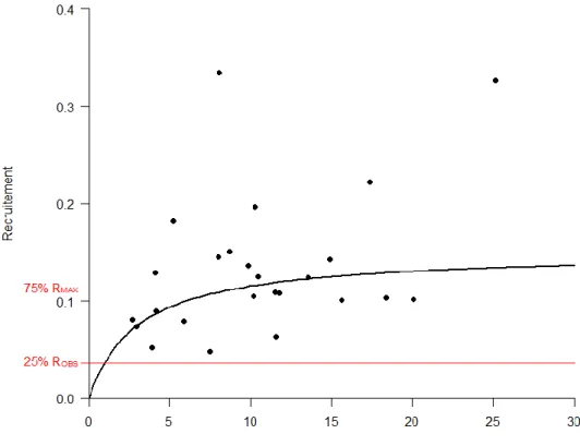
Figure 2.1. Examples of low recruitment references considered: 25% ROBS and 75% RMAX.

Figure 2.2. Examples of CL considered: CL3 and CL4. The solid line is the SR curve, which

corresponds to the evolution of the median recruitment. For any given stock level , the risk the expected recruitment falls below the SR curve is 50%. The dotted lines are analogous to the SR curve but for other risk levels, i.e. 15 % and 40%. The intersection of these curves with a pre-determined recruitment level, i.e. 75% and 25% of Rmax, allow to derive the corresponding CLs, CL3 and CL4.

Figure 2.3. Rivers of Brittany considered in this study. Rivers are figured in light blue and

sampling stations in darker blue. A number of 1 to 18 is allocated to each river according to a south-eastern to north-eastern gradient. 1: Blavet 2: Scorff 3: Ellé-Isole 4: Aven-Ster Goz 5: Odet-Jet-Steïr 6: Goyen 7: Aulne-Douffine 8: Mignonne-Camfrout-Faou 9: Elorn 10: Penzé 11: Queffleuth 12: Douron 13: Yar 14: Léguer 15: Jaudy 16: Leff 17: Trieux 18: Couesnon.

Figure 2.4. Simplified Directed Acyclic Graph of the model used. The exploitation sub-model

is figured in red whereas the SR sub-model is figured in green. Each variable and co-variable is represented with respectively an ellipse and a rectangle. When data are available, the form is shaded in grey. r is the number of river Brittany. It is included between 1 and 18. r’ is similar than r but exclude the number of the Scorff. t(r) and t(r’) illustrate the different time series available for each river.

Figure 3.1. Mean exploitation rate per river for both 1SW (left figure) and MSW (right figure). Figure 3.2. Multiplicative effects of years (left) and rivers (right).

Figure 3.3. Joint posterior distribution of the SR curve parameters of the Scorff (left) and

predictions of its SR relationship (right). In the former, prior (red) and posterior (grey) marginal distributions are presented in the marge of the figure. In the latter, shaded area represents the 95% BIC associated to each prediction of recruitment.

Figure 3.4 Multiplicative factors (left) and standard deviation (right) of every rivers.

Figure 3.5. Risk diagrams of the two references of low recruitment considered (left: theoretical,

right: historical). Each curve represents one percentage of the reference considered. 25% are represented in green, 50% in grey and 75% in red. CLs included in the prediction interval are represented.

Figure 3.6. Inter-river variability of the CLs. The left graphic shows CLs related to theoretical

references and the right graphic the CLs related to historical references.

List of tables

Table 2.1. Prior distributions of the parameters and hyper-parameters of the model

Table 3.1. Comparison between prior and marginal posterior distributions of parameter

modeled. Mean and standard deviation of the two distributions are presented. 95% BIC and median of the marginal posterior distributions are added. For variables express on another scale than natural, each estimator is index with its natural scale value.

List of appendix

Appendix 2.1. Characteristics of each river i.e. temporal trends of productive area, initial year

of recruitment time-series (all rivers have been sampled until 2016), number of stations and sampling efforts over the years.

Appendix 2.2. Modeling the observation process of the recruitment Appendix 2.3. Median recruitment time-series of every rivers of Brittany

Appendix 2.4. Sea age-specific females sex-ratio and fecundity per female (ONEMA, 2016) Appendix 2.5. Script of the model used in this study

Appendix 3.1. Median standard residual trends over the time

Appendix 3.2. Median standard residual trends in accordance to the stock levels

Appendix 3.3. Scatterplots of the 1SW exploitation rates estimates for each river and each

year

Appendix 3.4. Scatterplots of the MSW exploitation rates estimates for each river and each

year

Appendix 3.5. Scatterplots of the 1SW return estimates for each river and each year Appendix 3.6. Scatterplots of the MSW return estimates for each river and each year Appendix 3.7. Scatterplots of the stock estimates for each river and each year

Appendix 3.8. Risk diagrams used to set CL related to RMAX. Risk probability is expressed in

the y-axis and stock level in the x-axis

Appendix 3.9. Risk diagrams used to set CL related to ROBS. Risk probability is expressed in

List of abbreviations:

BCI: Bayesian confidence interval CL: Conservation limit

CL1: Stock level associated a risk of 15% to produce less 25% RMAX

CL2: Stock level associated a risk of 25% to produce less 50% RMAX

CL3: Stock level associated a risk of 40% to produce less 75% RMAX

CL4: Stock level associated a risk of 15% to produce less 25% ROBS

CL5: Stock level associated a risk of 25% to produce less 50% ROBS

CL6: Stock level associated a risk of 40% to produce less 75% ROBS

ddp: Density-dependence didp: Density-independence FET: Fixed escapement target MT: Management target PA: precautionary approach

RMAX: Carrying capacity or Maximum average recruitment

ROBS: Mean observed recruitment

SR: Stock-recruitment

Sopt: Stock level maximizing the long-term catches

RRE: Riffle-rapid equivalent

CNICS: Centre national d’interprétation des captures de salmonidés NASCO: The north Atlantic salmon conservation organization FAO: Food and agriculture organization

1

Introduction

Present and exploited in European and North-American rivers, Atlantic salmon (Salmo salar) is an emblematic species which conservation has been a matter of concern for long. Since 1996, the International Union for Conservation of Nature (IUCN) has assessed its extinction risk as lower risk / least concern (IUCN, 1996). Nevertheless, biologists and NGOs agree that its conservation is threatened in many areas within its native range (Parrish et al., 1998; WWF, 2001). The threat appears even more significant in countries at the southern edge of its distribution range as France (Verspoor, 2007).

To address A. salmon’s conservation issues, its exploitation has been regulated for a long time. However, this regulation is made difficult by the complexity of the life cycle of this species. As an anadromous fish, A. salmon reproduces in freshwater where juveniles grow before undertaking long-distance migrations in the North Atlantic Ocean, up to Sub-Artic feeding areas (Figure 1.1.). In these areas, all populations gather together and after one to three years at sea, they return to their home rivers to reproduce (Webb et al., 2007). Each river flowing into the ocean is therefore usually considered as the spatial unit associated to a salmon population, as well as the relevant spatial scale for the management of salmon stocks. At sea, salmon populations are exposed to mixed stock fisheries, so their managements required an international co-operation. In 1984, an inter-governmental organization was created: the North Atlantic Salmon Conservation Organization (NASCO). Through consultation and co-operation, NASCO assists all countries in the conservation, restoration, enhancement and rational management of salmon stocks (NASCO, 1983).

2 Following the FAO Code of Conduct for Responsible Fisheries (FAO, 1995) and the United Nations Agreement on the Conservation and Management of Straddling Fish Stocks and Highly Migratory Fish Stocks (United Nations, 1995), NASCO and its contracting parties adopted a Precautionary Approach (PA) (NASCO, 1998). It is a cautious management approach aiming at achieving conservation given the uncertainty of scientific knowledge. It requires the development of Reference Points (RP) to determine the conservation status of each population. NASCO recommends two RP: Conservation Limits (CL) and Management Targets (MT) for each salmon stock. They define three conservation status: “critical” when spawning stock are below CL, “cautious” between CL and MT and “healthy” above MT (NASCO, 1998). To define these spawning stock reference levels, we must question mechanisms driving population renewal (conservation) such as reproductive capacity and juvenile survival. They are summarized in the Stock-Recruitment (SR) relationship between the abundance of spawning stock (Stock) and the number of fish produced in the next generation and available to fisheries (Recruitment). Hence, a CL must be set at a stock level producing enough recruitment to reach population conservation. To be cautious and account for uncertainty, a management target must be significantly higher than the CL.

Presently, only CLs have been defined and used for A. salmon management (ICES, 1995). There is a wide range of options for defining the spawning stock that allows conservation (Potter, 2001). Following the International Council for the Exploration of the Sea (ICES) and United Nations advice (ICES, 1995; United Nations, 1995), NASCO recommends CLs to be set at “the spawning stock level that produces maximum sustainable yield” Sopt, commonly

known as BMSY for other marine species (NASCO, 1998). To regulate exploitation and maintain

stock above Sopt, NASCO recommends the establishment of a Total Allowable Catch (TAC)

corresponding to the number of recruits left in the population after preserving Sopt.

The management of A. salmon is operated at a national scale but must follow NASCO recommendations. Each country must provide a six-year implementation plan summarizing their management strategy. In France, the French Environmental Code entrusts the management of A. salmon to eight Regional Committees (Comité de gestion des poissons migrateurs, COGEPOMI), one of which is for Brittany. They gather various stakeholders: fishers, managers (from Governmental bodies), scientific advisors and NGOs. They define five-year management plans (PLAGEPOMI) in accordance with the French implementation plan presented to NASCO.

Brittany, holds the majority of the French A. salmon populations; i.e. about thirty. A new management strategy has been established in 1996 (Prévost and Porcher, 1996) with no major change since then. It is based on a fishing period and a Total Allowable Catch (TAC). As recommended by NASCO, the TAC is derived from the CL Sopt and defined for each river.

Once the TAC is reached, local authorities close fisheries. Note that this system essentially applies to the recreational fishery operating in freshwater (rod and line) and has little control on the estuarine and marine catches. Brittany has been a pioneer in applying this new management strategy. Later on, this was applied and adapted to other regions in France. In the context of the revision of both the new 2018-2022 management plan in Brittany and the new French implementation plan in 2019, the COGEPOMI of Brittany identified the need for a profound revision of its current management strategy.

3 Several authors agree with the need to rethink about the current NASCO operational definition of conservation and how setting Sopt as CL helps to achieve it (Chaput et al., 2013; Holt et al.,

2009; Potter, 2001). By choosing Sopt as conservation’s reference point, management of A;

salmon aims at preserving at least stock level maximizing long-term catches. Exploitation becomes central in this definition while conservation itself appears as almost subsidiary. Below Sopt, besides potential conservation issues, the main concern of managers was the decrease

in exploitation potential. Hence, current CL definition holds an ambiguity between exploitation optimization and conservation status. Moreover, the determination of Sopt requires the

construction of an equilibrium yield curve which is derive from a classical stage-to stage SR relationship. Unobserved recruitment available to fisheries is estimated by making strong hypothesis on marine survival (i.e. natural survival and fishing mortality) (Chaput et al, 2013). Marine catches affecting a single stock are usually poorly known, because of both partial reporting and mixed stock fisheries. As a result, recruitment estimates may therefore be biased as well as CL definitions.

In addition, many recommendations made by the NASCO Guidelines for the Management of

Salmon Fisheries (NASCO, 2009), are barely integrated into the current French CLs. As

recommended by NASCO (2009): “river specific CLs should be established based on data derived from each river”. But to estimate CLs, the modeling of SR relationship currently used assumes that stock and recruitment per unit of productive area is homogeneous among rivers. A unique SR relationship, drawn from the SR data and productive area of the Scorff, is readily extrapolated to the other rivers knowing their productive areas. This assumption is questionable given the variability of exposition to anthropogenic pressures and environmental conditions among rivers. NASCO (2009) encourages also that: “the management measures introduced should take into account the uncertainties in the data used » wether due to recruitment variability intra-population or to random measurement errors in the SR data (estimates). To do so, NASCO recommends to set a second reference point MT, significantly higher than CL. Given no particular approach has been recommended by neither NASCO nor ICES, no country has implemented MTs so far and uncertainty remains essentially ignored by most management strategies.

The ultimate objective of this Master’s project is to propose a new definition and practical implementation of CLs for rivers of Brittany, integrating river specific data and associated uncertainty while shifting management objective toward conservation rather than exploitation. Although focusing on Brittany Rivers, the new CLs are developed with the aim of being generalized at a broader scale, i.e. France or Europe. This work has been inspired by the recent review of Canadian PA for A. salmon management, which defines conservation as simply avoiding low recruitment (Chaput, 2015; Chaput et al., 2013; DFO, 2009).This study has been developed within the framework of the RENOSAUM project carried out in collaboration by the “Agence Française pour la Biodiversité” (AFB), the “Université de Pau et des Pays de l'Adour” (UPPA) and the “Institut National de la Recherche Agronomique” (INRA). Several CL options are proposed considering different interpretations and concrete translations of the term “low recruitment”. Uncertainty is accounted for by working on the probability of avoiding “low recruitment”. SR relationship are specifically adjusted for each river by taking advantage of the river specific data available i.e. catches and juveniles (young of the year) abundances indices. To avoid assumptions on marine survival, we consider recruitment at a freshwater stage (young of the year). Both stock and recruitment are standardized by corresponding productive areas. Joint SR modeling of all rivers is carried out through a Bayesian hierarchical model (BHM) proved useful for SR meta-analysis by borrowing strength between data rich and data poor rivers (Chaput, 2015; Liermann and Hilborn, 1997; Michielsens and McAllister, 2004; Myers, 2001; Prévost et al., 2003). SR modeling is undertaken by setting the Scorff as a reference because the long term and comprehensive survey operated on this river provides the longest and most precise time series of stock and recruitment data for Brittany.

4

Materials & Methods

I. Stock-recruitment relationship: a theoretical framework to

incorporate uncertainty into CL definition

A. What is a Stock-recruitment relationship?

As described by Walters and Korman (2001), the SR relationship must be taken “not as a curve, but rather as a family of probability distributions, with means and variances that are dependent on spawning biomass (i.e. stock). According to this definition, a curve connecting the means or modes of such distributions is called a SR curve.” Two types of factors drive the SR relationship:

 The density-dependent (ddp) factors: They are generated by windows and bottlenecks occurring mostly during the freshwater part of the A. salmon life cycle, i.e. the reproduction (Beard and Carline, 1991) and the early stages (Gibson, 1993). Negative effect of density is often referring to intraspecific competition (resources, reproduction etc), predation or parasites exposure (Elliot, 2001). Their incidence grows as the spawning stock level increases. Conversely, a positive effect of density (Allee effect) may occur at low stock levels (Elliot, 2001). Benefit of density arise from increasing probability to find mates and improve escapement to predation in condition of saturation of predators. Quite often, evidence of positive density dependence remains elusive by the sole analysis of SR data (Myers et al., 1995; Liermann and Hilborn, 1997). Only negative effects of the density-dependent factors are considered in our study.

 The density-independent (didp) factors: They refer to environmental variables defining A. salmon habitat (depth, flow, substrate or food availability). They affect A. salmon populations mostly during extreme events like winter floods or summer droughts (Elliot, 2001).

Many formulations of SR curve and associated uncertainty exist and illustrate various ecological views of the effects of ddp and didp factors on SR survival. Here, the Beverton-Holt function is used for the SR curve as increasing evidence argue in favour of its relevance for A. salmon ((Michielsens and McAllister, 2004; Pulkkinen et al., 2013). The variability surrounding SR curve is assumed to be log-normally distributed (Peterman, 1981; Shelton, 1992; Crittenden, 1994; Bradford, 1995; Walters and Korman, 2001; Prévost et al., 2003).

SR relationship are used to derive CLs based on our definition of conservation i.e. avoiding “low recruitment”. We take advantage of the SR curve and data to propose different definitions of what could be considered as “low recruitment”. Uncertainty is thereafter considered to define stock levels that allow to avoid low recruitment with various probability levels.

5

B. Using a SR curve and data to define “low recruitment”

For every river, we propose to define « low recruitment » by using two types of references:  Theoretical references: They rely on the SR curve and are derived from the carrying

capacity (RMAX). It is defined as the maximum of the average recruitment abundance that

can be supported by a given environment (Elliot, 2001). In good environmental conditions, recruitment can be higher than RMAX in some years, but on average over long term, it would

never exceed it. For the conservation of a population, it cannot be done any better than to preserve spawning stock size that would produce RMAX. In the framework of a

Beverton-Holt function, such a stock size does not exist (it would be infinite). In addition, whatever the spawning stock size, maximizing average recruitment is a goal that can be achieved at best with a 50% probability. Therefore, choosing RMAX as a reference level for defining low

recruitment appears as overly ambitious. Nevertheless, RMAX remains a useful theoretical

benchmark for recruitment. So, we propose to define “low recruitment” as a percentage of RMAX: and illustrate the approach by choosing 25, 50 and 75% (see figure 2.1. for

examples).

 Historical references: They are based on past observed SR data. Assuming a good conservation status for a given river, a low recruitment could be defined relative to the mean of the observed recruitment (ROBS). The approach is illustrated by using three

definitions of “low recruitment”: 25% ROBS, 50% ROBS and 75% ROBS (Figure 2.1.).

C. Integrating the uncertainty associated to SR relationship into

the definitions of CLs

For a given SR model, two main sources of uncertainty affect the SR relationship i.e. the uncertainty of SR observations or observation error and the uncertainty of the recruitment process. The former is due to the fact that both the stock and recruitment are not directly observed and exactly known, but rather estimated from indirect or partial observation data. The latter refers to the random variations of recruitment for any given spawning stock level. As only a couple of SR observations are available, the estimates of the parameters of the SR model (i.e. governing the SR curve and the variance of the lognormal process error) is also uncertain and produces the last source of uncertainty.

Observation error, process error, and estimation error of SR model parameters are considered for the definition of CL. For any given spawning stock, we consider the probability that a low recruitment could be produced by integrating over the above three sources of uncertainty. For instance, for a given S value, we calculate the probability that the corresponding recruitment could fall below 50% RMAX, by integrating over the recruitment process error, the estimation

error of the SR model parameters, the latter being itself derived by taking into account that SR series are also affected by some estimation error. By doing so we calculate the risk of low recruitment integrated over the main sources of uncertainty of the SR relationship.

Such calculation allows to derive plots of risk of low recruitment as a function of the stock level, low recruitment being defined beforehand. On such a plot, one can identify spawning stock levels that have an acceptable risk of low recruitment. Following Chaput et al. (2013), we define CLs on this basis. We illustrate the approach by considering several CL options corresponding to varying risk levels associated to different definitions of low recruitment. By assuming higher acceptable risk for more stringent definitions of low recruitment, we retained the following options: risk of 15% to produce 25% of RMAX (CL1) and ROBS (CL4), risk of 25% to produce 50%

of RMAX (CL2) and ROBS (CL5) and Risk of 40% to produce 75% of RMAX (CL3) and ROBS (CL6)

6

Figure 2.1. Examples of low recruitment references considered: 25% ROBS and 75% RMAX.

Figure 2.2. Examples of CL considered: CL3 and CL4. The solid line is the SR curve, which

corresponds to the evolution of the median recruitment. For any given stock level , the risk the expected recruitment falls below the SR curve is 50%. The dotted lines are analogous to the SR curve but for other risk levels, i.e. 15 % and 40%. The intersection of these curves with a pre-determined recruitment level, i.e. 75% and 25% of Rmax, allow to derive the corresponding CLs, CL3 and CL4

7

II. Rivers and populations of interest and available data

A. Studied populations

Among the thirty rivers of Brittany in which A. salmon populations are managed, only the main eighteen are considered. They are distributed along of the coast of Brittany from the south-eastern (Blavet) to the north-eastern (Couesnon) (Figure 2.3.). Rivers sharing a common estuary or with a high spatial proximity - namely the Ellé and the Isole, the Aven and the Ster Goz; the Odet, the Jet and the Steïr, the Aulne and the Douffine and the Mignonne, the Camfrout and the Faou - are pooled together and considered as a single river.

Each river is characterized by its water surface area favorable to juvenile production or productive area, expressed in m2 _{of riffles-rapids equivalent (RRE) (Bagliniere and}

Arribe-Moutounet, 1985; Bagliniere and Champigneulle, 1982; Prévost and Porcher, 1996) and accessible to A. salmon. Since 1994, it is computed thanks to riverine habitat cartography. These cartographic data are regularly updated and provide time-series of productive areas up to 2015 (Appendix 2.1.). Across rivers and years, productive areas vary by a factor of 1 to 20. The Yar and Goyen offer the smaller productive areas (about 50 000 m2 _{of riffles-rapids area)}

whereas the Ellé-Isole and Blavet have 350 000 and 650 000 m2 _{RRE available for juvenile}

production.

The Scorff is a reference river for Brittany. Its A. salmon population has been studied and monitored extensively and for a long time. It belongs to the set of index rivers used by ICES to assess the status of the species annually over its entire distribution range (ICES, 2014). It is also used by the COGEPOMI of Brittany as its reference for setting CLs and TACs for the other rivers. Its main stem is 75 km long and its drainage basin is 480 km2 _{(Baglinière and}

Champigneulle, 1986). It flows into the Atlantic Ocean at Lorient and offers a productive area to juvenile of about 200 000 m2_{. It is of intermediate size in the set of the rivers of Brittany}

considered herein. Its A. salmon adult returns and juvenile production have been continuously surveyed since the 90’s. Given its unique status, the Scorff is used as a reference further in our analyses.

B. Recruitment data

Juvenile abundance indices (AI) are collected in the Scorff since 1993 (24 years up to 2016) (Appendix 2.1.). By electro-fishing shallow running water at the beginning of autumn, the sampling protocol targets the 0+ parr or Young-of-the-Year (YoY). About fifty electro-fishing sites are sampled every year according to an accurate protocol (Prévost and Baglinière, 1995; Prévost and Nihouarn, 1999). A significant sampling effort of about 2.5 stations per 10 000 m2

of RRE is undertaken in this river.

Other rivers of Brittany

In the other rivers, IA are also collected. Time-series vary between rivers from 5 years (2012-2016) for the Mignonne-Camfrout-Faou River to 23 years (1994-(2012-2016) for the Odet-Jet-Steïr. Sampling efforts are lower than the Scorff, at an average of 1.2 stations per 10 000 m2 _{of RRE.}

8

Figure 2.3. Rivers of Brittany considered in this study. Rivers are figured in light blue and sampling stations in darker blue. A number of 1 to 18

is allocated to each river according to a south-eastern to north-eastern gradient. 1: Blavet 2: Scorff 3: Ellé-Isole 4: Aven-Ster Goz 5: Odet-Jet-Steïr 6: Goyen 7: Aulne-Douffine 8: Mignonne-Camfrout-Faou 9: Elorn 10: Penzé 11: Queffleuth 12: Douron 13: Yar 14: Léguer 15: Jaudy 16: Leff 17: Trieux 18: Couesnon

9

From data to river scale estimates of recruitment

To derive recruitment estimates at the river scale, homogenous across rivers, IA data were processed by a slightly modified version of the statistical model designed by Servanty and Prévost (2016). This model is used to estimate YoY population size and densities (per m² RRE) in the Scorff. It could not be readily generalized to all rivers of Brittany as it uses river flow as a co-variable in a way that is hard to standardize across rivers. A simplified model, but with a hierarchical setting(Appendix 2.2.), was built to jointly treat IA data of all rivers, including the Scorff.

Time-series of recruitment

In further analyses, point estimates (i.e. posterior medians) of YoY density at the river scale are used as recruitment data. No measurement errors are integrated. The time-series of recruitment are presented in the Appendix 2.3. Between rivers, recruitment varies within a wide range of variation i.e. from 0.005 YoY per m2 _{of RRE for the Aulne-Douffine in 1998 to 87}

for the Queffleuth in 2011. Within rivers, variations of recruitment can be as wide as between rivers (see Queffleuth). Compared to the other rivers, the Aulne-Douffine has the lowest average recruitments, about 0.10 YoY per m2 _{of RRE. Time-series trends are observed for 5}

rivers, i.e. an increase of YoY densities for the Scorff, the Elorn, the Penzé and the Couesnon and a decrease for the Yar.

C. Adult returns and spawning stock data.

Since 1994 and the installation of a trapping device at the head of tide, the “Moulin des Princes” station (Pont-Scorff), adults returns are assessed by capture-mark-recapture (Servanty and Prévost, 2016). A few scales are removed from each fish sampled for ageing. This allows to produce yearly estimates of one sea winter (1SW) and multi-sea winter (MSW) returns separately. Servanty and Prévost (2016) designed a statistical model for estimating annually adult by sea age category. Combined with the catch figures by sea age category obtained from the “Centre National d’Interprétation des Captures de Salmonidés” (CNICS), the spawning escapement is also estimated. The resulting time series of point estimates (posterior medians) of adult returns and spawning escapement are further used as data in this study. Given the difference of reproductive capacity between 1SW and MSW, spawner abundances are combined to derive a number of (potentially) spawned eggs. It is computed by summing the number of eggs spawned by each sea age category obtained by multiplying spawner numbers with their corresponding average proportion of females sex ratio and fecundity per female (Appendix 2.4.) Finally, numbers of eggs are expressed in density per m² of RRE using the known productive areas.

Other rivers of Brittany

For the other rivers, only catches from the CNICS are available to estimate adult returns and spawning escapement. A specific model described in the sequel (Materiel & methods III.B) has been designed to this end. Note that this model is also used to estimate adult returns of the Scorff generating the recruitment of 1993 and 1994, using the catches of 1992 and 1993 from the CNICS database.

In the Aulne-Douffine and the Elorn, video-counting devices have been installed at the lower end of each river. In the Elorn, adult returns are available since 2007 and used as observed data like for the Scorff. For the Aulne-Doufine, adult returns are available since 1999 and used as censored data because fish can by-pass the video-counting device.

10

III. Modeling SR relationship for rivers of Brittany to set CL.

A. Outlines of the model

1. Exploitation sub-model

Apart from the Scorff, there is no stock data available. Only catches provide information about the spawning adult abundance of each river. Thus, before modeling SR relationships, we modeled the observation process linking the stock to the catches (C) using an exploitation sub-model (Appendix 2.5.). Its simplified Directed Acyclic Graph (DAG) is presented figure

2.4.. In this sub-model, the link is modeled thanks to the adult returns (N) and their

corresponding exploitation rates (F). We integrate the Scorff into the modeling to take full advantage of its available data on both the stock and the catches. Unlike the recruitment, this model allows to integrate the error associated to the indirect observation of the stock into the SR modeling (SR sub-model).

2. SR sub-model

The SR sub-model is spatially structured and considers the Scorff separately from the other rivers (Figure 2.4.). Recruitment and stock data are used to model its specific SR relationship. The SR curve (median recruitment) is modeled using a Beverton-Holt function as several publications argue its relevance for A. salmon (Michielsens and McAllister, 2004; Pulkkinen et al., 2013). Two parameters are considered for the SR curve: maximum survival (α) and carrying capacity (RMAX). Like many authors, we assume the error of the recruitment process to be

log-normally distributed (Chaput, 2015; Michielsens and McAllister, 2004; Prévost et al., 2003; Pulkkinen et al., 2013; Walters and Korman, 2001).

Other rivers

For the other rivers, the same formulation of the SR curve and process error are used. To make other rivers benefit from the knowledge acquired from the Scorff, we express each SR curve relative to the SR curve of the Scorff. That is, we use the same parameters (i.e. α and RMAX) and weighted them with a multiplicative factor (δr) specific to each river. Finally, we

define the variability of the recruitment process at a river scale (σr).

3. BHM framework

Both sub-models use a hierarchical structure to transfer to any given river to the knowledge gained from all the others (Liermann and Hilborn 1997; Myers 2001; Prévost et al. 2003; Michielsens et McAllister 2004; Chaput, 2015). In particular, hierarchical modelling is applied to the exploitation rates, the multiplicative factors and all the variance parameters (Gelman, 2006).

We take advantage of the Bayesian framework to set a full probabilistic model and provide an accurate description of the uncertainty. In addition, it allows us to integrate prior knowledge on the parameters of the SR curve which can be difficult to estimate using SR data only (Walters and Korman, 2001)

11

Figure 2.4. Simplified Directed Acyclic Graph of the model used. The exploitation sub-model

is figured in red whereas the SR sub-model is figured in green. Each variable and co-variable is represented with respectively an ellipse and a rectangle. When data are available, the form is shaded in grey. r is the number of river Brittany. It is included between 1 and 18. r’ is similar than r but exclude the number of the Scorff. t(r) and t(r’) illustrate the different time series available for each river.

12

B. Exploitation sub-model

We model the observation process of the stock by means of a hierarchical model based on a theoretical variable: the density of adult returns (Dreturn). It represents the abundance of returning adults standardized by, i.e. relative to, the river size. We assume it follows a log-normal distribution with a mean (µDreturn) for each river r and year t and a single standard

deviation (σ Dreturn) common to all rivers (1).

log(Dreturn _r,t) ~ Normal (µ_Dreturn

r,t,σDreturn) (1)

Multiplicative year (ψt) and river (ρr) effects are combined to set the mean adult return (2).

µ_Dreturn

r,t = ψt × ρr (2)

Year and river effects are hierarchically modeled according to log-normal distributions. log(ψt) ~ Normal (µψ,,σψ) (3)

log(ρr ) ~ Normal (0,σρ) (4)

µψ represents the mean density of adult returns over years and rivers (log scale). σψ and σρ

are the standard deviations of the year effect and the river effect respectively.

To separate the two sea ages, we hierarchically modeled the proportion of 1SW (p1SW). It is assumed to be drawn from a beta distribution (5) reparametrized using its mean (µp1SW) and a

sample size (np1SW) (6).

p1SW_r,t ~ Beta (a,b) (5)

a = µp1SW × np1SW and b = np1SW – a (6)

Densities of each sea age are computed using the 1SW proportion (7).

D1SW r,t = Dreturn r,t × p1SWr,t and DMSW r,t+1 = Dreturn r,t × (1-p1SWr,t) (7)

Numbers of adult returns (N1SW and NMSW) are assumed to be Poisson distributed according to a parameter defined for each sea age (λ1SW and λMSW), river r and year t (8). These parameters are computed by multiplying sea age specific densities by productive areas that supported the production of the returning aduts in year t (9). Considering YoY mainly smoltify in their second year of life (Dumas and Prouzet, 2003), we use productive area of year t-2 (RREt-2) for 1SW and t-3 (RREt-3) for MSW.

N1SW_r,t ~ Poisson (λ1SW_r,t) and N1SW_r,t ~ Poisson (λMSW_r,t) (8) λ1SW_r,t = D1SW r,t × SRREt-2 and λMSWr,t= DMSW r,t × SRREt-3 (9)

Finally, both sea age catches (C1SW and CMSW) are modeled thanks to binomial laws with respectively N1SW and NMSW draws and FSW and FMSW capture probabilities (i.e. exploitation rates) (10). For each sea age, we assume exploitation rates to be normally distributed on the logit scale with one mean per river (µF1SW r or µFMSW r) and a unique standard

deviation (σF1SW and σFMSW) (11). Given exploitation rates are difficult to estimate, we used a

hierarchical structure to model mean exploitation rates. Logit-Normal distributions are used with MF1SW and MFMSW and standard deviations σµ_F1SW and σµ_FMSW (12).

C1SW_r,t ~ Binomial (N1SW_r,t ,F1SW_r,t) and CMSW_r,t ~ Binomial (NMSW_r,t ,FMSW_r,t) (10) logit(F1SW_r,t) ~ Normal (µ_F1SW

r,σF1SW) and logit(FMSWr,t) ~ Normal (µFMSWr,σFMSW) (11)

logit(µ_F1SW

13 Note that 1SW exploitation rates are set to zero for three rivers of the Morbihan (Blavet, Scorff and Ellé-Isole) in 2003 because of exceptional fisheries closure.

Finally, stock (egg density) is derived from the returns using the sea age specific catches, females sex-ratio and fecundity as well as productive areas (13).

Sr,t = (N1SWr,t-C1SWr,t)× females sex-ratio1SW× fecundity_1SW

+ (NMSW_r,t-CMSW_r,t)× females sex-ratio_MSW × fecundity_MSW) SRR⁄ _r,t (13)

C. SR sub-model

To model the SR curve, we use a Beverton-Holt function (14). It is defined according to two parameters: the maximal survival (α) and the carrying capacity (RMAX). The former is the

slope at the origin and quantifies the reproductive performance at low stock (Walters, 2001). The latter was defined in the Materiel & Methods section II.B.. A log-normal stochastic error is assigned to the recruitment process (15).

µ_R t= S_t 1 α +RS_maxt (14) Rt ~ Log-Normal (log (µR_t) ,σR) (15) Other rivers

The modeling of the SR process assumed for the other rivers is the same as for the Scorff. The SR curve parameters of the the other rivers are that of the Scorff up to a river specific multiplicative factor (δr) (16). The process error variability σ𝑅𝑟 is defined for each river (16).

µ_R r,t= ( S_r,t 1 α + Sr,t Rmax ) × δr = S_r,t 1 α_r+ Sr,t R_maxr

where αr= α × δr and R_maxr= Rmax × δr (16)

Rr,t ~ Log-Normal (log (µ_Rr,t) ,σR_r) (17)

The multiplicative factors are hierarchically modeled relative to the Scorff (multiplicative factor of 1). We assume a full exchangeability between rivers i.e. each multiplicative factors is drawn independently from the same log-normal distribution with mean µδ, and standard deviation σδ’

(log scale).

δr ~ Normal(µ_δ ,σδ') (18)

All the variance parameters (log and logit scales) are hierarchically modeled to facilitate further inferences (Gelman, 2006). The hierarchical structure is set on the precisions (τi). We used a reparametrized gamma distribution with a mean parameter (µτ) and an inverse scale (rate)

instead of a shape and a scale parameter (19).

τi ~ Gamma (shape, scale), shape = µ_τ × rate and scale = 1/rate (19) where i ∈ ⟦1:30⟧ and I = 30

14

D. Bayesian framework

All the prior distributions on the hyper-parameters and parameters are presented at table 2.1.. We set non-informative and independent priors for all hyper-parameters so that no prior distribution constrain the marginal posterior distributions.

The only exception to this general rule concern the parameters of SR curve for the Scorff. Earlier analysis with non-informative priors yielded nonsensical estimates, with much too high posterior probability associated with unrealistically high values of α or RMAX. It was thus decided

to bring some prior information to these variables by setting weakly informative priors. A beta distribution is set to α. The sample size driving the precision of the beta distribution is set to 2, to ensure the prior remains weakly informative and leave ample room for posterior updating by the data. To avoid setting to high prior probability on unrealistically high values, the maximal survival rate observed in the Scorff (4 % in 2003) is used to set By doing so, it is implicitly assumed that given the length of the series of SR observations (24 years), the maximum survival observed is (weakly) indicative of the expected survival at low stock size. Tha same rationale is used to assign a prior distribution to RMAX. An exponential distribution is used with

mean corresponding to the maximum recruitment observed in the Scorff (i.e. 0.19 YoY per m2

of RRE observed in 2003).

*_{Hyper-parameters of the model}

Table 2.1. Prior distributions of the parameters and hyper-parameters of the model Inferences

Posterior inferences and further analysis have been carried out using R and JAGS (version 4.2.0, rjags” package). The joint posterior distribution of all the unknown quantities of the model is approximated by MCMC sampling, using three chains with contrasted initial values. A posterior sample of size 15000 is obtained with a “thinning” of 10 50000 iterations per chain). The convergence of the chains is checked using the Gelman-Rubin index (Rubin and Gelman, 1992) and Geweke stationary test (Geweke, 1992). Whatever the unknown quantity, posterior statistics are derived from their marginal posterior samples (median, standard deviation and Bayesian Confidence Interval (BCI) at 95% to analyze variables). The posterior median is used as a point estimate in the sequel.

Parameter

Definition

Prior distribution

Exploitation sub-model

µψ* Equation (4) Uniform(-10,10)

µp1SW* Equation (6) Beta(1,1)

np1SW* Equation (6) Uniform(-10,10) on the log scale

MF1SW* Equation (12) Normal(0,100)

MFMSW* Equation (12) Normal(0,100)

SR sub-model

α Equation (14) Beta(0.08,1.92)

RMAX Equation (14) Exponential(0.19)

µδ* Equation (17) Uniform(-10,10) on the log scale

µτ* Equation (19) Gamma(0.1,10)

15

Results

I. Diagnostics

Convergence

We diagnose convergence of this model as upper limits of Gelman-Rubin index are lower than 1.1 and Geweke stationary test is passed for all parameters.

Prior distribution updates

Sampling in the joint posterior distribution of all the parameters updates prior distributions (Table 3.1.). Compared to the prior distributions, marginal posterior distributions are shrunk and means are modified. Note that the mean of the prior distributions of np1SW and µδ is quite

high. Indeed, uniform distributions (-10, 10) set on the log scale of the variables lead to an important density of probability for low values offset by a long tail distribution. This long tail have an important effects on estimator like the mean but no effect on other like the median (equal to 1).

Table 3.1. Comparison between prior and marginal posterior distributions of parameter

modeled. Mean and standard deviation of the two distributions are presented. 95% BIC and median of the marginal posterior distributions are added. For variables express on another scale than natural, each estimator is index with its natural scale value.

Residual analysis

To assess the fit of the model, we analyzed the standardized residuals of recruitment (Appendix 3.1.). For most of the rivers, they are normally distributed i.e. included between -1.96 and -1.96 and homogeneous between years and stock levels. Nevertheless, temporal trends appear for the Scorff and the Elorn. Residual are sensitive to the stock level in three rivers: the Penzé, the Yar and the Couesnon (Appendix 3.2.).

Parameter

Prior

Marginal posterior

Exploitation

sub-model mean sd mean sd 2.5% 50% 97.5%

µψ 0 1100 5.77 3300 -5.60 0.004 0.22 0.0001 -6.06 0.002 -5.60 0.004 -5.16 0.006 µp1SW 0.50 0.29 0.81 0.01 0.78 0.81 0.83 np1SW 1100 3300 34.07 6.33 23.43 33.51 47.99 MF1SW 0 0.5 100 0.5 -3.24 0.04 0.25 0.01 -3.75 0.02 -3.24 0.04 -2.76 0.06 MFMSW 0 0.5 100 0.5 -1.80 0.14 0.23 0.03 -2.25 0.1 -1.80 0.14 -1.34 0.21 SR sub-model α 0.04 0.11 0.03 0.01 0.02 0.03 0.07 RMAX 0.19 0.19 0.20 0.07 0.11 0.19 0.39 µδ 1100 3300 1.49 0.31 0.97 1.46 2.20 µτ 0.01 2.87 4.50 0.73 3.36 4.40 6.22 rate 0.01 2.90 0.85 0.51 0.27 0.74 2.11

16

II. Exploitation sub-model

A. Exploitation rates

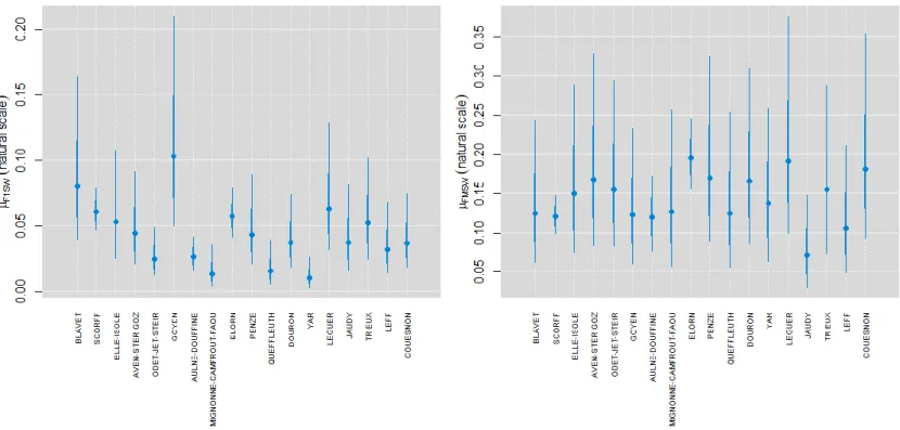
As shown in the table 3.1., the 1SW mean exploitation rates across rivers (MFSW) is

0.04% (median). As presented in the figure 3.1, for this sea age, the median exploitation rate of the Scorff is slightly higher than the other rivers (0.06%) and its estimation is sparsely variable (standard deviation of 0.008 on the natural scale). For the other rivers, the median exploitation rates vary from a factor 1 to 10. The lower median value is estimated to 0.01 for the Yar whereas the higher is estimated to 0.10 for the Goyen. The latter have the most variable estimate with a standard deviation of 0.04.

For the MSW, the mean exploitation rate across rivers (MFMSW) is estimated to 0.14%. It is

about three times higher than estimate for 1SW. For the Scorff, the mean exploitation rate is relatively smaller than mean across rivers (0.12) and its estimate is sparsely variable (0.01). For the other rivers, the mean estimates are less variable than 1SW and vary from a factor of 1 to 2.5. The lower mean is estimated for the Jaudy (0.08) and the higher for the Elorn (0.2). Estimates of MSW mean exploitation rates are generally more variable than 1SW estimates.

Finally for most of the rivers, no temporal trend on annual exploitation rates is highlighted (Appendix .3.3. and Appendix 3.4.). Note than 1SW exploitation rates seem to decrease in the Aulne-Douffine. In the Elorn, a significantly higher exploitation rate is estimated for the year 2007.

B. Adult returns

The mean density of adult returns (µψ) is estimated to 0.004.m-2 of RRE (table 3.1.)

Median year effects vary with an amplitude of ± 0.002.m2 _{of RRE around mean estimate}

density (figure 3.2.). Maximum medians are estimated for years 1995, 2004 and 2010 whereas minima are estimated in 1997 and 2009.

Random effects of rivers are shown figure 3.2.. The median vary between rivers from a factor 1 to 4. Thus, for a particular river of Brittany, median density of adult returns is included between half and twice mean adult density. The median effect of the Scorff is estimated to be a quarter lower than the other rivers (ρ2 = 0.75). For the other rivers, two trends are observed.

In the south of the Brest bay (until the Aulne-Douffine), median river effects increase along an east-west gradient. Further north, river effects are more variable with low values for rivers with productive areas smaller than 100 000m2_{(Mignonne-Camfrout-Faou, Queffleuth, Yar and Leff).}

Mean proportion of 1SW (µp1SW) is estimated to 81% (table 3.1). For the Scorff, the proportion

of 1SW in the adult returns is decreasing since the end of the 90’s. For the other rivers, the variability of the estimates is too high to detect temporal trend.

As 1SW proportion, the high variabilities of 1SW and MSW estimates hide all possible temporal trend (Appendix 6.5. and Appendix 6.6.). However, we note a slight increase over time for the Ellé-Isole, the Aven-Ster Goz and the Couesnon. The absence of adult return trends spreads to stock estimates (Appendix 6.7.).

17

Figure 3.1. Mean exploitation rate per river for both 1SW (left figure) and MSW (right figure)

18

III. SR sub-model

A. Estimates of the SR curve parameters of the Scorff and

illustration of its SR relationship

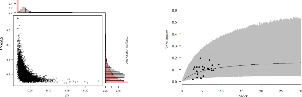
Joint posterior distribution of SR curve parameters

The marginal distribution (prior and posterior) as well as the joint posterior distribution of the SR curve parameters are presented figure 3.3. The median of the marginal distribution of is 0.03% for α and 0.19 YoY.m2 of RRE for RMAX (table 3.1.). The uncertainty of the estimates is

important for both parameters as 95% BIC bounds differ from a factor of 4 (95% BIC of α [0.02, 0.07] and RMAX [0.11, 0.39]). Their joint posterior distribution has a « banana » shape and

highlight a strong negative relationship between them. It is observed when information provided by the SR data of the Scorff is insufficient to estimate SR curve parameters independently (Walters and Korman, 2001; Bret, 2012). For the Scorff, very low stock level is not observed and as a consequence likelihoods of low and high value of α are equivalent. To fit with the data, low values of α are offset with high values of RMAX and conversely. The weakly

informative priors set on both α and RMAX prevent from extreme estimates of these variables.

SR relationship of the Scorff

In the Figure 3.3, the SR relationship of the Scorff is presented. It highlights the high uncertainty surrounding the SR curve caused by the observation errors related to the stock, the errors of the recruitment process and the errors of the estimation of SR curve parameters. These three sources of uncertainty result in an overall standard deviation of 0.58 (median on the log scale) surrounding the SR curve.

B. Transferring SR relationship from the Scorff to the other rivers

As presented in the table 3.1.., the mean multiplicative effect is estimated to 1.46 (median). The density-dependence is stronger in the Scorff than in the other rivers as its value is lower than the median multiplicative effects of most of the others rivers (Figure 3.4). Only two rivers have lower estimates multiplicative factors: the Aulne-Douffine and the Couesnon. The former have the lowest multiplicative factor equal to 0.3 corresponding to a density-dependence five times higher than average. Except the Aulne-Douffine, the medians of multiplicative factors increase along an east-west gradient and lead to a decrease of density-dependence. This result can be interpreted by a difference of geomorphology of the rivers along this gradient.

Uncertainty of recruitment process

Besides multiplicative factors estimates, Figure 3.4 presents also the estimates of standard deviation (log scale) of all the rivers of Brittany. The standard deviation estimates vary among rivers, which validate the choice of modelling a river specific variance parameter. Noted that the Queffleuth has the most uncertain recruitment process. This result was expected given the high variability of recruitment produced with similar stock levels (See Materials and Methods section II.B.).

19

Figure 3.3. Joint posterior distribution of the SR curve parameters of the Scorff (left) and predictions of its SR relationship (right). In the former,

prior (red) and posterior (grey) marginal distributions are presented in the marge of the figure. In the latter, shaded area represents the 95% BIC associated to each prediction of recruitment.

20

IV. How the CLs match with the risk diagrams and the interval of

the stock level

Scorff

To set the CLs of the Scorff, we take advantage of risk diagrams (Figure 3.5.). For each stock level, it predicts the risk that the recruitment produced will be inferior to the references. Predictions is undertaken each 0.1 stock level between 0 to 30 eggs.m-2 _{of RRE.}

Thanks to this diagram we could therefore set the propositions of CLs (see paragraph Materials and Methods I.C). The risk diagrams translate the high uncertainty of the SR relationship into the risk associated to recruitment production. Risk curves are drawn for each “low recruitment” references. For all of them, minimum risks obtained for 30 eggs.m-2 _{of RRE are higher than 0.}

Lower minimum risks associated to historical references are: 0.001, 0.03 and 0.11 for 25, 50 and 75% ROBS respectively. Theoretical references have higher minimum risks equal to 0.02,

0.2 and 0.44 for 25, 50 and 75% RMAX respectively. Thus, for too ambitious definition of “low

recruitment” as 75% RMAX the associated risk of 40% is not reached in the interval of

predictions.

For theoretical and historical references, higher the percentage considered is, higher the CLs are even if risks decrease. The theoretical CLs, CL1 and CL2 respectively associated to

25%RMAX and 50%RMAX are reached under 30eggs.m-2 of RRE. CL1 is set to 6.1 eggs.m-2 of

RRE and is included in the interval of observed stock whereas CL2 is set to 19.4 eggs.m-2 of

RRE and is two times superior to the maximum observed stock level. Compared to RMAX related

CLs, CLs using ROBS are lower and less variables. They are all lower than the maximum

observed stock levels. Their values vary from 1.9 for CL4 to 5 eggs.m-2 of RRE for CL6, CL5

being set to 3.8. Note that CL4 is lower than the minimum observed recruitment.

The other rivers

The observations established for the Scorff are generalized to the other rivers. That is, CL3 are higher than maxima of prediction intervals and must not be considered (Appendix 3.8.

and Appendix 3.9.). CL4 and CL2 are no included in the interval of observed stock whereas

CL1, CL5 and CL6 lay within the interval for most of the rivers.

Nevertheless, for some rivers, these three limits slide out from the stock interval. In the Queffleuth, the limits are relatively higher than in the other rivers (Figure 3.6.) and fall above the maximum of the median stock observed. It is mainly due to the high variability of the SR relationship (Figure 3.4.) which increase the CL values as recruitment process being more uncertain and the low and narrow stock interval. For this river, CL4 belongs to the interval of

the median stock. The inverse phenomenon is observed for CL1 and CL5 in the Goyen and the

Ellé-Isole i.e. CL1 and CL5 fall below their stock interval. For the Goyen, these two CLs are

comparable to the other rivers but the relative high stocks in this river make these CLs fall below the interval. For the Ellé-isole, it is rather due to the low standard deviation of its SR relationship that decreases the uncertainty of the recruitment process and the CL values. Despite its wide stock interval, CL1 and CL5 are too low to belong to it (Appendix 3.9.).

Within theoretical and historical references, the range of variability of the CLs becomes wider when the percentage and the risk increased. Excepted from the Queffleuth, CL1 is relatively

constant with a value of about 5 eggs.m-2 _{of RRE for each river whereas CL}

5 and CL6 varies

from 3 to 10 and from 4 to 13 eggs.m-2 _{of RRE respectively. CL}

4 and CL2 are less and more

21

Figure 3.5. Risk diagrams of the two references of low recruitment considered (left: theoretical,

right: historical). Each curve represents one percentage of the reference considered. 25% are represented in green, 50% in grey and 75% in red. CLs included in the prediction interval are represented.

Figure 3.6. Inter-river variability of the CLs. The left graphic shows CLs related to theoretical