Finite-Sample Diagnostics for Multivariate Regressions with Applications to Linear Asset Pricing Models

Texte intégral

(1)2003s-34. Finite-Sample Diagnostics for Multivariate Regressions with Applications to Linear Asset Pricing Models Jean-Marie Dufour, Lynda Khalaf, Marie-Claude Beaulieu. Série Scientifique Scientific Series. Montréal Avril 2003. © 2003 Jean-Marie Dufour, Lynda Khalaf, Marie-Claude Beaulieu. Tous droits réservés. All rights reserved. Reproduction partielle permise avec citation du document source, incluant la notice ©. Short sections may be quoted without explicit permission, if full credit, including © notice, is given to the source..

(2) CIRANO Le CIRANO est un organisme sans but lucratif constitué en vertu de la Loi des compagnies du Québec. Le financement de son infrastructure et de ses activités de recherche provient des cotisations de ses organisationsmembres, d’une subvention d’infrastructure du ministère de la Recherche, de la Science et de la Technologie, de même que des subventions et mandats obtenus par ses équipes de recherche. CIRANO is a private non-profit organization incorporated under the Québec Companies Act. Its infrastructure and research activities are funded through fees paid by member organizations, an infrastructure grant from the Ministère de la Recherche, de la Science et de la Technologie, and grants and research mandates obtained by its research teams. Les organisations-partenaires / The Partner Organizations PARTENAIRE MAJEUR . Ministère du développement économique et régional [MDER] PARTENAIRES . Alcan inc. . Axa Canada . Banque du Canada . Banque Laurentienne du Canada . Banque Nationale du Canada . Banque Royale du Canada . Bell Canada . Bombardier . Bourse de Montréal . Développement des ressources humaines Canada [DRHC] . Fédération des caisses Desjardins du Québec . Gaz Métropolitain . Hydro-Québec . Industrie Canada . Ministère des Finances [MF] . Pratt & Whitney Canada Inc. . Raymond Chabot Grant Thornton . Ville de Montréal . École Polytechnique de Montréal . HEC Montréal . Université Concordia . Université de Montréal . Université du Québec à Montréal . Université Laval . Université McGill ASSOCIÉ AU : . Institut de Finance Mathématique de Montréal (IFM2) . Laboratoires universitaires Bell Canada . Réseau de calcul et de modélisation mathématique [RCM2] . Réseau de centres d’excellence MITACS (Les mathématiques des technologies de l’information et des systèmes complexes) Les cahiers de la série scientifique (CS) visent à rendre accessibles des résultats de recherche effectuée au CIRANO afin de susciter échanges et commentaires. Ces cahiers sont écrits dans le style des publications scientifiques. Les idées et les opinions émises sont sous l’unique responsabilité des auteurs et ne représentent pas nécessairement les positions du CIRANO ou de ses partenaires. This paper presents research carried out at CIRANO and aims at encouraging discussion and comment. The observations and viewpoints expressed are the sole responsibility of the authors. They do not necessarily represent positions of CIRANO or its partners.. ISSN 1198-8177.

(3) Finite-Sample Diagnostics for Multivariate Regressions with Applications to Linear Asset Pricing Models* Jean-Marie Dufour†, Lynda Khalaf ‡, Marie-Claude Beaulieu§. Résumé / Abstract Dans cet article, nous proposons plusieurs tests de spécification valides pour des échantillons finis dans le cadre de régression linéaires multivariées (RLM), avec des applications à des modèles d’évaluation d’actifs. Nous nous concentrons sur les déviations par rapport à l’hypothèse d’erreurs i.i.d. univariée ou multivariée, pour des distributions d’erreurs gaussiennes et non gaussiennes. Les tests univariés étudiés prolongent les procédures exactes existantes en permettant des paramètres non spécifiés dans la distribution des erreurs (e.g., le nombre de degrés de liberté dans le cas de la distribution de Student). Les tests multivariés sont basés sur des résidus standardisés multivariés qui assurent l’invariance par rapport aux coefficients RLM et à ceux de la matrice de covariance des erreurs. Nous considérons des tests contre la dépendance sérielle, contre la présence d’effets GARCH multivariés et des tests de signes contre l’asymétrie. Les procédures proposées sont des versions exactes des tests de Shanken (1990) qui consistent à combiner des tests de spécification univariés. Spécifiquement, nous combinons des tests entre équations en utilisant une approche de test de Monte Carlo (MC), ce qui permet d’éviter des bornes de type Bonferroni. Étant donné que les tests dans un contexte non gaussien ne sont pas pivotaux, nous appliquons une approche de test de Monte Carlo maximisé [Dufour (2002)] où la valeur p simulée pour l’hypothèse testée (qui dépend de paramètres de nuisance) est maximisée (par rapport aux dits paramètres de nuisance) dans le but de contrôler le niveau des tests. Nous appliquons les tests proposés à un modèle d’évaluation d’actifs qui comprend un taux d’intérêt sans risque observable et utilise les rendements de portefeuilles mensuels de titres inscrits à la bourse de New York, sur des sous-périodes de cinq ans allant de janvier 1926 à décembre 1995. Nos résultats révèlent que les tests univariés exacts présentent des problèmes de dépendance * This work was supported by the Canada Research Chair Program (Chair in Econometrics, Université de Montréal), the Alexander-von-Humboldt Foundation (Germany), the Institut de Finance mathématique de Montréal (IFM2), the Canadian Network of Centres of Excellence [program on Mathematics of Information Technology and Complex Systems (MITACS)], the Canada Council for the Arts (Killam Fellowship), the Natural Sciences and Engineering Research Council of Canada, the Social Sciences and Humanities Research Council of Canada, and the Fonds FCAR (Government of Québec). This paper was also partly written at the Centre de recherche en Économie et Statistique (INSEE, Paris), the Technische Universität Dresden (Fakultät Wirtschaftswissenschaften) and the Finance Division at the University of British Columbia. † Canada Research Chair Holder (Econometrics). Centre interuniversitaire de recherche en analyse des organisations (CIRANO), Centre interuniversitaire de recherche en économie quantitative (CIREQ), and Département de sciences économiques, Université de Montréal. Mailing address: Département de sciences économiques, Université de Montréal, C.P. 6128 succursale Centre-ville, Montréal, Québec, Canada H3C 3J7. Tel: 1 514 343 2400; Fax: 1 514 343 5831; E-mail: jean.marie.dufour@umontreal.ca. Web page: http://www.fas.umontreal.ca/SCECO/Dufour. ‡ Centre interuniversitaire de recherche en économie quantitative (CIREQ), and GREEN, Université Laval, Pavillon J.-A. De Sève, St. Foy, Québec, Canada, G1K 7P4. Tel: (418) 656 2131-2409; Fax: (418) 656 7412. E-mail: lynda.khalaf@ecn.ulaval.ca. § Centre Interuniversitaire de Recherche sur les Politiques économiques et l'Emploi (CIRPÉE), Département de finance et assurance, Pavillon Palasis-Prince, local 3632, Université Laval, Québec, Canada G1K 7P4. Tel: (418) 656-2926, Fax: (418) 656-2624. E-mail: Marie-Claude.Beaulieu@fas.ulaval.ca..

(4) sérielle, d’asymétrie et d’effets GARCH statistiquement significatifs dans certaines équations. Cependant ces problèmes s’avèrent moins importants, lorsque l’on tient compte de la dépendance entre équations. De plus, les écarts importants par rapport à l’hypothèse i.i.d. sont moins évidents une fois que l’on considère des erreurs non gaussiennes. Mots clés : modèle d’évaluation d’actifs financiers; CAPM; efficacité moyenne-variance; nonnormalité; modèle de régression multivarié; hypothèse uniforme linéaire; test de Monte Carlo; bootstrap; paramètre de nuisance; test de spécification; diagnostics; GARCH; test du ratio des variances. In this paper, we propose several finite-sample specification tests for multivariate linear regressions (MLR) with applications to asset pricing models. We focus on departures from the assumption of i.i.d. errors assumption, at univariate and multivariate levels, with Gaussian and nonGaussian (including Student t) errors. The univariate tests studied extend existing exact procedures by allowing for unspecified parameters in the error distributions (e.g., the degrees of freedom in the case of the Student t distribution). The multivariate tests are based on properly standardized multivariate residuals to ensure invariance to MLR coefficients and error covariances. We consider tests for serial correlation, tests for multivariate GARCH and sign-type tests against general dependencies and asymmetries. The procedures proposed provide exact versions of those applied in Shanken (1990) which consist in combining univariate specification tests. Specifically, we combine tests across equations using the MC test procedure to avoid Bonferroni-type bounds. Since non-Gaussian based tests are not pivotal, we apply the “maximized MC” (MMC) test method [Dufour (2002)], where the MC p-value for the tested hypothesis (which depends on nuisance parameters) is maximized (with respect to these nuisance parameters) to control the tests significance level. The tests proposed are applied to an asset pricing model with observable risk-free rates, using monthly returns on New York Stock Exchange (NYSE) portfolios over five-year subperiods from 1926-1995. Our empirical results reveal the following. Whereas univariate exact tests indicate significant serial correlation, asymmetries and GARCH in some equations, such effects are much less prevalent once error crossequation covariances are accounted for. In addition, significant departures from the i.i.d. hypothesis are less evident once we allow for non-Gaussian errors. Keywords: capital asset pricing model; CAPM; mean-variance efficiency; non-normality; multivariate linear regression; uniform linear hypothesis; exact test; Monte Carlo test; bootstrap; nuisance parameters; specification test; diagnostics; GARCH; variance ratio test. Codes JEL : C3; C12; C33; C15; G1; G12; G14..

(5) Contents 1.. Introduction. 1. 2.. Framework and exact distributional theory 2.1. Exact invariance results . . . . . . . . . . . . . . . . . . . . . . . . . . . . . . 2.2. Exact Monte Carlo test procedure . . . . . . . . . . . . . . . . . . . . . . . . .. 3 4 5. 3.. Multivariate specification tests 3.1. Generalized diagnostics . . . 3.2. Joint tests for GARCH effects 3.3. Joint serial dependence tests 3.4. Sign tests against asymmetry. . . . .. 6 6 7 8 9. Empirical application 4.1. Overview of the results . . . . . . . . . . . . . . . . . . . . . . . . . . . . . . 4.2. Detailed discussion of the results . . . . . . . . . . . . . . . . . . . . . . . . .. 10 21 21. 4.. . . . .. . . . .. . . . .. . . . .. . . . .. . . . .. . . . .. . . . .. . . . .. . . . .. . . . .. . . . .. . . . .. . . . .. . . . .. . . . .. . . . .. . . . .. . . . .. . . . .. . . . .. . . . .. . . . .. . . . .. . . . .. . . . .. 5.. Conclusion. 25. A.. Appendix: Monte Carlo goodness-of-fit tests. 27. List of Tables 1 2 3. Portfolio definitions . . . . . . . . . . . . . . . . . . . . . . . . . . . . . . . . Univariate and Multivariate GARCH Tests . . . . . . . . . . . . . . . . . . . . Table: Univariate and Multivariate Predictability Tests . . . . . . . . . . . . . .. iii. 10 11 16.

(6) 1. Introduction The multivariate linear regression (MLR) model is certainly one of the most basic and widely used model in finance, econometrics and statistics in general [see Rao (1973, Chapter 8), Anderson (1984, chapters 8 and 13), Kariya (1985), Dufour and Khalaf (2002d), and the references therein]. Well known financial applications include: (i) tests of portfolio efficiency in the context of the capital asset pricing model (CAPM) [see for example: Gibbons (1982), Shanken (1986), MacKinlay (1987), Barone-Adesi (1986), Gibbons, Ross and Shanken (1989, GRS), Affleck-Graves and McDonald (1989), Shanken (1990), Zhou (1991), Zhou (1993), Zhou (1995), Fama and French (1993, 1995), Shanken (1996), Campbell, Lo and MacKinlay (1997, Chapter 5), Stewart (1997), Velu and Zhou (1999), Chou (2000), Groenwold and Fraser (2001), and Beaulieu, Dufour and Khalaf (2001b, 2001a)]; (ii) spanning tests [see Jobson and Korkie (1982, 1989) and Kan and Zhou (2001)]; and (iii) event studies [see Binder (1985) and Schipper and Thompson (1985)]. A common feature of such models consists in assuming that the disturbances (or the errors) in different equations are correlated across equations, but otherwise constitute independent identically distributed (i.i.d.) random vectors. Of course, violation of the latter assumption can affect the results of various tests and inferences based on the model (such as mean-variance efficiency or spanning tests). This underscores the importance of performing diagnostics on such multivariate models. As emphasized by Kroner and Ng (1998), the existing literature on multivariate diagnostics is sparse compared to the univariate case. Perhaps because of this, diagnostic tests in empirical MLRbased financial studies are often conducted on an equation by equation basis. Although univariate tests can provide some guidance, contemporaneous correlation of disturbances entails that statistics from individual equations are not independent. As a result, combining test decisions over all equations raises size control problems, so the need for joint testing naturally arises; see Richardson and Smith (1993) and Shanken (1990). In this context, joint diagnostics are typically based either on asymptotic approximations or on Bonferroni-type bounds. The procedures suggested following the first approach involve test statistics which formally incorporate cross-sectional dependence yet are asymptotically free of nuisance parameters; see, for example, Godfrey (1988), Richardson and Smith (1993) and the recent literature on multivariate GARCH, which may be traced back to Engle and Kroner (1995) and Kroner and Ng (1998). Although this may lead to convenient test procedures, the fact remains that crossequation correlations can still affect the null distributions of the test statistics in finite samples. In systems with many equations (e.g., many portfolios), the number of correlations can be quite large relative to the sample size, leading to serious degrees-of-freedom losses and size distortions. As a result, asymptotic approximations perform poorly in finite samples; for references and simulation evidence, see Shanken (1996, Section 3.4.2), Campbell et al. (1997, Chapter 5), and Dufour and Khalaf (2002b, 2002d, 2002c). Alternatively, Bonferroni-based bound joint tests require one to divide the significance level of each individual test by the number of tests [see Dufour (1990), Shanken (1990), Dufour and Torrès (1998), Dufour and Khalaf (2002b)]. While this can guard against spurious rejections, it can also cause severe power losses if the MLR includes many equations. Despite the above problems, very few finite sample exact specification tests have been proposed. 1.

(7) for MLR models. One exception includes work on testing the independence between the disturbances in different equations [see Harvey and Phillips (1982) and Dufour and Khalaf (2002b)]. But this problem is relatively simple, for the null hypothesis sets the error covariances to zero. The basic difficulty one meets here consists in allowing for an unknown contemporaneous covariance matrix which involves a rapidly growing number of nuisance parameters as the number of equations increases. In this paper, we consider the problem of testing the specification of MLR models. Of course, the form of a model can be tested against an infinity of alternative formulations or specification errors. Here we focus on the following basic deviations from the MLR specification: (1) detecting the presence of GARCH-type heteroskedasticity; (2) detecting (linear) serial dependence; (3) testing whether the errors follow a symmetric distribution. For these three problems, we propose procedures based on least squares residuals, hence computationally simple. In order to avoid the nuisance parameter problem raised by the unknown error covariance matrix, we apply a multivariate rescaling transformation which eliminates the unknown covariance matrix from the residual distribution. In this way, we get multivariate standardized residuals which are location-scale invariant, hence do not depend on the (unknown) regression coefficients or the error covariance matrix. The tests against the presence of GARCH effects include multivariate extensions of the univariate procedures proposed by Engle (1982), Lee (1991) and Lee and King (1993). The tests for linear serial dependence are multivariate versions of the portmanteau Ljung-Box [Ljung and Box (1978)] and variance ratio [Lo and MacKinlay (1988, 1989)] tests. For testing symmetry, we introduce a sign procedure. All these tests are applied to properly standardized residuals. None of the exact procedures is based on a Bonferroni bound, i.e. they do not require one to divide the significance level by the number of individual equations. To overcome multiple-test concerns as well as the fact that the test statistics considered have complicated null distributions which can be extremely difficult to evaluate analytically, we apply the Monte Carlo (MC) test technique [Dwass (1957), Barnard (1963), Dufour and Kiviet (1996), Dufour and Kiviet (1998)], which provides randomized exact versions of the tests considered. The MC simulation-based procedure yields an exact test whenever the joint distribution of the individual test statistics does not depend on unknown nuisance parameters (i.e., the test statistics are jointly pivotal) under the null hypothesis and general parametric distributional assumptions. The fact that the relevant analytical distributions are quite complicated is not a problem: all we need is the possibility of simulating the relevant test statistics under the null hypothesis. The combined procedures described also provide exact versions of those applied by Shanken (1990) without the need to use bounds. Furthermore, our methodology deals, from a finite-sample perspective, with non-normal errors. Formally, this allows one to test for time varying variances or asymmetries, with fat-tailed error distributions such as the Student t. This approach is new, even in the case of univariate tests. Indeed, in this case, the recent literature on simulation based testing [see e.g. Dufour, Khalaf, Bernard and Genest (2001), Dufour and Khalaf (2002a) for univariate residuals based heteroskedasticity and serial correlation tests] allows one to deal with non-Gaussian disturbances, if the error distribution is fully specified. For instance, in the case of the Student t distribution, with an unknown degreeof-freedom parameter, it will typically appear in the null distribution of the diagnostic test statistic.. 2.

(8) In the present paper, we extend the procedures proposed in Dufour et al. (2001) and Dufour and Khalaf (2002a) to account for unspecified parameters in the hypothesized error distribution. To control significance level given such difficulties, we apply a “maximized MC” (MMC) test [see Dufour (2002)], where the MC p-value for the tested hypothesis (which depends on the nuisance parameter) is maximized over the relevant nuisance parameter set.1 The procedures proposed are applied to a typical multivariate market-model based on New York Stock Exchange (NYSE) portfolios, constructed from the University of Chicago Center for Research in Security Prices (CRSP) data base for the period 1926-1995. In Beaulieu, Dufour and Khalaf (2001b), this data set is analyzed in view of testing mean-variance efficiency. Here, we assess the specification using the procedures described above. In particular, we perform finite-sample tests _ both univariate and multivariate _ of the assumption of i.i.d. errors against the presence of GARCH effects [using joint Engle and Lee-King tests] as well as against linear serial dependence [using joint Ljung-Box and variance ratio tests]. This allows us to compare and contrast evidence from both approaches. Furthermore, the sign procedure is applied to test symmetry. Our empirical results reveal the following. Whereas univariate exact tests indicate some serial correlation and GARCH effects, the multivariate tests indicate that such effects are less prevalent (at least in the time frames considered) once the cross-equation error covariances are considered. This underscores the merits of formal multivariate testing approaches. More importantly, significant departures from the i.i.d. hypothesis are less evident when we allow for non-Gaussian errors. This illustrates the importance of formally accounting for error distributions from a finite-sample perspective. The paper is organized as follows. Section 2 sets the framework and presents our basic exact distributional results. In Section 3, we present our univariate and multivariate diagnostic criteria. Section 4 reports our empirical analysis. We conclude in Section 5.. 2. Framework and exact distributional theory Many asset pricing models take the form of a system of correlated regression equations, i.e. Y = XB + U. (2.1). where Y = [Y1 , ... , Yn ] is a T × n matrix of observations on n dependent variables, X is an T × k full-column rank matrix , B = [B1 , . . . , Bn ] is a k × n matrix of unknown coefficients and U = [U1 , . . . , Un ] = [V1 , . . . , VT ]0 is a T × n matrix of random disturbances. For example, a one-factor asset pricing model can be written: rit = ai + bi reMt + uit ,. t = 1, . . . , T, i = 1, . . . , n ,. 1. (2.2). For further discussions of MMC tests in econometrics, see Dufour and Khalaf (2001, 2002c). When nuisance parameters appear in the null distribution of a test statistic, a test is exact at level α if the largest rejection probability over the nuisance parameter space consistent with the null hypothesis is not greater than α [see Lehmann (1986, sections 3.1, 3.5)].. 3.

(9) e Mt − RtF , Rit is the returns on security i for period t, R e Mt are the where rit = Rit − RtF , reMt = R F returns on the market portfolio under consideration, Rt is the riskless rate of return (i = 1, . . . , n, t = 1, . . . , T ), and uit is a random disturbance. Clearly, this model is a special case of (2.1) where Y ιT. = [r1 , ... , rn ] , 0. = (1, . . . , 1) ,. ri = (ri1 , ... , riT )0 ,. X = [ιT , reM ] , 0. reM = (e rM1 , . . . , reMT ) ,. Ui = (ui1 , ... , uiT )0 .. Following Dufour and Khalaf (2002d) and Beaulieu et al. (2001b), we restrict the error distribution as follows: Vt = JWt , t = 1, . . . , T, (2.3) where J is an unknown non-singular lower triangular matrix, the vector vec(W1 , . . . , WT ) has a distribution F(ν), which is specified up to an unknown nuisance parameter ν. Let Σ = JJ 0 , W = [W1 , . . . , WT ]0 = [w1 , . . . , wn ] .. (2.4). Assumption (2.3) entails that W = U (J −1 )0 and, when the moments of F(.) exist, Σ is the covariance of Vt . The least squares estimate of B is b = (X 0 X)−1 X 0 Y B. (2.5). and the corresponding residual matrix is h i b= U b1 , . . . , U bn = Y − X B b = MY = MU U. (2.6). where M = I − X(X 0 X)−1 X 0 . Note that the Gaussian-based quasi maximum likelihood estimab and Σ b=U b 0U b /T. tors for this model are B. 2.1.. Exact invariance results. The test statistics we consider are based on the following multivariate standardized residual matrix f=U b S −1 W b. (2.7). U. b 0U b , i.e. S b is the (unique) upper triangular matrix such that where SUb is the Cholesky factor of U U b 0U b = S0 S b , U b U U. ¡ 0 ¢−1 ¡ −1 ¢0 bU b U = S −1 Sb . b U. U. f. The validity of our proposed test procedures relies on the following decomposition of W Theorem 2.1 Under (2.1), and for all error distributions compatible with (2.3), the standardized residual matrix defined in (2.7) satisfies the identity f=U b S −1 = W c S −1 W b c U. 4. W. (2.8).

(10) c0W c , and thus follows a distribution which c = M W and S c is the Cholesky factor of W where W W does not depend on B and J. For a proof and further discussion, see Dufour, Khalaf and Beaulieu (2002). The latter result f has a distribution which is completely determined by the distribution of W given X. implies that W f. This also holds for all statistics which depend on the data only through W. 2.2.. Exact Monte Carlo test procedure. The above invariance results can be used to obtain Monte Carlo p-values for any test statistic assob ) where U b is the residual matrix (2.6), ciated with (2.3), so long as the statistic considered, say S(U can be written as a function of W and X : b ) = S (W, X) S(U. (2.9). where W is defined by (2.3). The Monte Carlo (MC) test procedure goes back to Dwass (1957) and Barnard (1963); extensions to the nuisance parameter dependent case are given in Dufour (2002). The procedures we apply in this paper can be summarized as follows, given a right tailed test statistic of the form (2.9). Let S0 denote the observed value of test statistic calculated from the observed data set. For ν given, draw W j = [W1j , . . . , Wnj ], j = 1, . . . , N , as in (2.3), and compute S j = S(W j , X), j = 1 , . . . , N . bN (S0 | ν) of S0 in the series S0 , S1 , ... , SN , let Given the rank R pbN (S0 | ν) =. b N (S0 | ν) + 1 NG , N +1. b b N (S0 | ν) = RN (S0 | ν) − 1 . G N −1. (2.10). The MC critical region is pbN (S0 | ν) ≤ α, 0 < α < 1 and α(N + 1) is an integer. Under the null hypothesis, P [b pN (S0 | ν) ≤ α] = α when ν = ν 0 (ν 0 known).. (2.11). When ν is an unknown nuisance parameter, we can use the following level-correct critical MC test which we will denote maximized MC (MMC) test defined by the critical region sup [b pN (S0 | ν)] ≤ α. (2.12). ν ∈ Φ0. where Φ0 satisfies the null hypothesis under test [see Dufour (2002)].2 2. This procedure is based on the following test property [Lehmann (1986)]: when the null distribution of test statistic depends on nuisance parameters [ν in this case], an α-level is guaranteed when the largest p-value (overall values of ν consistent with the null hypothesis) is referred to α. The MMC test method works exactly in this way: the (simulated) p-value function conditional on ν is numerically maximized (with respect to ν); the test is significant if the largest p-value is less than or equal to α.. 5.

(11) In Dufour (2002) and Dufour and Kiviet (1996), a modified MMC procedure denoted confidence-set-based MMC (CSMMC) is also proposed. The method involves two stages: (1) an exact confidence set is built for ν, and (2) the MC p-value [b pN (S0 |ν) in this case] is maximized over all values of ν in the latter confidence set; see also Beaulieu et al. (2001b, 2001a). If an overall α-level test is desired, then the pre-test confidence set and the MMC test should be applied with levels (1 − α1 ) and α2 , respectively, so that α = α1 + α2 . In the empirical application considered next, we use α1 = α2 = α/2. We also use, following Beaulieu et al. (2001b, 2001a), a confidence set designed to incorporate information on the goodness-of-fit of the hypothesized error distribution. See Appendix A for a summarized description of the estimation procedure; a detailed presentation is available in Beaulieu et al. (2001b).. 3. Multivariate specification tests In this section, we use the above results to derive multivariate specification tests. We first present our general approach to multivariate testing, with applications to GARCH, serial dependence and sign tests. The proposed tests take the form (2.9) so are formally valid for any parametric null hypothesis of the type (2.3). In our empirical application [see Section (4)], we focus on the normal and multivariate t(κ) distributions, where κ is the number of degrees of freedom. We also consider (2.3) with possibly unknown parameters.. 3.1. Generalized diagnostics Assumptions routinely checked in multivariate regressions are in many ways similar to those relevant in a univariate regressions, which include: (i) autocorrelated disturbances, (ii) heteroskedastic disturbances, (iii) lack-of-fit of the error distribution, (iv) parameter constancy. If one pursues a univariate approach, standard tests for these hypotheses may be applied to the residuals of each equation of (2.1), which we write Yi = XBi + Ui (3.1) following the notation of Section 2. In this context, it is natural to consider the univariate counterparts of (2.3)-(2.4): Ui = σwi , wi ∼ F(ν) , (3.2) where the distribution F(ν) of the vector wi is specified up to an unknown nuisance parameter ν. In this case, the argument of Section (2.2) implies that any statistic of the form bi ) = S i (wi , X) , Si (U. (3.3). bi is the residual vector and wi satisfies (3.2), yields an exact MC univariate test conditional where U on ν. In Dufour, Farhat, Gardiol and Khalaf (1998), Dufour and Khalaf (2001), Dufour et al. (2001) and Dufour and Khalaf (2002a), we show that standard residual-based test statistics for heteroskedasticity, non-normality, autocorrelation and structural breaks are of the form (3.3), for any parametric error distribution (Gaussian or non-Gaussian) specified up to an unknown scale parameter (σ in our notation); this corresponds to (3.2) with known ν. Furthermore, in Dufour. 6.

(12) et al. (2001), we argue that the latter property underlies the validity of diagnostic tests based on regression residuals (rather than observables).3 This paper presents further extensions to the case of unknown ν, applying the MMC or the CSMMC procedure. We note that these extensions are new to econometrics even from a univariate perspective. Extensions to multivariate setups can be pursued imposing e.g. vector-autoregressive based procedures; see, for example, Engle and Kroner (1995), Deschamps (1996). However, it is clear that such parametrization may raise further identification and nuisance parameter problems. Alternatively, procedures which combine univariate standard tests [see e.g. Shanken (1990)] have been appealing to practitioners, because of parsimony and identification ease. Here we follow the latter approach, with specific modifications to ensure exactness. f defined by (2.7). Obtain standardized versions of the Let w ˜i denote the columns of the matrix W bi ), i = 1, . . . , n, replacing U bi by w univariate tests denoted Si (U ˜i in the formula for these statistics. b These modified statistics, denoted, Si (w ˜i ), i = 1, . . . , n, satisfy the conditions of Theorem 2.1 by construction. Hence, under (2.3), their joint distribution does not depend on the error covariances. To obtain combined inference across equations, we consider the following combined statistic: £ ¡ ¢¤ f ) = 1 − min p Sbi (w Smin (W ˜i ) (3.4) 1≤i≤n. ¡ ¢ where p Sbi (w ˜i ) refers to p-values; these may be obtained applying a MC test method, or using asymptotic null distributions [to cut execution time]. The underlying intuition here is to reject the null hypothesis if at least one of the individual (standardized) tests is significant; for further reference on tests combined in this way, see Dufour and Khalaf (2002b), Dufour et al. (2001) and Dufour and Khalaf (2002a). By construction, the latter statistic(3.4) takes the form (2.9). Then we can apply the MMC or CSMMC test procedure to the combined statistic imposing (2.3). The overall procedure remains exact even if approximate individual p-values are used, if the p-value of the combined test is obtained applying the MC test technique. Indeed, the property underlying exactness is joint pivotality, which is achieved by using properly standardized residuals. In what follows, we give the formulae for the tests considered in our empirical analysis.. 3.2.. Joint tests for GARCH effects. We consider procedures based on the standard GARCH tests [e.g. see Engle (1982), Lee (1991) or Lee and King (1993)]. The Engle test statistic for equation i, which will be denoted Ei is given by T Ri2 , where T is the sample size, Ri2 is the coefficient of determination in the regression of the equation’s squared OLS residuals u b2it on a constant and u b2(t−j),i (j = 1, . . . , q) . Under standard regularity conditions, the asymptotic null distribution of this statistic is χ2 (q). Lee and King (1993) 3. To assess the validity of residual based homoskedasticity tests, Godfrey (1996, section 2) defined the notion of “robustness to estimation effects”. Following Godfrey (1996, section 2), a test is robust to estimation effects if the asymptotic distribution is the same irrespective of whether disturbances or residuals are used to construct the test statistic. Our approach to residual based diagnostic tests departs from Godfrey’s asymptotic framework.. 7.

(13) proposed an alternative GARCH test which exploits the one-sided nature of HA . The test statistic is ( LKi =. q T £ 2 2 ¤P P (T − q) (ˆ uit /ˆ σ i − 1) u ˆ2i,t−j t=q+1. ) ( /. j=1. T P. (ˆ u2it /ˆ σ 2i t=q+1. )1/2 −. 1)2.  Ã !2 Ã Ã !!2 1/2   q q T T P P P 2 P 2 (T − q) u ˆi,t−j − u ˆi,t−j   t=q+1 j=1 t=q+1 j=1. (3.5). P fit denote the where σ b2i = T1 Tt=1 u b2it , and its asymptotic null distribution is standard normal. Let W f defined by (2.7). As shown in the previous section, we obtain standardized elements of the matrix W ei and LK g i , replacing u fit in versions of the univariate Engle and Lee-King test, denoted E bit by W the formula for these statistics. We next construct the following combined statistics: £ ¡ ¢¤ e = 1 − min p E ei E (3.6) 1≤i≤n £ ¡ ¢¤ g = 1 − min p LK gi LK (3.7) 1≤i≤n. ¢ ¡ ¡ ¢ g i refer to p-values; in the empirical application considered next, we obei and p LK where p E tained these p-values using asymptotic null distributions. The MMC or CSMMC technique can be used to obtain p-values for these tests, as described above.. 3.3.. Joint serial dependence tests. We focus on two popular criteria which combine empirical residual autocorrelations: (i) the LjungBox portmanteau statistic [Ljung and Box (1978)], LBi = T (T + 2). J X b ρ2ij , T −j. (3.8). j=1. and (ii) the variance ratio statistic [Lo and MacKinlay (1988), Lo and MacKinlay (1989)], V Ri = 1 + 2. J X j=1. where. j ρ (1 − )b l ij. (3.9). PT b ρij =. bit u bi,t−j t=j+1 u , PT 2 u b t=1 ti. j = 1, . . . , J.. (3.10). We propose multivariate extensions following the combination procedure of Section 3.1. First we obtain orthogonalized versions of the univariate variance ratio and Ljung-Box statistics, denoted gi and V g fit [the elements of W f , the standardized residuals matrix (2.7)] in LB Ri , replacing u bit by W the formula for these statistics; with this modification, the statistics joint null (under (2.3)) does not. 8.

(14) depend on the error cross-covariances. Second, we use the combined criteria £ ¡ ¢¤ g g V R = 1 − min p V Ri 1≤i≤n £ ¡ ¢¤ g = 1 − min p LB gi LB 1≤i≤n. (3.11) (3.12). ¡ ¢ ¡ ¢ g gi are individual p-values associated with LB gi and V g where p V Ri and p LB Ri ; these are derived applying approximate null distributions: asy. (V Ri − 1) ∼ N [0, 2(2J − 1)(J − 1)/3J], T →∞. LB(J) ∼ χ2 (J).. (3.13) (3.14). Once again, to obtain an exact combined p-value under (2.3), we can apply the MMC (or the CSMMC) test procedures to the combined statistic.. 3.4. Sign tests against asymmetry As emphasized in Campbell et al. (1997, Chapter 2), tests based on signs can be useful for assessing deviations from the i.i.d. errors hypothesis. However, the usual distributional theory underlying these tests breaks down, in the presence of regression residuals, even in a univariate perspective. Nevertheless, due to the flexibility of the MC testing method, we show in this section how to extend such procedures to the context of (3.2). The tests as proposed are not non-parametric; yet they retain their intuitive appeal. We consider here a sign procedure which can be sensitive to possible asymmetry of then distribution. Let PPi refer to the proportion of positive residuals in equation i. To test (3.2) with ν = ν 0 , we propose the following statistic: ¯ ¯ (3.15) sgi = ¯PPi −PPi (ν 0 )¯ where PPi (ν 0 ) is a simulation-based estimate of the proportion of positive residuals under (3.2). The proportion of positive residuals is unchanged if the residuals are multiplied by any positive constant; hence sgi is scale invariant and can be simulated [in a single equation framework] under (3.2) as follows. Given ν 0 , draw N0 realizations of wi consistent with (3.2); for each draw, construct the simulated residuals as M wi which yield N0 realizations of the sign statistic. The empirical average of the latter simulated series gives PPi (ν 0 ). In the same manner, following Section 2.2, a MC p-value for each statistic can be obtained, conditional on PPi (ν 0 ). To extend this approach to the multivariate framework, we proceed as described in Section 3.1. Formally, we obtain standardized versions of the univariate sign tests, denoted sg e i , replacing u bit by f Wit in their formula. Second, we use the combined criteria £ ¡ ¢¤ sg e = 1 − min p sg ei (3.16) 1≤i≤n. ¡ ¢ where p sg e i are individual p-values associated with sg e i ; these may be derived applying the MC test technique, drawing residuals [in the form M W ] as in (2.3). Finally, exact MMC (or CSMMC). 9.

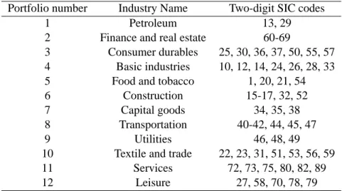
(15) Table 1. Portfolio definitions Portfolio number 1 2 3 4 5 6 7 8 9 10 11 12. Industry Name Petroleum Finance and real estate Consumer durables Basic industries Food and tobacco Construction Capital goods Transportation Utilities Textile and trade Services Leisure. Two-digit SIC codes 13, 29 60-69 25, 30, 36, 37, 50, 55, 57 10, 12, 14, 24, 26, 28, 33 1, 20, 21, 54 15-17, 32, 52 34, 35, 38 40-42, 44, 45, 47 46, 48, 49 22, 23, 31, 51, 53, 56, 59 72, 73, 75, 80, 82, 89 27, 58, 70, 78, 79. Note _ This table presents portfolios according to their number and sector as well as the SIC codes included in each portfolio using the same classification as Breeden, Gibbons and Litzenberger (1989).. p-values are obtained for the joint criterion (3.16).. 4. Empirical application Our empirical analysis focuses on the asset pricing model (2.2) with different distributional assumptions for stock market returns. We use nominal monthly returns over the period going from January 1926 to December 1995, obtained from the University of Chicago’s Center for Research in Security Prices (CRSP). As in Breeden et al. (1989), our data include 12 portfolios of New York Stock Exchange (NYSE) firms grouped by standard two-digit industrial classification (SIC). Table 1 provides a list of the different sectors used as well as the SIC codes included in the analysis.4 For each month the industry portfolios comprise those firms for which the return, price per common share and number of shares outstanding are recorded by CRSP. Furthermore, portfolios are value-weighted in each month. We proxy the market return with the value-weighted NYSE returns, also available from CRSP. The riskfree rate is proxied by the one-month Treasury Bill rate, also from CRSP. Our results are reported in Tables 2–3. We report, in addition to the asymptotic p-values [denoted pb∞ ] when available, three MC p-values: (i) the Gaussian based MC p-value [denoted pbg ], (ii) the Student t based MMC pvalue (maximized over all relevant degrees-of-freedom κ ≥ 2) [denoted pba ], and (ii) the Student t based CSMMC [denoted pbi ] (where the maximization is restricted to the degrees-of-freedom not rejected by a prior 2.5% goodness-of-fit tests); the associated confidence sets are reported in column 1 of Table 2. The results can be summarized as follows. 4. Note that as in Breeden et al. (1989), firms with SIC code 39 (Miscellaneous manufacturing industries) are excluded from the dataset for portfolio formation.. 10.

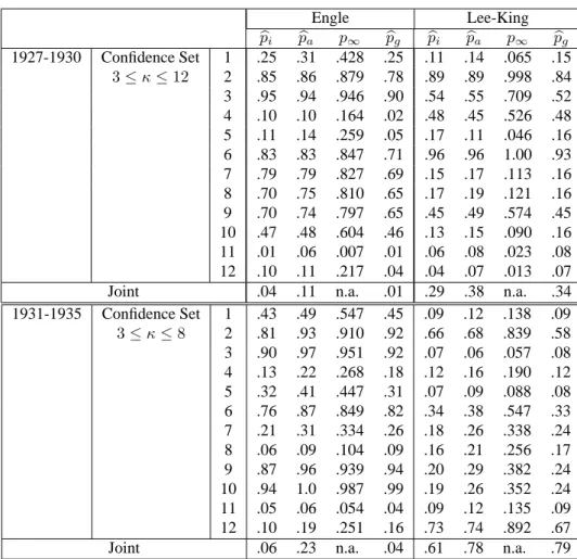
(16) Table 2. Univariate and Multivariate GARCH Tests. 1927-1930. 1931-1935. Confidence Set 3 ≤ κ ≤ 12. Joint Confidence Set 3≤κ≤8. Joint. 1 2 3 4 5 6 7 8 9 10 11 12 1 2 3 4 5 6 7 8 9 10 11 12. pbi .25 .85 .95 .10 .11 .83 .79 .70 .70 .47 .01 .10 .04 .43 .81 .90 .13 .32 .76 .21 .06 .87 .94 .05 .10 .06. Engle pba p∞ .31 .428 .86 .879 .94 .946 .10 .164 .14 .259 .83 .847 .79 .827 .75 .810 .74 .797 .48 .604 .06 .007 .11 .217 .11 n.a. .49 .547 .93 .910 .97 .951 .22 .268 .41 .447 .87 .849 .31 .334 .09 .104 .96 .939 1.0 .987 .06 .054 .19 .251 .23 n.a.. pbg .25 .78 .90 .02 .05 .71 .69 .65 .65 .46 .01 .04 .01 .45 .92 .92 .18 .31 .82 .26 .09 .94 .99 .04 .16 .04. pbi .11 .89 .54 .48 .17 .96 .15 .17 .45 .13 .06 .04 .29 .09 .66 .07 .12 .07 .34 .18 .16 .20 .19 .09 .73 .61. Lee-King pba p∞ .14 .065 .89 .998 .55 .709 .45 .526 .11 .046 .96 1.00 .17 .113 .19 .121 .49 .574 .15 .090 .08 .023 .07 .013 .38 n.a. .12 .138 .68 .839 .06 .057 .16 .190 .09 .088 .38 .547 .26 .338 .21 .256 .29 .382 .26 .352 .12 .135 .74 .892 .78 n.a.. pbg .15 .84 .52 .48 .16 .93 .16 .16 .45 .16 .08 .07 .34 .09 .58 .08 .12 .08 .33 .24 .17 .24 .24 .09 .67 .79. Note _ Numbers shown are MC p-values. p∞ refers to the test’s asymptotic p-value and pbg is the Gaussian based MC p-value. pbi is CSMMC p-value imposing student t(κ) errors (the method for constructing the underlying confidence set for the degrees-of-freedom κ is presented in Appendix A). pba is the MMC p-value overall degrees-of-freedom. The individual equation test statistic are: Engle’s T R2 and Lee-King’s statistic (3.5) defined in Section 3.2; the joint tests are defined in (3.6)-(3.7). n.a. means not available (because asymptotic critical values have not been derived).. 11.

(17) Table 2(b). Univariate and Multivariate GARCH Tests (continued). 1936–1940. Confidence Set 4 ≤ κ ≤ 29. 1941–1945. Joint Confidence Set κ≥5. 1946-1950. Joint Confidence Set 4 ≤ κ ≤ 31. Joint. 1 2 3 4 5 6 7 8 9 10 11 12 1 2 3 4 5 6 7 8 9 10 11 12 1 2 3 4 5 6 7 8 9 10 11 12. pbi .96 1.0 .48 .49 .48 .96 .18 .99 .15 .99 .12 .72 .16 .32 .13 .79 .11 .11 .44 .21 .39 .11 .52 1.0 .73 .90 .26 .66 .72 .05 .52 .95 .11 .61 .92 .15 .28 .57 .03. Engle pba p∞ .96 .937 1.0 .992 .52 .550 .62 .660 .52 .563 1.0 .986 .23 .281 1.0 1.00 .29 .317 1.0 .999 .26 .280 .85 .886 .33 n.a. .62 .656 .14 .203 .81 .851 .10 .128 .10 .137 .38 .433 .40 .457 .35 .416 .13 .171 .53 .561 1.0 .989 .65 .673 .90 n.a. .27 .320 .68 .729 .73 .789 .08 .086 .54 .598 .97 .963 .17 .255 .61 .679 .85 .864 .12 .161 .18 .282 .71 .766 .08 n.a.. 12. pbg .94 1.0 .43 .50 .50 1.0 .24 1.0 .17 1.0 .17 .79 .08 .55 .09 .78 .05 .05 .38 .15 .35 .06 .45 .99 .65 .87 .23 .64 .66 .03 .49 .91 .08 .60 .90 .09 .20 .57 .01. pbi .60 .87 .81 .24 .12 .29 .86 .64 .56 .74 .72 .20 .62 .98 .56 .54 .87 .12 .87 .16 .31 .21 .13 .31 .74 1.0 .16 .59 .63 .10 .52 .33 .88 .10 .55 .89 .81 .71 .81. Lee-King pba p∞ .66 .796 .87 .994 .81 .976 .31 .440 .17 .232 .37 .490 .89 .997 .66 .806 .55 .742 .73 .918 .74 .901 .25 .357 .67 n.a. .99 1.00 .54 .723 .57 .748 .85 .993 .11 .137 .85 .994 .15 .187 .31 .400 .21 .280 .13 .166 .31 .400 .80 .959 1.0 n.a. .14 .187 .64 .791 .65 .794 .10 .116 .28 .398 .40 .506 .72 .868 .10 .116 .67 .834 .92 .999 .76 .943 .75 .924 .83 n.a.. pbg .56 .84 .78 .24 .13 .33 .85 .60 .54 .68 .68 .21 .61 .95 .52 .49 .84 .10 .84 .12 .26 .14 .10 .26 .67 .99 .13 .53 .58 .08 .58 .29 .85 .08 .50 .84 .77 .67 .82.

(18) Table 2(c). Univariate and Multivariate GARCH Tests (continued). 1951-1956. Confidence Set 5 ≤ κ ≤ 34. 1956-1960. Joint Confidence Set κ≥5. 1961-1965. Joint Confidence Set κ≥7. Joint. 1 2 3 4 5 6 7 8 9 10 11 12 1 2 3 4 5 6 7 8 9 10 11 12 1 2 3 4 5 6 7 8 9 10 11 12. pbi 1.0 .34 .09 .99 .42 .25 .03 .29 .27 .96 1.0 .75 .22 1.0 .49 .53 .57 .36 .55 .44 .58 .72 .33 .21 .99 1.0 .64 .57 .99 .27 .88 .71 .88 .12 .30 .90 .15 .36 .47. Engle pba p∞ 1.0 .992 .31 .386 .09 .149 1.0 .990 .47 .510 .27 .350 .05 .024 .29 .367 .55 .597 .91 .900 1.0 .982 .71 .750 .32 n.a. 1.0 .993 .48 .547 .56 .626 .61 .640 .30 .396 .53 .633 .46 .531 .58 .667 .79 .807 .33 .424 .24 .320 .99 .977 1.0 n.a. .65 .693 .59 .639 .98 .973 .30 .350 .88 .869 .71 .768 .86 .884 .10 .147 .32 .374 .85 .895 .14 .185 .37 .425 .50 n.a.. 13. pbg 1.0 .32 .06 .99 .42 .23 .01 .26 .24 .92 .99 .70 .16 1.0 .42 .51 .52 .31 .49 .39 .53 .68 .28 .18 .98 1.0 .57 .47 .96 .25 .91 .65 .91 .07 .27 .92 .10 .28 .36. pbi .83 .64 .05 .08 .77 .11 .02 .11 .07 .77 .29 .52 .28 .66 .75 .86 .63 .39 .30 .03 .03 .18 .90 .08 .65 .67 1.0 .83 .83 .71 .83 .93 .68 .76 .84 .90 .49 1.0 .25. Lee-King pba p∞ .83 .987 .66 .810 .05 .054 .10 .108 .76 .933 .12 .128 .03 .017 .12 .127 .06 .058 .75 .904 .26 .356 .52 .677 .38 n.a. .70 .839 .77 .949 .87 .995 .66 .820 .51 .682 .29 .460 .03 .014 .03 .015 .18 .267 .91 .999 .10 .080 .70 .846 .67 n.a. 1.0 1.00 .84 .983 .84 .983 .73 .892 .82 .977 .94 1.00 .67 .828 .79 .963 .84 .986 .91 .999 .50 .684 1.0 1.00 .25 n.a.. pbg .77 .59 .05 .06 .69 .09 .02 .10 .06 .71 .26 .46 .37 .60 .71 .83 .57 .33 .25 .02 .02 .15 .89 .07 .59 .66 1.0 .78 .77 .66 .76 .89 .60 .73 .79 .87 .43 .97 .22.

(19) Table 2(d). Univariate and Multivariate GARCH Tests (continued). 1966-1970. Confidence Set κ≥5. 1971-1975. Joint Confidence Set 4 ≤ κ ≤ 28. 1976-1980. Joint Confidence Set 4 ≤ κ ≤ 17. Joint. 1 2 3 4 5 6 7 8 9 10 11 12 1 2 3 4 5 6 7 8 9 10 11 12 1 2 3 4 5 6 7 8 9 10 11 12. pbi .56 .83 .88 .51 .01 .45 .28 .30 .25 .04 .61 .05 .08 .06 .25 1.0 .42 .92 .97 .94 .50 .35 .12 1.0 .61 .36 .25 .27 .27 .15 .01 .04 .04 .82 .42 .15 .30 .18 .03. Engle pba p∞ .57 .619 .83 .853 .86 .870 .53 .586 .05 .005 .45 .491 .29 .339 .30 .355 .23 .277 .07 .056 .57 .606 .08 .092 .23 n.a. .09 .100 .25 .271 1.0 .999 .42 .464 .92 .915 .98 .954 .95 .940 .50 .563 .38 .416 .15 .184 .99 .964 .63 .673 .48 n.a. .25 .286 .33 .393 .27 .320 .16 .210 .02 .002 .07 .045 .09 .066 .85 .867 .42 .496 .15 .196 .36 .420 .22 .257 .11 n.a.. 14. pbg .49 .79 .85 .46 .01 .37 .23 .27 .20 .02 .51 .04 .05 .06 .21 1.0 .39 .89 .95 .91 .46 .33 .11 .99 .53 .32 .20 .26 .23 .14 .01 .01 .01 .82 .40 .13 .26 .17 .01. pbi .09 .84 .56 .09 .15 .95 .86 .91 .65 .51 .10 .68 .30 .10 .05 .28 .02 .14 .21 .21 .82 .62 .05 .37 .11 .26 .03 .93 .06 .05 01 .06 .01 .13 .13 .59 .90 .27 .03. Lee-King pba p∞ .09 .106 .83 .987 .57 .749 .09 .118 .15 .182 .96 1.00 .86 .995 .91 .999 .68 .827 .52 .701 .12 .129 .71 .850 .30 n.a. .11 .164 .05 .046 .28 .381 .02 .007 .16 .229 .22 .291 .22 .302 .83 .980 .63 .774 .05 .044 .40 .520 .11 .173 .28 n.a. .04 .014 .94 1.00 .06 .067 .05 .029 .01 .000 .07 .072 .01 .000 .16 .206 .16 .209 .59 .753 .90 .998 .31 .420 .03 n.a.. pbg .09 .79 .52 .09 .11 .90 .83 .86 .58 .47 .09 .62 .29 .10 .04 .22 .01 .11 .15 .18 .78 .58 .04 .34 .10 .24 .03 .89 .06 .03 .01 .06 .01 .12 .10 .52 .87 .23 .01.

(20) Table 2(e). Univariate and Multivariate GARCH Tests (continued). 1981-1985. Confidence Set 5 ≤ κ ≤ 33. 1986-1990. Joint Confidence Set 5 ≤ κ ≤ 41. 1991-1995. Joint Confidence Set κ ≥ 15. Joint. 1 2 3 4 5 6 7 8 9 10 11 12 1 2 3 4 5 6 7 8 9 10 11 12 1 2 3 4 5 6 7 8 9 10 11 12. pbi .70 .41 .80 .15 .11 .03 .01 .11 .62 .94 .65 .12 .08 .02 .44 .46 .50 .59 .86 .37 .62 .59 .14 .98 .06 .14 .71 .60 .76 .71 .99 .40 .36 .50 .79 .94 .52 .20 .86. Engle pba p∞ .72 .751 .41 .465 .78 .794 .16 .176 .08 .102 .06 .016 .02 .002 .11 .156 .68 .692 .94 .914 .61 .652 .18 .203 .21 n.a. .06 .021 .41 .557 .47 .598 .50 .654 .60 .727 .85 .879 .41 .558 .65 .760 .60 .719 .16 .277 .99 .981 .12 .152 .23 n.a. .71 .759 .61 .667 .75 .803 .68 .730 .99 .974 .44 .494 .39 .419 .53 .584 .81 .848 .94 .933 .53 .598 .20 .233 .88 n.a.. 15. pbg .67 .34 .76 .10 .07 .01 .01 .08 .61 .90 .63 .12 .06 .01 .35 .40 .45 .57 .82 .32 .59 .58 .12 .97 .04 .06 .64 .54 .73 .61 .98 .36 .27 .44 .76 .88 .48 .16 .76. pbi .96 .42 .99 .72 .19 .21 .57 .25 .08 .37 .95 .85 .12 .50 .12 .76 .31 .97 .58 .94 .88 .96 .72 .43 .81 .47 .31 .03 .96 .03 .74 .85 .02 .68 .09 .69 .17 .38 .31. Lee-King pba p∞ .96 1.00 .42 .577 1.0 1.00 .74 .902 .21 .262 .21 .270 .57 .728 .23 .332 .09 .081 .41 .552 .96 1.00 .87 .990 .14 n.a. .56 .673 .12 .091 .81 .930 .31 .355 .97 1.00 .64 .746 .94 .996 .88 .981 .96 .999 .79 .895 .43 .508 .87 .969 .47 n.a. .31 .370 .03 .020 .96 1.00 .03 .020 .75 .892 .85 .988 .02 .003 .68 .834 .09 .106 .70 .794 .17 .203 .38 .494 .31 n.a.. pbg .93 .39 .95 .65 .13 .16 .47 .20 .07 .34 .93 .84 .12 .50 .09 .67 .28 .96 .57 .89 .80 .95 .63 .38 .77 .47 .27 .02 .95 .02 .70 .80 .01 .64 .06 .60 .12 .34 .23.

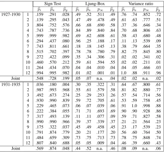
(21) Table 3. Univariate and Multivariate Predictability Tests. 1927-1930. Joint 1931-1935. Joint. 1 2 3 4 5 6 7 8 9 10 11 12 1 2 3 4 5 6 7 8 9 10 11 12. pbi .159 .139 .804 .743 .999 .294 .743 .515 .272 .460 .264 .994 .548 .036 .987 .492 .930 .229 .222 .317 .990 .175 .791 .484 .807 .569. Sign Test pba pbg .291 .028 .295 .043 .752 .576 .787 .736 .999 .982 .437 .080 .811 .661 .702 .397 .422 .099 .570 .212 .434 .070 .995 .982 .728 .199 .180 .004 .993 .968 .673 .274 .990 .839 .465 .073 .384 .055 .493 .139 .990 .966 .322 .037 .874 .779 .659 .309 .840 .688 .874 .048. pbi .49 .47 .66 .84 .69 .96 .18 .78 .35 .59 .04 .01 .05 .30 .55 .25 .59 .06 .71 .11 .39 .45 .20 .73 .05 .44. Ljung-Box pba p∞ .52 .511 .49 .478 .68 .690 .89 .840 .62 .608 .25 .188 .18 .145 .78 .780 .34 .306 .61 .594 .04 .010 .02 .001 .07 n.a. .35 .322 .61 .579 .29 .253 .72 .705 .07 .039 .71 .693 .11 .077 .37 .339 .49 .458 .21 .177 .75 .713 .05 .009 .52 n.a.. pbg .49 .49 .58 .84 .61 .17 .13 .79 .31 .55 .04 .01 .04 .31 .58 .26 .61 .06 .69 .09 .37 .45 .20 .73 .04 .46. pbi .76 .61 .37 .70 .58 .11 .38 .82 .02 .02 .04 1.0 .02 .64 .81 .57 .53 .91 .90 .59 .21 .23 .56 .78 .46 .08. Variance ratio pba p∞ .74 .852 .63 .777 .36 .646 .68 .806 .43 .680 .13 .539 .79 .664 .75 .845 .02 .341 .02 .211 .05 .466 .88 .911 .02 n.a. .67 .800 .82 .880 .54 .714 .59 .758 1.0 .998 .90 .928 .71 .827 .21 .564 .17 .539 .60 .764 .75 .848 .39 .660 .09 n.a.. pbg .72 .51 .34 .63 .48 .09 .35 .80 .02 .01 .03 .96 .02 .61 .77 .56 .45 .88 .86 .58 .23 .23 .50 .74 .43 .06. Note _ Numbers shown are MC p-values. p∞ refers to the test’s asymptotic p-value and pbg is the Gaussian based MC p-value. pbi is the CSMMC p-value imposing student t errors; the underlying confidence sets (see Appendix A) are reported in Table 2. pba is the MMC p-value overall degrees-of-freedom. The individual equation test statistics are: the sign test (3.15) defined in Section 3.4; the Variance ratios (3.9) and the LjungBox criteria (3.8); the joint tests are defined in (3.16)-(3.11)-(3.12).. 16.

(22) Table 3(b). Univariate and Multivariate Predictability Tests (continued). 1936-1940. Joint 1941-1945. Joint 1946-1950. Joint. 1 2 3 4 5 6 7 8 9 10 11 12 1 2 3 4 5 6 7 8 9 10 11 12 1 2 3 4 5 6 7 8 9 10 11 12. pbi .689 .982 .396 .538 .154 .120 .254 .239 .624 .817 .008 .844 .652 .684 .519 .270 .126 .283 .090 .094 .396 .784 .878 .288 .396 .303 .337 .540 .637 .693 .830 .160 .656 .022 .041 .257 .240 .511 .353. Sign Test pba pbg .798 .532 .997 .910 .693 .302 .670 .368 .451 .076 .391 .072 .477 .165 .486 .150 .791 .626 .838 .670 .169 .006 .892 .741 .722 .535 .772 .530 .731 .449 .585 .196 .377 .052 .619 .177 .380 .051 .337 .065 .530 .237 .920 .809 .944 .896 .580 .279 .683 .434 .604 .268 .556 .171 .737 .476 .785 .512 .782 .524 .876 .733 .433 .103 .803 .519 .174 .001 .215 .020 .458 .156 .487 .165 .661 .406 .581 .152. pbi .90 .87 .18 .93 .54 .66 .51 .11 .24 .90 .05 .79 .28 .90 .64 .95 .59 .92 .27 .08 .17 .35 .83 .64 .43 .79 .91 .09 .29 1.0 .57 .72 .18 .14 .43 .05 .95 1.0 .28. 17. Ljung-Box pba p∞ .90 .848 .85 .759 .16 .114 .97 .918 .57 .543 .70 .666 .54 .528 .11 .065 .32 .283 .93 .868 .06 .017 .85 .762 .28 n.a. .92 .854 .68 .653 .95 .892 .58 .563 .92 .862 .27 .255 .09 .049 .14 .088 .32 .311 .85 .801 .65 .583 .41 .381 .79 n.a. .91 .872 .08 .030 .35 .324 1.0 .989 .39 .316 .73 .687 .16 .104 .16 .106 .43 .374 .07 .024 .96 .920 1.0 .991 .30 n.a.. pbg .90 .83 .18 .94 .52 .69 .50 .09 .19 .91 .05 .77 .25 .90 .59 .95 .56 .90 .26 .07 .13 .30 .79 .59 .35 .74 .86 .07 .26 1.0 .53 .71 .16 .12 .41 .04 .90 .98 .30. pbi .99 .44 .59 .61 .86 .91 .86 .38 .19 .11 .05 .56 .92 .28 .35 .57 .70 .31 .21 .66 .40 .04 .61 .93 .10 .20 .76 .85 .02 .41 .17 .73 .55 .77 .32 .32 .97 .48 .08. Variance ratio pba p∞ 1.0 .997 .41 .679 .68 .828 .65 .809 .99 .974 .94 .947 .86 .927 .39 .674 .29 .612 .12 .512 .07 .436 .52 .745 .21 n.a. .28 .613 .39 .655 .58 .744 .10 .830 .33 .628 .23 .588 .72 .832 .36 .645 .05 .356 .65 .773 .99 .971 .12 .508 .21 n.a. .77 .842 .87 .890 .04 .345 .26 .593 .13 .517 .79 .851 .77 .840 .80 .874 .34 .324 .33 .627 .91 .930 .91 .925 .08 n.a.. pbg .96 .40 .52 .57 .84 .90 .85 .36 .17 .10 .05 .50 .92 .23 .31 .55 .64 .29 .19 .61 .35 .04 .60 .89 .07 .17 .71 .81 .02 .39 .14 .66 .54 .72 .28 .27 .93 .44 .05.

(23) Table 3(c). Univariate and Multivariate Predictability Tests (continued). 1951-1955. Joint 1956-1960. Joint 1961-1965. Joint. 1 2 3 4 5 6 7 8 9 10 11 12 1 2 3 4 5 6 7 8 9 10 11 12 1 2 3 4 5 6 7 8 9 10 11 12. pbi .298 .390 .840 .540 .274 .688 .094 .532 .161 .477 .383 .441 .313 .944 .294 .534 .787 .405 .277 .388 .445 .984 .616 .963 .959 .811 .641 .393 .774 .093 .460 .546 .506 .581 .964 .984 .034 .961 .654. Sign Test pba pbg .564 .155 .597 .320 .900 .781 .688 .365 .593 .192 .778 .519 .372 .054 .688 .376 .424 .101 .729 .393 .654 .301 .615 .287 .398 .159 .949 .929 .546 .209 .708 .450 .867 .732 .655 .261 .534 .217 .598 .274 .617 .287 .979 .953 .801 .539 .963 .924 .959 .978 .791 .697 .775 .517 .655 .337 .876 .724 .369 .044 .725 .397 .753 .494 .735 .400 .769 .581 .977 .857 .984 .939 .236 .006 .925 .899 .920 .556. pbi .58 .62 .41 .99 1.0 .01 .42 .18 .92 .70 .28 .68 .98 .60 .14 .88 .89 .04 .47 .40 .30 .53 .29 .69 .69 .91 .79 .64 .67 .87 .49 .58 .60 .88 .36 .44 .46 .54 .97. 18. Ljung-Box pba p∞ .59 .551 .69 .679 .41 .364 .98 .966 1.0 .997 .01 .000 .41 .367 .18 .139 1.0 .809 .67 .620 .26 .206 .74 .696 .98 n.a. .60 .568 .14 .547 .88 .837 .87 .835 .03 .006 .47 .453 .40 .388 .31 .272 .47 .448 .19 .168 .66 .627 .68 .631 .91 n.a. .79 .720 .64 .614 .67 .643 .84 .799 .47 .451 .59 .543 .58 .505 .90 .834 .35 .293 .41 .398 .47 .424 .57 .615 .97 n.a.. pbg .56 .58 .37 .97 .99 .01 .40 .13 .86 .67 .26 .66 .94 .59 .11 .85 .86 .04 .42 .36 .25 .46 .22 .67 .66 .85 .71 .60 .65 .85 .47 .54 .56 .87 .32 .39 .43 .52 .94. pbi .90 .03 .56 .79 .87 .25 .88 .25 1.0 .82 .39 .93 .17 .05 .03 .05 .34 .01 .32 .82 .56 .93 .02 .20 .71 .11 .86 .86 .10 .74 .06 .72 .12 .72 .13 .35 .06 .27 .68. Variance ratio pba p∞ .83 .877 .04 .318 .58 .761 .92 .934 1.0 .998 .24 .575 .88 .920 .26 .592 .85 .986 1.0 .995 .46 .705 .85 .896 .17 n.a. .05 .362 .02 .225 .05 .410 .34 .653 .01 .049 .31 .639 .83 .892 .58 .761 .89 .911 .02 .137 .21 .579 .65 .796 .11 n.a. .86 .911 .86 .912 .10 .492 .73 .830 .06 .403 .71 .821 .12 .505 .72 .829 .12 .518 .35 .645 .06 .350 .29 .615 .68 n.a.. pbg .86 .03 .55 .76 .85 .20 .85 .21 1.0 .78 .36 .89 .14 .04 .02 .05 .30 .01 .29 .75 .55 .92 .01 .15 .65 .09 .79 .78 .10 .67 .05 .67 .10 .67 .10 .28 .04 .24 .62.

(24) Table 3(d). Univariate and Multivariate Predictability Tests (continued). 1966-1970. Joint 1971-1975. Joint 1976-1980. Joint. 1 2 3 4 5 6 7 8 9 10 11 12 1 2 3 4 5 6 7 8 9 10 11 12 1 2 3 4 5 6 7 8 9 10 11 12. pbi .668 .680 .648 .951 .396 .375 .828 .437 .200 .379 .161 .312 .705 .827 .323 .661 .120 .126 .996 .196 .993 .453 .275 .967 .156 .191 .694 .865 .846 .689 .367 .986 .985 .643 .514 .131 .181 .807 .637. Sign Test pba pbg .789 .491 .784 .581 .841 .523 .937 .867 .632 .276 .645 .335 .828 .633 .598 .311 .492 .150 .589 .294 .402 .081 .562 .190 .728 .484 .841 .744 .562 .238 .810 .522 .377 .043 .333 .038 .998 .908 .420 .107 .993 .873 .588 .338 .524 .232 .967 .998 .448 .112 .597 .039 .792 .521 .891 .812 .884 .722 .764 .585 .601 .245 .986 .879 .999 .986 .839 .666 .663 .460 .346 .052 .448 .064 .885 .713 .743 .535. pbi .13 .33 .99 .75 .74 .26 .61 .86 .87 .87 .75 .83 .66 .16 .21 .72 .18 .23 .23 .46 .17 .84 .46 .87 .13 .40 .51 .94 .33 .86 .30 .14 .99 .08 .18 .30 1.0 .21 1.0. 19. Ljung-Box pba p∞ .16 .088 .33 .282 .99 .971 .75 .685 .74 .629 .28 .218 .60 .529 .87 .811 .87 .821 .87 .814 .75 .661 .84 .768 .66 n.a. .16 .124 .24 .191 .73 .679 .18 .152 .27 .220 .27 .225 .50 .436 .19 .158 .88 .828 .50 .450 .88 .822 .13 .096 .39 n.a. .56 .503 .93 .887 .31 .310 .86 .829 .32 .321 .14 .115 1.0 .973 .08 .040 .20 .177 .31 .312 1.0 .999 .94 .895 1.0 n.a.. pbg .10 .30 .97 .74 .68 .22 .56 .84 .84 .84 .74 .78 .55 .13 .18 .72 .17 .22 .23 .42 .17 .79 .42 .82 .08 .37 .48 .91 .26 .83 .26 .13 .98 .07 .17 .26 1.0 .90 .97. pbi 1.0 .37 .68 .59 .42 .20 .66 .76 .85 .88 .57 .49 .91 .55 .43 .97 .15 .16 .53 .52 .88 .88 .99 .84 .85 .28 .81 .46 .95 1.0 .65 .17 .71 .31 .35 .25 .99 .94 .24. Variance ratio pba p∞ 1.0 .998 .37 .660 .68 .806 .60 .773 .41 .684 .17 .568 .67 .800 .81 .868 .86 .903 .94 .931 .56 .754 .51 .720 .91 n.a. .55 .762 .42 .690 .96 .966 .16 .538 .16 .544 .53 .750 .52 .738 .89 .931 .87 .918 1.0 .997 .82 .894 .87 .903 .28 n.a. .78 .871 .48 .721 .98 .972 1.0 .991 .63 .794 .17 .541 .73 .833 .30 .620 .27 .609 .26 .604 1.0 .988 .96 .382 .24 n.a.. pbg .99 .31 .62 .54 .40 .16 .60 .72 .82 .86 .51 .45 .84 .49 .36 .92 .13 .14 .45 .45 .80 .78 .94 .74 .74 .24 .75 .43 .97 .99 .57 .16 .64 .26 .29 .24 .98 .04 .20.

(25) Table 3(e). Univariate and Multivariate Predictability Tests (continued). 1981-1985 –. Joint 1986-1990. Joint 1991-1995. Joint. 1 2 3 4 5 6 7 8 9 10 11 12 1 2 3 4 5 6 7 8 9 10 11 12 1 2 3 4 5 6 7 8 9 10 11 12. pbi .142 .191 .770 .987 .677 .342 .107 .984 .290 .388 .378 .511 .853 .917 .483 .546 .824 .489 .211 .623 .425 .781 .953 .799 .025 .734 .379 .279 .966 .811 .518 .081 .488 .442 .936 .260 .505 .376 .962. Sign Test pba pbg .405 .057 .501 .167 .882 .688 .990 .843 .783 .520 .660 .345 .344 .056 .984 .878 .567 .255 .602 .278 .662 .298 .690 .479 .922 .508 .964 .989 .732 .444 .721 .438 .914 .711 .693 .407 .559 .125 .808 .620 .647 .329 .889 .658 .953 .913 .857 .681 .251 .011 .734 .430 .653 .238 .540 .243 .966 .911 .919 .657 .748 .379 .369 .054 .675 .445 .690 .448 .993 .907 .563 .254 .716 .422 .611 .297 .969 .956. pbi .53 .22 .33 .91 .32 .76 .23 .49 .91 .14 .76 .26 .04 .57 .92 .80 .13 1.0 .62 .97 .28 .52 .37 .90 .99 .59 .20 .38 .57 .37 .46 1.0 .09 .98 .60 .24 .45 .33 .91. 20. Ljung-Box pba p∞ .53 .474 .22 .165 .33 .271 .90 .846 .35 .297 .75 .704 .23 .174 .53 .474 .94 .883 .15 .100 .77 .732 .24 .194 .04 n.a. .58 .542 .96 .901 .78 .747 .13 .080 1.0 .978 .64 .567 .96 .927 .28 .230 .53 .499 .34 .292 .91 .860 1.0 .973 .58 n.a. .20 .156 .38 .366 .55 .523 .37 .362 .46 .456 1.0 .990 .10 .039 .99 .945 .62 .581 .25 .200 .43 .423 .32 .313 .91 n.a.. pbg .47 .20 .30 .88 .30 .74 .20 .46 .88 .11 .76 .22 .02 .52 .93 .75 .09 .98 .54 .94 .25 .49 .34 .85 .98 .52 .16 .33 .55 .33 .39 1.0 .08 .97 .57 .23 .36 .30 .88. pbi .53 .35 .96 .52 .69 .93 .97 .29 .13 .65 .41 .53 .29 .62 .27 .06 .05 .92 .89 .51 .92 .72 .12 .32 .76 .48 .18 .56 .27 .18 .47 .51 .01 .95 .05 .96 .64 .98 .12. Variance ratio pba p∞ .55 .734 .35 628 .98 .970 .51 .703 .67 .801 .94 .940 .97 .959 .29 .602 .16 .535 .67 .798 .42 .668 .55 .732 .29 n.a. .63 .803 .30 .637 .07 .482 .05 .459 .93 .931 .87 .906 .50 .727 .94 .944 .63 .805 .12 .531 .39 .683 .77 .870 .48 n.a. .18 .554 .58 .773 .29 .620 .20 .576 .49 .729 .51 .742 .02 .065 .99 .979 .06 .331 .99 .973 .62 .800 .99 .978 .13 n.a.. pbg .47 .30 .92 .44 .62 .90 .91 .28 .12 .60 .35 .47 .24 .56 .22 .05 .03 .85 .81 .46 .87 .69 .06 .26 .72 .42 .15 .50 .24 .16 .47 .48 .01 .94 .04 .95 .59 .99 .08.

(26) 4.1. Overview of the results First, focusing on the univariate tests, we see that the asymptotic p-values may lead to underrejections, particularly in the case of the variance ratio test. In general, the MC p-values are lower than the asymptotic ones for GARCH and variance ratio tests. The converse seems to hold for the Ljung-Box tests; note that a small scale simulation study we performed in Dufour and Khalaf (2002a) suggested this test might over-reject in regression contexts. Second, our results illustrate the importance of considering multivariate tests. In many cases, whereas univariate tests detect significant serial correlations and/or GARCH effects, the joint tests do not detect significant departures form the null hypothesis of interest. Interestingly however, in some cases, multivariate tests are more powerful in rejecting the joint null. This occurs for example in the case of Engle’s test, in the 1946-50 sample, and for the Ljung-Box case, in the 1981-85 subsample. The smallest univariate p-value is 15%, yet the joint test p-value is only 4%. Recall that the univariate tests do not account for error covariances, which justifies such conflicts. Thirdly, the confidence set based MMC approach is useful here. Indeed, in many cases, if degrees-of-freedom which are not compatible with the data are allowed, GARCH effects may end up undetected. For example, refer to the joint Engle-type test in 1927-30, 1946-50, 1976-80; this also occurs more noticeably with univariate tests. Finally, we observe that almost invariably, the tests considered have led to conflicting decisions regarding the maintained hypothesis. For example, although in principle, Lee-King’s test is supposed to be superior to the Engle test (because it is designed to account for positivity of variance), we observe that in many cases, the Engle test is significant whereas its Lee-King counterpart is not. The same holds true for the Ljung-Box and Variance Ratio tests. Of course, a formal simulation study is required to assess the relative power of competing tests, yet the conflicts we observed with this well known data set is worth noting, particularly when using exact p-values, for conflicts in test decisions are often attributed to finite sample distortions. Overall, the multivariate diagnostics do not detect serious deviations from the i.i.d. assumption.5 The assumption of i.i.d. errors provides an acceptable working framework with this data set. This result supports the common practice of considering 5 years sub-groups to perform asset pricing tests (e.g. efficiency, spanning, etc.) tests which require i.i.d. errors.. 4.2.. Detailed discussion of the results. We next discuss the test results in details, across all subperiods. We use α to represent the level of the tests. • 1927-30 subperiod Gaussian-based Engle tests detect significant GARCH in equations 4, 5, 11 and 12 [for α ≥ 2% and 5%, 1% and 4% respectively]; the associated joint test is significant for α ≥ 1%. Note that the asymptotic Engle test is significant (p∞ = .007) only for equation 11. With Student t errors, the 5. Recall that in the case of the confidence set based MMC pbi , the cut-off level is 2.5% (if an overall level of 5% is desired) since 2.5% was used to construct the underlying confidence set.. 21.

(27) MC p-values for Engle’s tests exceed 10% for equations 4, 5 and 12; in the case of equation 11, GARCH-t effects are still significant for levels exceeding 3.5% (b pi = .01); the associated joint test remains marginally significant for α ≥ 6.5% (b pi = .04). Regarding Lee-King’s test, although the asymptotic p-values are less than 5% in the case of equations 5, 11 and 12, all MC p-values exceed 5% on univariate and joint levels. The MC variance ratio tests are significant at 5% in Gaussian and non-Gaussian cases, for equations 9, 10 and 11 and on a joint level. The MC Gaussian and non-Gaussian Ljung-Box tests are significant at 5% for equations 11 and 12; however, the associated joint test is significant for level exceeding 4% under Gaussian errors and levels exceeding 7% for non-Gaussian errors. Sign tests are significant (b pg = .028 and .043 respectively) only for equations 1 and 2. • 1931-35 subperiod Gaussian-based Engle tests detect significant GARCH in equations 11 and on a joint test basis [for α ≥ 4%]; the associated asymptotic test is not significant at 5% (p∞ = .054). With Student t errors, GARCH-t effects are still significant in this equation, for levels exceeding 6% (b pa = .06); the Student t joint test is marginally significant for α ≥ 8.5% (b pi = .06). Lee-King’s tests are not significant overall equations in this subperiod. While all variance ratio tests are not significant at conventional levels, the Ljung-Box MC test is significant at 5% in Gaussian and non-Gaussian context; with normal errors, the sign test is also significant at 5% for equation 9 and marginally (b pg = .055) for equation 6. However, the corresponding joint p-values exceed 44%. The sign test is significant for equation 1, for α ≥ .004 assuming normality and α ≥ 6.1% assuming t-errors; the associated joint test is significant (for α ≥ 4.8%) only under normality. • 1936-40 subperiod While all univariate p-values exceed 17%, the joint Gaussian-based Engle test has a p-value of 8%. Otherwise, no significant departure from the i.i.d. hypotheses are detected in this subperiod. Turning to Table 3, we see that the variance ratio, Ljung-Box and sign tests are all significant at 5% in the case of equation 11, under normality; in this case, with t-errors, the sign test remains significant (for α ≥ 3.3%) while the variance ratio and Ljung-Box are significant for α ≥ 7% and 6% respectively. All joint tests have p-values larger than 20%. • 1941-45 subperiod While all asymptotic univariate p-values exceed 20%, Gaussian-based Engle tests detect significant GARCH in equations 4 and 5 [for α ≥ 5%] and marginally for equation 9 [for α ≥ 6%]; however, the associated joint p-value is not significant (b pg = .87) and the same holds for the associated GARCH-t p-values which exceed 10%. Lee-King’s tests are not significant overall equations in this subperiod. MC p-values for the sign and Ljung-Box test all exceed 5%; Gaussian and t-based variance ratio tests are significant at 5% in equation 9 [for α ≥ 4%]. However, all associated joint p-values exceeds 21%. 22.

(28) • 1946-50 subperiod While all asymptotic univariate p-values exceed 8.6%, Gaussian-based Engle tests detect significant GARCH in equations 4 [for α ≥ 3%]; the associated joint p-value is highly significant (b pg = .01). In the case of GARCH-t p-values, the MC Engle tests detect significant GARCH for levels exceeding 7.5% (b pi = .05); the associated joint test is still significant for α ≥ 5.5%. Lee-King’s tests are also not significant in this subperiod. >From Table 3, we see that the MC variance ratios are significant at 5% in the case of equation 3, in normal and non-normal cases; on a joint basis, the normal based MC variance ratio test is significant at 5% whereas it t-based counterpart is significant at 8%. Regarding the MC Ljung-Box test, we see that it is significant in the case of equation 12, at α ≥ 4% under normality and α ≥ 7% under Student t errors; the test is however not significant on a joint level. Examining the sign test under normal errors, we find significant departures from the i.i.d. hypothesis in equations 8 and 9 (for α ≥ 0.1% and 2% respectively); under t-errors, the test remains significant in these equations (for α ≥ 5.7% and 6.6% respectively). The joint sign tests are not significant at conventional levels. • 1951-56 subperiod Gaussian-based Engle tests detect significant GARCH in equations 7 (b pg = .01) and marginally for equation 3 [for α ≥ 6%]; the associated joint test is however not significant, and the asymptotic Engle test is significant (p∞ = .024) only for equation 7. With Student t errors, the MC p-values for Engle’s tests exceed 9% for equations 3; in the case of equation 11, GARCH-t effects are still significant for levels exceeding 5% (b pa = .05); the associated joint test is not significant for levels. Regarding Lee-King’s test, we find find significant Gaussian and t-based p-values in both equations 3 and 7 (in equation 3, pbg = .05 and pba = .05; in equation 7, pbg = .02 and pba = .03). However, all joint Lee-King tests have p-values not smaller than 28%. With respect to tests predictability, the normal and non-normal variance ratio and Ljung-Box MC tests are significant at 5% for equations 2 and 6 respectively. However, all joint tests and all sign tests are not significant at usual levels. • 1956-60 subperiod While all Engle tests are not significant at conventional levels, Lee-King’s test detect significant GARCH in equations 7 and 8 with Gaussian and Student t errors (in both equations pbg = .02 and pba = .03). The asymptotic p-values also yield the same evidence. However, none of the joint p-values is significant (all exceed 60%). In this subperiod, the normal and non-normal variance ratio MC tests are significant at 5% for equations 1, 2, 3, 5 and 10. Despite such univariate evidence, the associated joint tests have p-values which exceed 9%. It is also worth noting that the asymptotic Variance Ratio test is not significant for equations 1, 2, 3 and 10. In the case of the Ljung-Box test, we find significant (at 5%) MC p-values under normal and non-normal errors only for equation 10; we note that the joint MC Ljung-Box p-values all exceed 85% and none of the sign tests is significant at usual levels. • 1961-65 subperiod 23.

(29) While all univariate p-values exceed 14%, the Gaussian-based Engle test has a p-value of 7% for equation 8. Otherwise, no significant departures from the i.i.d. hypotheses are detected in this subperiod. Turning to the Ljung-Box tests, we observe no significant p-values at standard levels. In contrast, the MC normal and non-normal sign test is significant (at 5%) for equation 11; the tests is significant at 5% given normal errors in equation 4, but the Student t p-values are not significant; the same holds true for the joint sign tests. Similarly, none of the Ljung-Box tests is significant. The variance ratio MC tests are significant, in equation 4 and 11, for α ≥ 5% and 4% respectively, under normality, and 6% under the Student t hypothesis; the associated joint p-values exceed 62%. • 1966-70 subperiod Gaussian-based Engle tests detect significant GARCH in equations 5, 10 and 12 [for α ≥ 1%, 2%, and 4% respectively]; the associated joint test is significant for α ≥ 5%. Note that the asymptotic Engle test is significant at 5% only for equation 5. With Student t errors, in the case of equation 5, GARCH effects are still significant for levels exceeding 3.5% (b pi = .01); for equations 10 and 12 GARCH-t effects are marginally significant for α ≥ 6.5% and 7.5% respectively; the associated joint test is not marginally significant (b pi = .08 and pba = .23). All Lee-King tests have p-values not smaller than 9%. Similarly, none of the predictability tests is significant at usual levels. • 1971-75 subperiod Gaussian-based Lee-King tests signal significant GARCH in equations 2, 4 and 10 [for α ≥ 4%, 1%, and 4% respectively]; the associated joint test is however not significant. With Student t errors, GARCH effects are still significant at 5% in all three cases. However, the joint p-values are not significant. Engle’s tests are not significant except for the Gaussian based case in equation 1, with a p-value of .06%. The serial correlation tests are all not significant at usual levels. The normal-errors based sign test is significant (at 5%) jointly and for equations 4 and 5. However, its t-based counterparts are not significant. • 1976-80 subperiod Gaussian and Student t based Lee-King tests are significant at 5% in equations 1, 4, 5 and 7; the associated joint tests all have p-values ≤ 3%. Engle’s tests provide the same evidence given Gaussian errors for equations 5, 6 and 7 and on joint basis. The Student t based Engle test for these equations is significant for levels exceeding 2%, 6.5% and 6.5% respectively; the joint Engle Student t based CSMMC p-value is 3%. Except for equation 12 under normality, the variance ratio tests are not significant. All MC Ljung-Box and sign tests exceed 5% in this subperiod. • 1981-85 subperiod. 24.

(30) While all Lee-King tests are not significant at conventional levels, Engle’s test is significant in equations 6 and 7 with Gaussian and Student t errors ( pbg = .01 in both equations; in equation 7, pba = .02 while in equation 6, Engle’s sup-MC test is significant for α ≥ 5.5%). However, joint p-values are not significant at 5%. In this subperiod, we note an interesting result regarding the Ljung-Box test: whereas all univariate tests are not significant, the joint MC normal and non-normal tests are significant at 5%. Recall that the joint tests are based on orthogonalized residuals, which corrects for cross-correlations. All other tests (univariate or multivariate) are not significant on a joint level. • 1986-90 subperiod While all Lee-King tests are not significant at conventional levels, Engle’s test is significant in equations 1 and 12 with Gaussian errors ( pbg = .01 and .04 respectively). However, there is evidence for GARCH errors only in equation 1 (b pa = .02). Furthermore, joint p-values are not significant at 5%. Similarly, none of the Ljung-Box tests is significant. The variance ratio MC tests are significant, in equation 3 and 4, for α ≥ 5% and 3% respectively, under normality, and for α ≥ 6% and 5% under the Student t hypothesis; the associated joint p-values exceed 52%. As for the sign test, we find significant MC normal and non-normal p-values (at 5%), in equation 12; however, this no longer holds on a joint test level. • 1991-95 subperiod In this subperiod, Engle tests are not significant jointly and individually Lee-King’s test is significant in equations 2 and 7 with Gaussian and Student t errors ( pbg = .02 and .01 respectively; in equation 7, pba = .02 while in equation 1, Lee-King’s sup-MC t-based test is significant for α ≥ 5.5%). However, all joint p-values exceed 23%. Turning to Table 3, we see that Sign tests and Ljung-Box tests are not significant jointly and individually The MC variance ratio test is significant in equations 7 and 9 with Gaussian and Student t errors ( pbg = .01 and .04 respectively; in equation 7, pba = .02 while in equation 9, the variance ratio sup-MC t-based test is significant for α ≥ 6%). However, all joint p-values exceed 8%.. 5. Conclusion Previous research typically assess MLR-based asset pricing statistical models using tests based on individual equations. Due to error cross-correlations, statistics from individual equations which are not independent, which raises simultaneous test problems. In this paper, we consider a diagnostic test procedure that accounts for cross-equation correlations exactly, in possibly non-normal contexts. We focus on departures from the i.i.d. errors hypothesis, on univariate and multivariate levels. Our univariate tests extend existing exact procedures by allowing for unspecified parameters in the error distributions. Our multivariate tests are invariant to MLR coefficients and error covariances; dependence on further unknown parameters in the error distribution is circumvented applying MC test techniques. We consider, tests for serial correlation, tests for multivariate GARCH and sign-type tests against general dependencies and asymmetries. The tests proposed are applied 25.

(31) to an asset pricing model with observable risk-free rates, using monthly returns on New York Stock Exchange (NYSE) portfolios over five-year subperiods from 1926-1995. Our tests reveal noticeable conflicts in the univariate versus multivariate procedures; this highlights the importance of formally controlling for contemporaneous correlation of disturbances.. 26.