Currency Total Return Swaps:
Valuation and Risk Factor Analysis
∗
Romain Cuchet
BRD — Groupe Société Générale
Pascal François
HEC Montréal and CIRPÉE
Georges Hübner
HEC Management School — University of Liège
Maastricht University
Gambit Financial Solutions
October 4, 2012
∗Corresponding author: Pascal François, HEC Montreal, Department of Finance, 3000 Cote-Ste-Catherine, H3T 2A7 Montreal, Canada. Mail to: [email protected]. We thank ING for kindly providing us with CTRS data, and Laurent Bodson for excellent research assistance. Financial supports from SSHRC (François) and Deloitte Luxemburg (Hübner) are gratefully acknowledged. All remaining errors are ours.
Currency Total Return Swaps: Valuation and Risk Factor Analysis
Abstract
Currency total return swaps (CTRS) are hybrid derivatives instruments that allow to simultaneously hedge against credit and currency risks. We develop a structural credit risk model to evaluate CTRS premia. Empirical test on a sample of 23,005 price observations from 59 underlying issuers yields an average percentage error of around 10%. This indicates that, beyond interest rate risk, firm-specific factors are major drivers of the variations in the valuation of these instruments. Regression analysis of residuals shows that exchange rate determinants account for up to 40% of model pricing errors — indicating that a currency risk premium affects the CTRS price significantly but only marginally, which confirms the prevalence of credit risk in the pricing of CTRS.
JEL Classification Numbers: G13, G15, G32.
1
Introduction
Financial innovation allows investors to trade on new products, thereby exchanging more accurate information on how to determine the equilibrium reward for exposure to various types of risks. Unlike bonds, whose observed price can be contaminated by supply and demand liquidity effects, the simple structure of symmetric financial derivatives such as futures and plain vanilla swaps provides the possibility to identify the fundamental drivers of their marked-to-market valuations. When the swap contract involves several very distinct sources of risk, the analysis can become more complex but remains valuable. In particular, it can shed light on the relative importance of the distinct sources of risk in the determination of market prices. For instance, with a contract that would involve interest rate and currency risk only, an adequate hedging strategy requires identifying the extent to which price fluctuations are only due to interest rate movements versus those that can be attributed to currency-specific risk factors.
In this paper, we study a recent kind of credit derivative involving cash flows de-nominated in different currencies. A Currency Total Return Swap (CTRS) is an over-the-counter credit derivative in which the buyer pays a floating return on the principal amount denominated in foreign currency, while the seller pays a floating return on the principal amount denominated in domestic currency. Entering into a CTRS contract therefore allows to simultaneously hedge against default and currency risks. Naturally, the credit risk of the underlying bond instrument drives a large proportion of price fluc-tuations of such a product, but it is necessary to identify its role through an adequate valuation scheme. For this purpose, our first aim is to derive the analytical pricing of the CTRS and identify the mechanisms through which it is impacted by credit and currency risks.
By construction, CTRS should be more exposed to foreign exchange risk than any other credit derivative as its cash flows directly involve different currencies. Our second and main objective is thus to investigate the extent to which the pricing of this type of credit derivative is affected by currency risk. This contributes to a relatively scarce empirical literature linking credit derivatives valuation with foreign exchange conditions. Skinner and Townend (2002) and Skinner and Diaz (2003) show that the 1998 Asian currency crisis only impacted the prices of credit default swaps (CDS) that were written on Asia-located entities. However, they reject the idea that currency risk might have increased the exposure to default risk. Rather, they attribute the increase in Asian CDS premia to a moral hazard problem based on underestimating the likelihood of issuer’s restructuring as a credit event. Carr and Wu (2007) work on Brazilian and Mexican evidence to document that sovereign credit default swaps are affected by currency risk. Zhang et al. (2010) establish Granger causality between some CDS indices and exchange rates with the U.S. dollar, but most of their results lose their significance when it comes to the exchange rate with the Euro.
The literature is therefore mixed as to whether credit derivatives are significantly im-pacted by currency risk, mostly because its impact on the plain vanilla CDS instrument cannot be precisely determined. With our approach, we can quantify very precisely the potential currency exposure by removing the whole impact of idiosyncratic credit risk from the CTRS price. Also, in order to avoid potential contamination from sovereign risk, our work focuses on developed economies as our sample CTRS are written on EMU and UK firms and involve U.S. dollar denominated cash flows. We can attribute most of the residual variation in CTRS prices to currency risk.
Our results shed new light on the pricing of credit derivatives in general, and CTRS in particular. The interest rate and credit risk components explains more than 80% of the variance of CTRS prices in our model Only a small residual fraction, lower
than 10%, results from currency-specific risk factors. As we get very little unexplained variance in prices, our empirical evidence tends to confirm that pure foreign exchange risk has little influence on the price of credit derivatives beyond the impact of sovereign default risk.
The rest of the paper is structured as follows. After a brief description of the CTRS contract in section 2, section 3 presents the valuation framework. Implementation of the model to the sample data is detailed in section 4. In section 5 we perform a risk factor analysis that allows to gauge the relative importance of credit and currency risks on CTRS premia. Section 6 concludes. Technical proofs are gathered in the appendix.
2
The CTRS contract
The CTRS is a special kind of Total Return Swap (TRS). In a TRS agreement, one party A makes payments on a periodic basis to a counterparty B. These payments are made on the return of an underlying asset (known as the reference asset). In return, counterparty B pays A a fixed return or a floating return (e.g. Libor) on the principal amount of the reference asset. In a standard floating rate TRS, the counterparty B pays a floating return based on Libor.
The CTRS can be seen as a floating rate TRS with the additional feature that the reference asset is a floating rate bond denominated in foreign currency. Let (resp. ) denote the domestic (resp. foreign) money market rate at time , and denote the exchange rate at time . Based on a face value of one monetary unit,
Party A commits to paying at time while counterparty B commits to paying
0
¡
−
¢
at time , where represents the premium for the CTRS
contract. The payoffs involved in a CTRS contract are represented in Figure 1.
The CTRS is designed to allow party A to simultaneously hedge against the default and currency risks of a foreign corporate bond. While party A swaps all payoffs from the foreign (defaultable) corporate bond to counterparty B, party A receives in turn the payments (in domestic currency) from a non-defaultable floating rate domestic bond.
For hedging purposes, payment frequency matches that of the underlying corporate bond. The standard contract maturity is 5 years. In case of default, party A stops its payment and pays the recovery value to B at maturity, while counterparty B’s commitments are unaffected.
Here is an example of a CTRS contract. The reference obligation is the senior unsecured bond issued by a European firm and denominated in euro. A U.S. investor wishes to hedge against the default and currency risks associated with this bond. A bank sells the U.S. investor a CTRS in which she commits to pay (in U.S. dollars) the returns from the U.S. Libor (less the CTRS premium). In return the U.S. investor transfers all payments received from the European bond to the bank.
3
Valuation framework
To evaluate the CTRS contract, one needs assumptions regarding the domestic and foreign term structure models, the exchange rate dynamics, and the default risk applying to the reference bond. These assumptions are detailed below.
3.1
Assumptions
Financial markets In the foreign and domestic economies, assets are continuously traded in arbitrage-free and complete markets. Following Amin and Jarrow (1991), the unique domestic risk-neutral probability measure Qis defined such that all discounted
risk-neutral probability measure Q is defined similarly for the foreign economy.
Foreign and domestic term structures The instantaneous domestic (foreign) risk-free interest rate follows an Ornstein-Uhlenbeck process under Q (Q), that is
= (− ) + ∈ { }
where represents the long-term equilibrium value of the process, is its mean
reversion speed and is the interest rate volatility. The process ( ≥ 0) is a
standard Wiener process under Q representing interest rate uncertainty. Subscript
denotes domestic () or foreign ( ) economy. Vasicek (1977) shows that the time- value for the riskless zero-coupon bond with one monetary unit due at time is given by
( ) = ( ) exp (−( ) ) ∈ { } with ( ) = exp à (( ) − ) ¡ 2− 22¢ 2 − 2 2( ) 4 ! ( ) = 1 − exp (− ) = −
Exchange rate dynamics Under Q the exchange rate 1 follows a lognormal
dif-fusion, i.e.
1
1
= ( − ) −
where is the constant volatility of the returns of the exchange rate, ( ≥ 0)
is the stochastic process representing the instantaneous domestic risk-free rate, and ( ≥ 0) is a standard Wiener process under Q accounting for the exchange risk.
Alternatively, under Qwe have
where ( ≥ 0) is a standard Wiener process under Q.
Assets of bond issuer The foreign firm capital structure is comprised of equity outstanding and debt. Without loss of generality, the face value of debt is normalized to 1, and the asset-to-debt ratio, denoted by , follows a lognormal diffusion process under Q
= +
where is the constant volatility of returns, and ( ≥ 0) is a standard Wiener
process under Q accounting for the business risk of the firm. We denote by the
correlation coefficient between ( ≥ 0) and ( ≥ 0).
Default rule The default boundary is denoted by and the default occurs at the
first hitting time defined as
= inf { ≤ : = }
where stands for the CTRS contract maturity. Following Briys and de Varenne (1997), the default boundary has an exponential shape and is expressed as a fraction of the risk-free (foreign) zero-coupon bond, that is,
= ( )
where 1 is a constant representing the critical value below which shareholders decide to leave the firm to creditors.
Recovery rule Debtholders recover only a fraction 1 of the assets upon default and the recovery rate is thus .
3.2
CTRS premium
Without any loss in generality, we consider a CTRS issued at a date 0 and maturing
at time . The fixing dates of the swap are denoted by , = 1 . The no-arbitrage
value for the CTRS is obtained by setting the value of the swap equal to zero at contract inception. To this end, we now explicitly compute the values of the two legs of the swap. One leg of the swap (what party A pays) simply consists of all cash flows stemming from the reference bond denominated in foreign currency. Let (0) denote the value
of this leg at time 0. It is given by
(0) = X =1 Q ∙ exp µ − Z 0 · ( +1) · 1 ¶¸ (1) +Q ∙ exp µ − Z 0 · 1 ¶¸ +Q ∙ exp µ − Z 0 · (0 ) · 1 ¶¸
In equation (1), ( +1) represents the foreign floating rate coupon and is equal to
the yield of the equivalent riskless bond, that is,
( +1) = − 1 +1− ln ( +1) = (+1− ) − ln (+1− ) +1−
Thus, the first term in equation (1) is the present value of all future foreign floating rate coupons conditional on no default. The second term in that equation is the present value of the principal repayment (normalized to 1) conditional on no default. The third term in that equation is the present value of the payment in case of default, which is a fraction of the equivalent riskless bond (0 ).
The following proposition provides with the no-arbitrage value for the reference obligation.
Proposition 1 The value of the reference obligation satisfies (0) = (0 ) ∙ Φ¡2¢− Φ ¡ −1 ¢¸ +(0 ) ∙ Φ¡−2¢+ Φ ¡ −1 ¢¸ + X =1 ( +1) (0 ) ∙ Φ¡ 2 ¢ −Φ¡− 1 ¢¸ with ( +1) = (+1− ) +1− " ¡ − ¢ −+ − 2 22 ¡ 1 − −¢2 # −ln (+1− ) +1− 1 = ln³ ( 0 ) ´ (0 ) + (0 ) 2 2 = 1 − (0 ) (0 ) = sZ 0 ³ 2 ( ) + 2 − 2( ) ´ ( ) = ( − )
and Φ () denotes the standard normal cumulative distribution function.
Proof: Detailed calculations for the three terms in equation (1) can be found, in the context of domestic bonds, in Briys and de Varenne (1997) and in François and Hübner (2004).
Expressed in foreign currency, the value of the other leg of the swap (what counter-party B pays), denoted by (0), is given by
(0) = X =1 Q ∙ exp µ − Z 0 ¶ ·0 · ( +1) ¸ (2) +Q ∙ exp µ − Z 0 ¶ ·0 ¸ − X =1 Q ∙ exp µ − Z 0 ¶ ·0 ¸
In equation (2), ( +1) represents the domestic floating rate coupon and its
The first term in equation (2) is the present value of all future domestic floating rate coupons converted into foreign currency (note that these payments are unconditional to the default event). The second term in equation (2) is the present value of the principal repayment converted into foreign currency. The third term in equation (2) is the present value of all CTRS premia , subtracted to what is party A is entitled to, converted
into foreign currency.
The no-arbitrage CTRS premium is therefore solution to
(0) = (0)
which leads to the following proposition.
Proposition 2 The premium of the CTRS denoted by satisfies
=
(0 ) − (0)
P
=1(0 )
where (0) is the value of the reference obligation given in Proposition 1 and
(0 ) = X =1 (0 ) ( +1) + (0 ) ( +1) = (+1− ) +1− ∙ (− ) −+ − 2 22 ¡ 1 − −¢2 ¸ −ln (+1− ) +1−
Proof: See appendix.
3.3
Sensitivity analysis
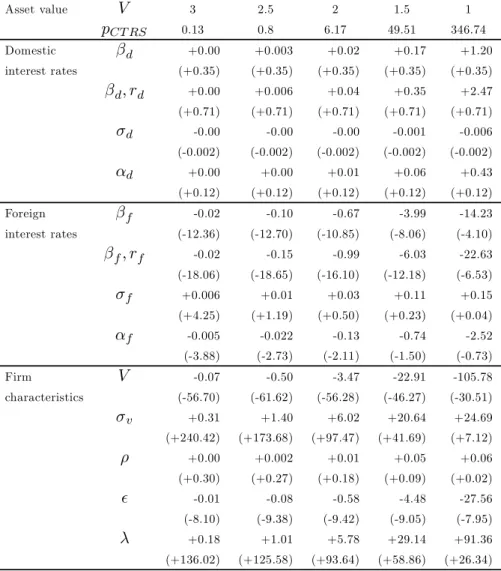
Table 1 reports the CTRS premium statics for various levels of leverage.
Insert Table 1 here
The CTRS premium (reported in basis points) decreases more than exponentially with the asset-to-debt ratio. By contract construction, it displays little sensitivity to
domestic interest rate parameters (which only interfere in the discounting of cash flows), but it is significantly affected by the foreign term structure level and slope (which interfere in the determination of cash flows). As expected, the greatest impacts on the CTRS premium stem from the underlying firm credit risk parameters, namely the asset-to-debt ratio and volatility as well as the default boundary. The largest sensitivities are observed for the latter two variables, but their importance varies across levels of leverage. When it is low (high asset value ), the distance to default is high and the key driver of the CTRS premium is asset volatility. As leverage increases, the default threshold becomes more prevalent, because the likelihood of default increases and affects both the probability of default and the expected recovery rate.
4
Model implementation
We apply the pricing results obtained in Propositions 1 and 2 to get the fitted prices of a sample of CTRS contracts. This will, in turn, enable us to identify the determinants of price variations related to default, interest rate, and currency risks.
4.1
Sample data
The dataset contains OTC quotations on CTRS issued by ING between September 1, 2005 and March 16, 2007. The reference obligations are written by European firms and are denominated in euro or in British pound while the bank payments are denominated in U.S. dollar. From the bank perspective, the U.S. dollar is the domestic currency and the foreign economy is the reference obligor’s.
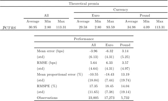
Insert Table 2 here
The database initially contains 125 firms, with 49,135 daily observations. We have restricted our sample to non-financial firms, incorporated in the Economic and Monetary
Union (EMU) or in the U.K., and listed on the stock market. The final sample contains 59 firms (listed in Table 2) and 23,005 daily observations.
Insert Table 3 here
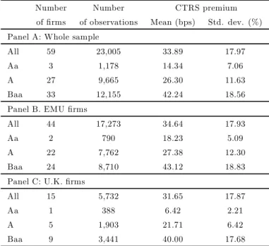
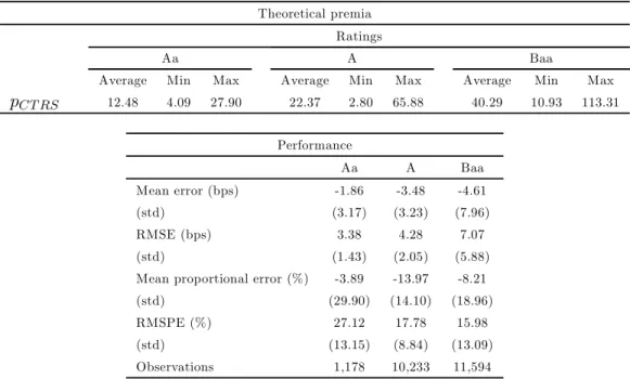
Table 3 reports the descriptive statistics for the CTRS premia and their breakdown across ratings and currencies. As expected, CTRS premia increase in level and become more volatile as the credit rating deteriorates. U.K. firms tend to have lower premia than the EMU ones, but the difference is not significant.
4.2
Estimation procedure
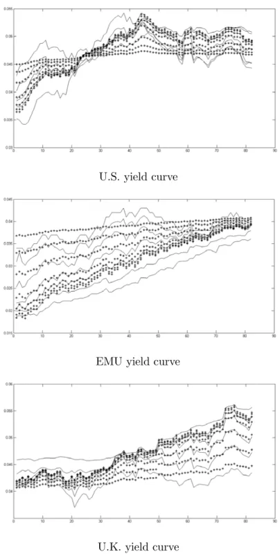
Interest rate parameters Parameters for the interest rate processes are estimated using the extended Kalman filter technique as in Duffee (1999) and Duan and Simonato (1999). Yield curves are collected on a weekly basis (Wednesday observation) with seven different maturities (3 and 6 months, 1, 2, 5, 10 and 20 years). Data for the U.S. rates are the Constant Maturity Treasury yields from the Federal Reserve of St-Louis. U.K. rates are obtained from the Bank of England, except for the 3 and 6 months maturity which are LIBOR rates. EMU rates are a composite index of French and German rates provided by Bloomberg. This index is well suited with our data since a majority of our sample firms (27 out of 44) are incorporated either in France or in Germany. Results for the Kalman filter estimations are reported in Table 4. Figure 2 provides with a visual inspection of the fit.
Insert Table 4 here Insert Figure 2 here
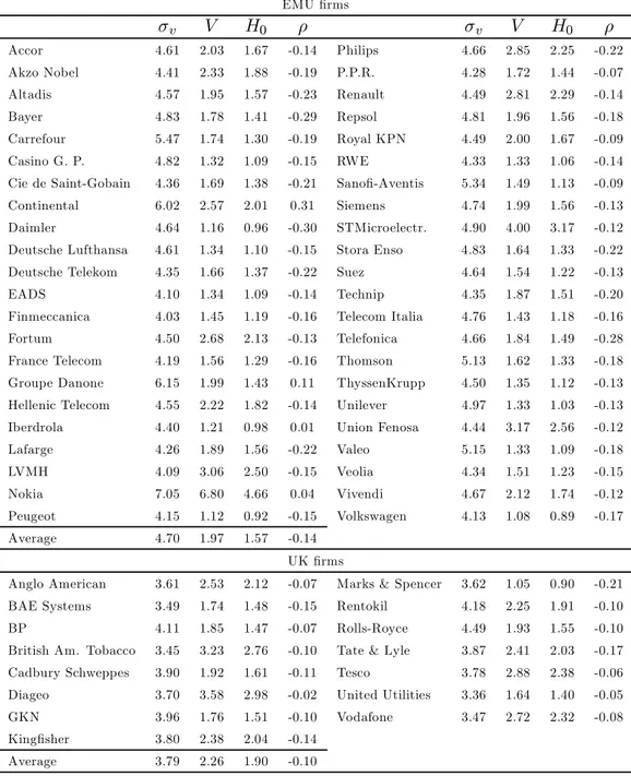
Firm characteristics Parameters and are obtained using a method which is
the theoretical CDS premium formula to infer a series of that is consistent with the observed quotations (5-year maturity CDS premia are obtained from Datastream). Then, is computed as the standard deviation of the returns on the inferred
asset-to-debt ratios and is the correlation coefficient between these returns and the risk-free interest rate. Using this series of and the computed and , parameter is calibrated
to minimize the squared errors of the theoretical model. This procedure is iterated until minimization of the squared errors. Results are reported in Table 5.
Insert Table 5 here
Because the model is using the asset-to-debt ratio (and not assets) as state variable, the estimated volatility levels are relatively lower (4.7% on average for EMU firms). On the other hand, the distance to default (defined as the ratio 0) is smaller (1.25 on
average for EMU firms). The asset-to-ratio is estimated at 1.97 on average for EMU firms, which corresponds to a leverage ratio of one third — in line with empirical studies on leverage (see e.g. Fan, Titman and Twite, 2010). As expected, correlation between asset-to-debt ratio and risk-free rate is slightly negative.
We use the following recovery rates obtained from Moody’s report (Hamilton and Varma, 2006) for the period under study: 57.04%, 49.54% and 45.48% for Aa, A and Baa ratings, respectively.
4.3
Model performance
In tables 6 and 7 we report the in-sample performance of the model. The pricing error is defined as the difference between the theoretical and observed premia. Since the model developed in section 2 essentially captures credit risk, its pricing performance provides a good indication about the relative importance of other sources of risk on CTRS premia.
Insert Table 7 here
Overall the model tends to slightly undervalue CTRS premia, with a mean error of almost 4 basis points (corresponding to a 11% proportional error). In absolute terms, the RMSE is 5.64% (i.e. 17.35% in proportion). Table 6 shows that the model undervalues CTRS labelled in euro and overvalues those labelled in British pound. This indicates that an exchange risk factor might be missing in the pricing of CTRS. Table 7 shows that the undervaluation slightly increases with the lower ratings, but not when measured by the RMSPE (i.e. the absolute error in proportion).
Insert Figure 3 here
Figure 3 plots the time series of theoretical and observed CTRS premia for a sub-sample of 6 firms (from all rating categories and both currencies). It visually confirms the undervaluation (resp. overvaluation) of CTRS written on EMU (resp. U.K.) firms. It also illustrates that the pricing error does not appear to be clustered in a particular subperiod. Similar patterns are found for the rest of sample firms (results available upon request).
The next section first investigates the behavior of the credit risk premium relative to the classical credit risk factors. Secondly, we study the residual in order to uncover the presence of an exchange and a liquidity components in the premia that is not captured by the pricing model.
5
Risk factor analysis
5.1
Credit risk premium
The aim of this subsection is to confirm that the model is indeed capturing a credit risk premium. According to structural models of credit risk, the credit risk premium should
be driven by three important factors: leverage, asset volatility and the risk-free rate. We closely follow the methodology of Ericsson et al. (2009) and perform the following regression on theoretical CTRS premia
( ) = + + + +
where ( ) is the theoretical CTRS premium of firm at time , a constant,
the financial leverage, the asset volatility and the risk-free rate.
Leverage is proxied by the ratio: book value of debt / (book value of debt + market value of equity). Balance sheet data are retrieved from Mergent Online. Asset volatility is proxied by the historical volatility of stock returns, computed from a 250 trading days rolling window. The risk-free rate is proxied by the one-year Libor rate.
Insert Table 8 here
Results are reported in table 8. Estimation is performed for each firm separately, and the reported coefficients are averages across firms coefficients.1 Following Collin-Dufresne et al. (2001), t-statistics are computed as follows
√
where is the mean coefficient for each explanatory variable, stands for the standard
deviation of these coefficients, and is the number of firms.
Overall the three variables have a high explanatory power on CTRS premia, with an adjusted R2ranging from 60% to 85% depending on rating category — figures comparable to the ones obtained in Ericsson et al. (2009). Financial leverage is globally significant at the 1% confidence level and has the expected sign. This result is mainly driven by lower
1Note that there are 300 more observations than in the dataset, which correspond to missing observed premia that have been interpolated in order to reach a balanced sample. Their exclusion does not alter the estimates.
rated (Baa) firms. Leverage is only significant for the EMU firms, but the t-statistic for the UK firms is at 1.64, extremely close to the 10% level. Volatility coefficients have the right sign but they are never significantly different from zero at any usual level. This is probably explained by the low variation in the volatility estimates used to compute the premia across the firms. The risk-free rate has the expected negative effect on the premia, and every coefficient is highly significant at the 1% level, whatever the currency or the rating. These regression results confirm that the theoretical model seems to adequately capture the credit risk component in the CTRS premia. The breakdown by credit rating appears to bring higher significance levels. This indicates that the main source of heterogeneity is likely to be found in credit qualities, which suggests that credit risk is the major driver of CTRS prices.
5.2
Analysis of pricing errors
The theoretical model implies that there is no currency risk component in the CTRS premium. In this section, we investigate the extent to which the CTRS premium ef-fectively contains a currency risk premium. The analysis is performed on the pricing error of the model. The rationale is that the model should have extracted all the credit component, leaving only liquidity effects and a random noise. To test this hypothesis, we regress the pricing error with most of the usual explanatory factors of the exchange rate. The factors are defined as the difference between the domestic and the foreign variables. In order to obtain comparable variables in the two economies, we standardize each variable before computing the difference. Consistently, the pricing error is also standardized. In the absence of a currency risk premium, none of these factors should be significant. The following regressors are used:
The exchange rate volatility If FX risk is priced, then the level of the risk premium should be related to exchange rate volatility. Nevertheless, since the volatility of the USD-GBP or the USD-EUR exchange rate is positively related to the volatility of the inverse exchange rate, the sign of the risk premium depends on the domestic currency of the purchaser of the contract. A negative sign would correspond to a dominance of U.K. or Eurozone purchasers, respectively, while a positive sign would be consistent with a larger share of the contracts held in majority by U.S. parties.
The nominal interest rates of the two economies The interest parity theory stipulates a relation between the interest rates differential and the exchange rate. Thus we expect them to have a possible effect on the residual. The data used are the 1-year Libor rates.
The price level and the inflation in the two economies The data used are the rate of variation of the monthly Harmonized Index of Consumer Prices from Eurostat for the EMU and U.K. economies and the Consumer Price Index from the Bureau of Labour Statistics for the U.S. economy.
Money supply Data are taken from Eurostat for the European economies and from the FED of St-Louis for the U.S. We use the monetary aggregate M2. Macroeco-nomic data have been linearly interpolated in order to have daily observations.
We also include GDP and the stock market index as control variables to account for the business cycle. GDP data are obtained from Eurostat and the FED websites. The stock market indices are the S&P 500, the Euronext 50 and the FTSE 100. As far as a liquidity variable is concerned, the bid-ask spread on the CTRS premia being unavailable, we include the bid-ask spread on CDS quotations. The underlying working assumption is that demand for CTRS is closely correlated with demand for CDS or, put
simply, that the most traded CDS should also be the most traded CTRS.
Insert Table 9 here
Table 9 reports the collinearity diagnosis. Correlation levels among explanatory variables are moderate, except maybe for GDP and the stock market index in the British economy. We compute the Variance Inflation Factor for each regressor and find that none of them exceeds 5 — which a commonly accepted criterion for rejecting multicollinearity issues in the regression analysis.
Regressions are performed for each firm separately, one including all the currency risk regressors, one adding the liquidity risk. We also run univariate regressions.
Insert Table 10 to 12 here
Tables 10 to 12 present the coefficients and their respective t-stats for the whole sample and for each currency zone. For the whole sample (Table 10), almost all the factors, with the exception of GDP, are significant at the 1% level, and have the expected sign. When combined together, only inflation and exchange rate volatility lose their significance. Currency risk factors account for 37% of total variance of the pricing error, and the residual pricing error, represented by the constant, does not appear to drift away from zero. Interestingly, the liquidity factor (as we proxy it using CDS bid-ask spread) does not contribute much to explaining pricing errors, as the adjusted R-square marginally increases by one or two percentage points as we include this variable.
Evidence presented in Tables 11 (EMU) and 12 (U.K.) confirm the contribution of each variable to the overall explanation of pricing errors. The significance level of the multiple regression reaches 34 % for EMU firms and 46% for U.K. firms. The major source of the difference between both sub-samples is the role of the exchange rate volatility factor. For EMU firms, it is negative in the single factor regression but
switches signs in the multiple one, and becomes weakly significant. We cannot infer any meaningful evidence about the currency risk premium from these results. For the U.K. sample however, there is a strong and robust negative relation between CTRS prices and FX volatility. Such a finding suggests that domestic U.K. investors are in majority long these contracts, inducing the negative sign of the corresponding currency risk premium. The small significance of the EMU premium could be explained by the nationality of the originator (ING) in the CTRS sample, which is primarily active in the EMU zone and thus mitigates the currency premium effect for these contracts, even though such an explanation warrants further investigation.
Overall, these results point to the presence of a currency risk premium, which ac-counts for a proportion that ranges from one third to one half of the variance in our model pricing errors. However, the pricing model proposed in Section 2, which reflects default and interest rate risk characteristics, makes an 11% proportional error on ob-served CTRS premia. Therefore, even though the explanatory power is satisfactory and confirms the influence of FX risk on the valuation of these contracts, we conclude that the contribution of a currency risk factor to the total premium is relatively marginal.
6
Conclusion
The interaction between default and currency risks is a topic that does not lend itself to an easy analysis. Through this paper, we have made a direct investigation of the relative influence of these two types of risks on the pricing behavior of derivatives that explicitly bear them, namely the CTRS. As a necessary step towards this end, we proposed a pricing approach of this hybrid contract based on the state-of-the-art literature on structural analysis of credit risk derivatives.
de-veloped for such instrument, has been tested on a proprietary and important sample of CTRS data. Our first conclusion is related to the quality of the pricing approach. Even though the asset volatility was indirectly estimated using stock market data, and despite the fact that the CTRS quotes can be contaminated by liquidity issues, the val-uation performance of the structural model is more than decent. Such a result, which holds independently of the factors affecting the time variations in the exchange rate risk premium, sheds light on the prevalence of default risk characteristics, mainly at the firm-specific level, over broad macroeconomic risk factors as drivers of a mixed credit-currency derivative.
Our empirical investigation of the determinants of the pricing error has confirmed our initial view. The factors affecting currency risk all have a significant influence on the residual variations of CTRS prices, but this influence is marginal compared to the default component. Thus, after considering a large set of potential drivers of CTRS price variations, we reach quite conclusive evidence that the explained part of the variance is very large when all factors are combined, but this type of contract clearly belongs to the class of credit risk instruments.
References
[1] Amin, K.I., and R.A. Jarrow, 1991, Pricing Foreign Currency Options Under Sto-chastic Interest Rates, Journal of International Money and Finance 10, 310—329.
[2] Briys, E., and F. de Varenne, 1997, Valuing Risky Fixed Rate Debt: An Extension, Journal of Financial and Quantitative Analysis 32, 239—248.
[3] Carr, P., and L. Wu, 2007, Theory and Evidence on the Dynamic Interactions between Sovereign Credit Default Swaps and Currency Options, Journal of Banking and Finance 31, 2383—2403.
[4] Collin-Dufresne, P., R. S. Goldstein, and S. Martin, 2001, The Determinants of Credit Spread Changes, Journal of Finance 56, 2177—2207.
[5] Duan, J.-C., and J.-G. Simonato, 1999, Estimating and Testing Exponential-Affine Term Structure Models by Kalman Filter, Review of Quantitative Finance and Accounting 13, 111—135.
[6] Duffee, G.R., 1999, Estimating the Price of Default Risk, Review of Financial Studies 12, 197—226.
[7] Ericsson, J., K. Jacobs, and R. Oviedo, 2009, The Determinants of Credit Default Swap Premia, Journal of Financial and Quantitative Analysis 44, 109—132.
[8] Fan, J., S. Titman, and G. Twite, 2010, An International Compari-son of Capital Structure and Debt Maturity Choices. Available on SSRN: http://ssrn.com/abstract=423483.
[9] François, P., and G. Hübner, 2004, Credit Derivatives with Multiple Debt Issues, Journal of Banking and Finance 28, 997—1021..
[10] Hamilton, D., and P. Varma, 2006, Default and Recovery Rates of Corporate Bond Issuers, 1920-2005, Moody’s Technical Report.
[11] Skinner, F., and A. Diaz, 2003, An Empirical Study of Credit Default Swaps, Journal of Fixed Income 13, 28—38.
[12] Skinner, F., and T. Townend, 2002, An Empirical Analysis of Credit Default Swaps, International Review of Financial Analysis 11, 297—309.
[13] Vasicek, O., 1977, An Equilibrium Characterization of the Term Structure, Journal of Financial Economics 5, 177—188.
[14] Vassalou, M., and Y. Xing, 2004, Default Risk in Equity Returns, Journal of Finance 59, 831—868.
[15] Zhang, G., J. Yau, and H.-G. Fung, 2010, Do Credit Default Swaps Predict Cur-rency Values? Applied Financial Economics 20, 439—458.
Appendix
Proof of proposition 2
The no-arbitrage condition (0) = (0) translates into
0 = − X =1 Q ∙ exp µ − Z 0 ¶ ·0 ¸ + X =1 Q ∙ exp µ − Z 0 ¶ ·0 · ( +1) ¸ +Q ∙ exp µ − Z 0 ¶ ·0 ¸ −(0)
Introducing the following change of probability measure Q Q = 0 exp µZ 0 (− ) ¶ = exp µ − Z 0 2 2 − Z 0 ¶ we get Q ∙ exp µ − Z 0 ¶ ·0 ¸ = Q ∙ exp µ − Z 0 ¶¸ = (0 ) Q ∙ exp µ − Z 0 ¶ ·0 · ( +1) ¸ = Q ∙ exp µ − Z 0 ¶ · ( +1) ¸
Using the domestic forward-neutral probability measure Q, we can write
Q ∙ exp µ − Z 0 ¶ · ( +1) ¸ = (0 ) Q[( +1)] Define ( +1) = Q[( +1)]. We obtain ( +1) = (+1− ) Q() − ln (+1− ) +1−
Under the forward neutral measure, the spot rate mean equals the current instantaneous forward rate. Hence
Q() = (− ) − + − 2 22 ¡ 1 − −¢2
Therefore = (0 ) − (0) P =1(0 ) with (0 ) = X =1 (0 ) ( +1) + (0 )
Figures
Figure 1: Currency Total Return Swap payoffs.
stands for the exchange rate at time , and is the CTRS premium. In case of
U.S. yield curve
EMU yield curve
U.K. yield curve
Figure 2: Observed and filtered yields for the U.S., European and British economies.
Figure 3: Time series of theoretical versus observed CTRS premia.
Theoretical premia are plotted with the dotted line and observed premia with the continuous line.
Tables
Asset value 3 2.5 2 1.5 1 0.13 0.8 6.17 49.51 346.74 Domestic +0.00 +0.003 +0.02 +0.17 +1.20 interest rates (+0.35) (+0.35) (+0.35) (+0.35) (+0.35) +0.00 +0.006 +0.04 +0.35 +2.47 (+0.71) (+0.71) (+0.71) (+0.71) (+0.71) -0.00 -0.00 -0.00 -0.001 -0.006 (-0.002) (-0.002) (-0.002) (-0.002) (-0.002) +0.00 +0.00 +0.01 +0.06 +0.43 (+0.12) (+0.12) (+0.12) (+0.12) (+0.12) Foreign -0.02 -0.10 -0.67 -3.99 -14.23 interest rates (-12.36) (-12.70) (-10.85) (-8.06) (-4.10) -0.02 -0.15 -0.99 -6.03 -22.63 (-18.06) (-18.65) (-16.10) (-12.18) (-6.53) +0.006 +0.01 +0.03 +0.11 +0.15 (+4.25) (+1.19) (+0.50) (+0.23) (+0.04) -0.005 -0.022 -0.13 -0.74 -2.52 (-3.88) (-2.73) (-2.11) (-1.50) (-0.73) Firm -0.07 -0.50 -3.47 -22.91 -105.78 characteristics (-56.70) (-61.62) (-56.28) (-46.27) (-30.51) +0.31 +1.40 +6.02 +20.64 +24.69 (+240.42) (+173.68) (+97.47) (+41.69) (+7.12) +0.00 +0.002 +0.01 +0.05 +0.06 (+0.30) (+0.27) (+0.18) (+0.09) (+0.02) -0.01 -0.08 -0.58 -4.48 -27.56 (-8.10) (-9.38) (-9.42) (-9.05) (-7.95) +0.18 +1.01 +5.78 +29.14 +91.36 (+136.02) (+125.58) (+93.64) (+58.86) (+26.34)Table 1: Comparative statics of the CTRS premium.
The numbers reported are the absolute changes in the CTRS premium after a 10% change in the parameter value. In parenthesis are reported the percentage variations of the premia. Base case parameters are: = 02, = 25, = 04, = 005, = 03, = 04,
EMU firms (44)
Aa Siemens Suez
A Akzo Nobel Bayer Carrefour Cie de St-Gobain Daimler
Deutsche Telekom EADS Finmeccanica Fortum France Telecom
Groupe Danone Hellenic Telecom Iberdrola Nokia Peugeot
RWE STMicroelectronics Sanofi-Aventis Telefonica Unilever
Veolia Environnement Volkswagen
Baa Accor Altadis Casino G. P. Continental Lufthansa
LVMH Lafarge Philips PPR Renault
Repsol Royal KPN Stora Enso Technip Telecom Italia
Thomson ThyssenKrupp Union Fenosa Valeo Vivendi
U.K. firms (15)
Aa British Petroleum
A Anglo American Diageo Tesco United Utilities Vodafone
Baa BAE Systems British Am. Tobacco Cadbury Schweppes GKN Kingfisher
Marks & Spencer Rentokil Rolls-Royce Tate & Lyle
Number Number CTRS premium of firms of observations Mean (bps) Std. dev. (%) Panel A: Whole sample
All 59 23,005 33.89 17.97
Aa 3 1,178 14.34 7.06
A 27 9,665 26.30 11.63
Baa 33 12,155 42.24 18.56
Panel B. EMU firms
All 44 17,273 34.64 17.93
Aa 2 790 18.23 5.09
A 22 7,762 27.38 12.30
Baa 24 8,710 43.12 18.83
Panel C: U.K. firms
All 15 5,732 31.65 17.87
Aa 1 388 6.42 2.21
A 5 1,903 21.71 6.42
Baa 9 3,441 40.00 17.68
Table 3: Descriptive statistics of CTRS premia.
The number of firms and observations do not add up to the total since four firms were downgraded from A to Baa during the sample period: Compagnie de Saint-Gobain, Daimler, Hellenic Telecom and Telefonica.
Panel A: Parameter estimates U.S. 0.38253 0.046382 0.004774 (0.044952) (0.000194) (0.000392) EMU 0.26646 0.041321 0.004721 (0.009625) (0.000185) (0.000397) U.K. 0.15273 0.040465 0.004666 (0.006185) (0.000176) (0.000378)
Panel B: Filter performance
U.S. EMU U.K.
Measurement Mean Measurement Mean Measurement Mean
error error RMSE error error RMSE error error RMSE
Maturity variance (bps) (bps) variance (bps) (bps) variance (bps) (bps)
3 months 14.81 -14.45 16.67 34.63 -32.24 32.52 20.21 15.3 15.57 6 months 5.20 3.26 4.61 17.68 -15.72 16.27 7.86 0.36 6.74 1 year 0.00 0.00 0.00 0.00 0.00 0.00 0.00 0.00 0.00 2 years 10.60 -6.68 9.27 8.74 3.29 6.54 5.93 -0.35 4.71 5 years 15.13 -7.83 14.54 15.14 -0.88 12.40 9.92 2.77 7.45 10 years 18.71 1.47 14.80 16.99 -2.07 14.14 12.98 3.48 10.04 20 years 20.65 25.95 26.56 20.32 -2.55 17.17 15.03 -4.5 13.2
Table 4: Kalman filter estimation of interest rates parameters.
The risk-neutral dynamics for the instantaneous spot rate are = (− ) +
. For each currency area, parameters are estimated using the extended Kalman filter
on the weekly yield curves observed between August 31, 2005 and March, 16 2007. In Panel A, standard deviations of the estimates are shown in parenthesis. In Panel B, the errors are defined as the difference between the actual and the fitted rates. Measurement error variance is multiplied by 104Mean errors and RMSE are reported in basis points.
EMU firms 0 0 Accor 4.61 2.03 1.67 -0.14 Philips 4.66 2.85 2.25 -0.22 Akzo Nobel 4.41 2.33 1.88 -0.19 P.P.R. 4.28 1.72 1.44 -0.07 Altadis 4.57 1.95 1.57 -0.23 Renault 4.49 2.81 2.29 -0.14 Bayer 4.83 1.78 1.41 -0.29 Repsol 4.81 1.96 1.56 -0.18 Carrefour 5.47 1.74 1.30 -0.19 Royal KPN 4.49 2.00 1.67 -0.09 Casino G. P. 4.82 1.32 1.09 -0.15 RWE 4.33 1.33 1.06 -0.14
Cie de Saint-Gobain 4.36 1.69 1.38 -0.21 Sanofi-Aventis 5.34 1.49 1.13 -0.09
Continental 6.02 2.57 2.01 0.31 Siemens 4.74 1.99 1.56 -0.13
Daimler 4.64 1.16 0.96 -0.30 STMicroelectr. 4.90 4.00 3.17 -0.12
Deutsche Lufthansa 4.61 1.34 1.10 -0.15 Stora Enso 4.83 1.64 1.33 -0.22
Deutsche Telekom 4.35 1.66 1.37 -0.22 Suez 4.64 1.54 1.22 -0.13
EADS 4.10 1.34 1.09 -0.14 Technip 4.35 1.87 1.51 -0.20
Finmeccanica 4.03 1.45 1.19 -0.16 Telecom Italia 4.76 1.43 1.18 -0.16
Fortum 4.50 2.68 2.13 -0.13 Telefonica 4.66 1.84 1.49 -0.28
France Telecom 4.19 1.56 1.29 -0.16 Thomson 5.13 1.62 1.33 -0.18
Groupe Danone 6.15 1.99 1.43 0.11 ThyssenKrupp 4.50 1.35 1.12 -0.13
Hellenic Telecom 4.55 2.22 1.82 -0.14 Unilever 4.97 1.33 1.03 -0.13
Iberdrola 4.40 1.21 0.98 0.01 Union Fenosa 4.44 3.17 2.56 -0.12
Lafarge 4.26 1.89 1.56 -0.22 Valeo 5.15 1.33 1.09 -0.18 LVMH 4.09 3.06 2.50 -0.15 Veolia 4.34 1.51 1.23 -0.15 Nokia 7.05 6.80 4.66 0.04 Vivendi 4.67 2.12 1.74 -0.12 Peugeot 4.15 1.12 0.92 -0.15 Volkswagen 4.13 1.08 0.89 -0.17 Average 4.70 1.97 1.57 -0.14 UK firms
Anglo American 3.61 2.53 2.12 -0.07 Marks & Spencer 3.62 1.05 0.90 -0.21
BAE Systems 3.49 1.74 1.48 -0.15 Rentokil 4.18 2.25 1.91 -0.10
BP 4.11 1.85 1.47 -0.07 Rolls-Royce 4.49 1.93 1.55 -0.10
British Am. Tobacco 3.45 3.23 2.76 -0.10 Tate & Lyle 3.87 2.41 2.03 -0.17
Cadbury Schweppes 3.90 1.92 1.61 -0.11 Tesco 3.78 2.88 2.38 -0.06
Diageo 3.70 3.58 2.98 -0.02 United Utilities 3.36 1.64 1.40 -0.05
GKN 3.96 1.76 1.51 -0.10 Vodafone 3.47 2.72 2.32 -0.08
Kingfisher 3.80 2.38 2.04 -0.14
Average 3.79 2.26 1.90 -0.10
Table 5: Firms parameters estimates.
The dynamics of the firm asset-to-debt ratio are given by= +.
Volatil-ity is reported in percentage. 0 stands for the initial level of the default boundary and is
defined as0= (0 )with = 5years. Coefficientis the correlation between the firm
assets and the risk-free rate. Parameters have been estimated using the iterative procedure on CDS data between 09/01/2005 and 03/16/2007.
Theoretical premia
Currency
All Euro Pound
Average Min Max Average Min Max Average Min Max
30.95 2.80 113.31 29.58 2.80 93.59 34.98 4.09 113.31
Performance
All Euro Pound
Mean error (bps) -3.96 -6.32 3.14
(std) (6.13) (4.31) (5.25)
RMSE (bps) 5.64 6.33 3.57
(std) (4.64) (4.31) (4.97)
Mean proportional error (%) -10.55 -18.43 13.19
(std) (18.04) (7.44) (19.74)
RMSPE (%) 17.35 18.45 14.04
(std) (11.65) (7.38) (19.14)
Observations 23,005 17,273 5,732
Table 6: Model performance: Overall and per currency.
Error is defined as the difference between the theoretical and observed premia. RMSE measures the pricing error in absolute terms. Proportional error is mean error divided by observed premium. Root Mean Squared Proportional Error (RMSPE) measures the proportional error in absolute terms.
Theoretical premia Ratings
Aa A Baa
Average Min Max Average Min Max Average Min Max
12.48 4.09 27.90 22.37 2.80 65.88 40.29 10.93 113.31 Performance Aa A Baa Mean error (bps) -1.86 -3.48 -4.61 (std) (3.17) (3.23) (7.96) RMSE (bps) 3.38 4.28 7.07 (std) (1.43) (2.05) (5.88)
Mean proportional error (%) -3.89 -13.97 -8.21
(std) (29.90) (14.10) (18.96)
RMSPE (%) 27.12 17.78 15.98
(std) (13.15) (8.84) (13.09)
Observations 1,178 10,233 11,594
Table 7: Model performance per ratings.
Error is defined as the difference between the theoretical and observed premia. RMSE measures the pricing error in absolute terms. Proportional error is mean error divided by observed premium. Root Mean Squared Proportional Error (RMSPE) measures the proportional error in absolute terms.
Total Per currency Per rating
Euro Pound Aa A Baa
Constant 16.45 -23.39** 36.18*** 8.72 39.13** 18.26 30.16** 2.46 t-stats (1.45) (-2.25) (12.03) (0.64) (2.07) (1.55) (2.21) (0.12) Leverage 44.57*** 88.27*** 40.18** 57.42 13.93 13.27 78.66*** (2.77) (5.09) (2.21) (1.64) (0.75) (0.75) (2.72) Volatility 14.40 3.76 2.61 48.98 4.52 0.72 30.43 (1.11) (0.29) (0.91) (0.97) (0.76) (0.24) (1.12) LIBOR -4.66*** -4.35*** -5.59*** -3.80*** -5.96*** -4.05*** (-6.39) (-5.91) (-2.90) (-4.15) (-6.68) (-3.26) R2 0.64 0.37 0.29 0.61 0.44 0.85 0.66 0.60 # obs. 23,305 23,305 23,305 17,380 5,925 1,185 10,665 11,455
Table 8: Credit factors regression results.
Reported coefficients are the average coefficients of the regression performed on each firm. Corresponding t-stats are in parenthesis.
EMU
Panel A: Correlation matrix
Libor Inflation Money supply Prices GDP Index FX vol Liquidity
1 -0.10 1 -0.32 0.24 1 -0.22 0.01 0.23 1 0.15 -0.28 0.33 0.17 1 -0.50 0.26 0.14 -0.09 -0.38 1 0.34 -0.02 -0.56 -0.33 -0.15 -0.25 1 -0.24 -0.01 0.08 0.12 -0.09 0.16 0.10 1
Panel B: Variance Inflation Factors
1.70 1.37 2.13 1.31 1.66 1.79 2.00 1.35
U.K.
Panel A: Correlation matrix
Libor Inflation Money supply Prices GDP Index FX vol Liquidity
1 -0.25 1 -0.07 0.18 1 0.33 -0.13 0.37 1 0.67 -0.17 -0.36 0.36 1 -0.70 0.14 -0.08 -0.48 -0.60 1 0.57 -0.02 -0.35 0.26 0.77 -0.57 1 -0.09 -0.07 0.05 -0.06 -0.10 0.16 -0.31 1
Panel B: Variance Inflation Factors
2.68 1.23 2.21 1.91 4.15 2.63 3.31 1.27
Table 9: Collinearity diagnosis.
In panel A, Table 9 reports the correlation matrix among explanatory variables. In panel B, Table 9 reports the Variance Inflation Factor (VIF) associated to each of the explanatory variables.
Constant 0.00 -0.18*** 0.00*** 0.00 0.00** 0.00 0.00 0.00* -0.00 -0.47*** (0.94) (-3.10) (2.71) (0.63) (2.07) (0.54) (1.36) (1.83) (-0.25) (-4.84) Libor -0.37*** -0.36*** -0.44*** (-7.31) (-7.62) (-7.86) Inflation 0.01 0.01 0.03*** (0.48) (0.96) (2.37) Money supply 0.79*** 0.70*** 1.37*** (3.41) (3.14) (6.91) Prices 0.18** 0.17** 0.34*** (2.11) (2.07) (4.57) GDP 1.05*** 1.02*** 0.23 (4.83) (4.87) (1.50) Index 0.20*** 0.17*** 0.45*** (3.11) (2.79) (5.49) FX volatility -0.12 -0.11 -0.16*** (-1.54) (-1.58) (-4.43) Liquidity 0.06*** 0.16*** (3.45) (4.90) R2 0.37 0.38 0.11 0.01 0.04 0.05 0.05 0.05 0.10 0.07
Table 10: Pricing errors regression — Whole sample.
Dependent variable is the standardized pricing error on the CTRS model. Reported coef-ficients are the average coefficients of regressions performed on each firm. The corresponding t-stats are reported in parenthesis.
Constant 0.00*** -0.13* 0.00*** -0.00 0.00*** 0.00*** 0.00 0.00* 0.00 -0.34*** (2.59) (-1.85) (2.85) (-0.85) (2.29) (3.56) (0.67) (1.87) (0.36) (-2.90) Libor -0.44*** -0.43*** -0.56*** (-7.34) (-7.66) (-8.82) Inflation -0.00 0.00 0.04*** (-0.10) (0.29) (3.36) Money Supply 0.82*** 0.71*** 1.76*** (2.65) (2.41) (7.78) Prices 0.49*** 0.47*** 0.60*** (8.24) (8.28) (11.82) GDP 0.52*** 0.53*** 0.33* (2.79) (2.87) (1.67) Index 0.34*** 0.31*** 0.52*** (5.09) (4.94) (5.19) FX volatility 0.11* 0.09 -0.11*** (1.66) (1.61) (-2.36) Liquidity 0.05** 0.12*** (2.17) (3.06) R2 0.34 0.35 0.12 0.01 0.05 0.06 0.05 0.05 0.10 0.06
Table 11: Pricing errors regression — EMU firms.
Dependent variable is the standardized pricing error on the CTRS model. Reported coef-ficients are the average coefficients of regressions performed on each firm. The corresponding t-stats are reported in parenthesis.
Constant 0.00 -0.32*** 0.00 0.00 0.00 -0.00 0.00 0.00 -0.00 -0.88*** (0.43) (-3.71) (1.58) (0.88) (1.15) (-0.97) (1.33) (1.49) (-0.44) (-6.22) Libor -0.14*** -0.14*** -0.10 (-2.53) (-2.65) (-1.53) Inflation 0.03 0.03* -0.01 (1.45) (1.66) (-0.23) Money Supply 0.71*** 0.67*** 0.21 (4.86) (4.47) (0.97) Prices -0.71*** -0.68*** -0.43*** (-5.54) (-5.50) (-4.50) GDP 2.62*** 2.47*** -0.04 (5.48) (5.37) (-0.20) Index -0.22*** -0.25*** 0.26** (-2.40) (-2.71) (1.98) FX volatility -0.77*** -0.71*** -0.32*** (-6.07) (-5.85) (-12.44) Liquidity 0.11*** -0.30*** (3.57) (5.30) R2 0.46 0.48 0.06 0.01 0.01 0.03 0.04 0.04 0.11 0.10
Table 12: Pricing errors regression — U.K. firms.
Dependent variable is the standardized pricing error on the CTRS model. Reported coef-ficients are the average coefficients of regressions performed on each firm. The corresponding t-stats are reported in parenthesis.