Implementation, Identification and Control of an Efficient Electric Actuator for Humanoid Robots

HAL Id: hal-01494676

https://hal.archives-ouvertes.fr/hal-01494676v3

Submitted on 25 May 2018

HAL is a multi-disciplinary open access

archive for the deposit and dissemination of

sci-entific research documents, whether they are

pub-lished or not. The documents may come from

teaching and research institutions in France or

abroad, or from public or private research centers.

L’archive ouverte pluridisciplinaire HAL, est

destinée au dépôt et à la diffusion de documents

scientifiques de niveau recherche, publiés ou non,

émanant des établissements d’enseignement et de

recherche français ou étrangers, des laboratoires

publics ou privés.

Implementation, Identification and Control of an

Efficient Electric Actuator for Humanoid Robots

Florent Forget, Kevin Giraud-Esclasse, Rodolphe Gelin, Nicolas Mansard,

Olivier Stasse

To cite this version:

Florent Forget, Kevin Giraud-Esclasse, Rodolphe Gelin, Nicolas Mansard, Olivier Stasse.

Implementa-tion, Identification and Control of an Efficient Electric Actuator for Humanoid Robots. International

Conference on Informatics in Control, Automation and Robotics (ICINCO 2018), Jul 2018, Porto,

Portugal. �hal-01494676v3�

Implementation, Identification and Control

of an Efficient Electric Actuator for Humanoid Robots

Florent Forget

and Kevin Giraud-Esclasse

and Rodolphe Gelin

and Nicolas Mansard

and Olivier

Stasse

1_{CNRS - LAAS, Toulouse, France, firstname.lastname@laas.fr}

2_{SoftBank Robotics Europe, Paris, France, gelin@aldebaran-robotics.com}

Keywords: Actuation, Humanoids

Abstract: Autonomous robots such as legged robots and mobile manipulators imply new challenges in the design and

the control of their actuators. In particular, it is desirable that the actuators are back-drivable, efficient (low friction) and compact. In this paper, we report the complete implementation of an advanced actuator based on screw, nut and cable. This actuator has been chosen for the humanoid robot Romeo. A similar model of the actuator has been used to control the humanoid robot Valkyrie. We expose the design of this actuator and present its Lagrangian model. The actuator being flexible, we propose a two-layer optimal control solver based on Differential Dynamical Programming. The actuator design, model identification and control is validated on a full actuator mounted in a work bench. The results show that this type of actuation is very suitable for legged robots and is a good candidate to replace strain wave gears.

1

INTRODUCTION

Mobile robots, such as legged robots and hu-manoid robots, imply new challenges in the design of their actuation system. In this context, it is very im-portant that the robot is able to feel the force that it ex-erts on its environment. At the same time, the actuator must be light-weight and compact. Direct-drive actu-ation is then not an option. On many electric-powered humanoid robot, strain wave gears (e.g. Harmonic Drive gear) are used for their compactness. How-ever, if back-drivable, strain wave gears have a poor transparency, i.e. the torque exerted at the joint level (output) is poorly correlated to the torque at the mo-tor level (input), and the output mo-torque is difficult to estimate from the motor current. If an accurate joint-torque estimation is needed, a joint joint-torque sensor must be added to the robot design, which increases the to-tal design cost and the actuation flexibility. Moreover, strain-wave gears are sensitive to impacts, which tend to damage the gear. Their maximum torques are also limited, in particular when impacts have to be ex-pected. For the design of full-size humanoid robots (i.e. size similar to Shaft, NASA Valkyrie, PAL Ta-los), strain-wave gears are clearly one of the main limiting factor of the design. On the other hand, most of alternative gears are either not compact enough, or with insufficient reduction ratio.

The design of such kind of actuators is a widely

Figure 1: The leg of the robot Romeo are designed based on a screw-nut-cable actuator, which are shock-proof and low-friction, but induce a flexibility due to the cable.

studied subject. Different technologies are used to ad-dress these problems. Electric-based actuation is very desirable because it is simple to implement, hence also more reliable for a given integration effort. A first step is to adapt electric motors to humanoid robotics needs as it is done in (Wensing et al., 2017) for quadruped robot. By increasing the motor diame-ter, the nominal speed is lowered while the nominal

torque is improved, allowing to reduce the reduction ratio and so having a more backdrivable system. An-other route is to improve the design of the gear box, as done in (Englsberger et al., 2014) where authors chose to improve strain-wave gears technology to build a torque-controlled robot. However, despite the improvement, strain-wave gear implies many draw-backs: insufficient torque limit, sensitivity to impact, lack of efficiency and of transparency. Adding a pas-sive element at the gear output releases a part of the limitations: it protects the gear from impact. It also makes a part of the actuation transparent, while an en-coder may be used to directly (after calibration) mea-sure the torque applied on the joint side. However, the passive element makes the actuation more difficult to control and intrinsically lowers the possible con-trol bandwidth, which is not desirable for achieving fast-dynamics movements. Variable-stiffness actua-tors as in (Wolf and Hirzinger, 2008) makes it pos-sible to dynamically stiffen the robot when high dy-namics is needed, but then boiling down to the same limits as rigid electric actuation. On a quite different route, hydraulic technology is promising to conceive robotics actuators allowing good power to weight ra-tio and shock absorpra-tion (Semini et al., 2011; Alfayad et al., 2011), although the implementation of the com-plete robot becomes more challenging.

In this paper, we present the complete implemen-tation (design, modeling, identification and control) of a screw-nut-cable compact actuator based on (Gar-rec, 2010). This actuator has been used to design the legs of the humanoid robot Romeo (see Fig. 1). A similar model of the actuator has been used to control the humanoid robot NASA R5 (Valkyrie) (Mehling, 2015), although the control strategy built upon it is different from ours. In the context of the new NASA challenge with this humanoid robot, the work pre-sented in this paper is very relevant.

The actuator offers reduction ratio up to 150 while keeping compact design. It has a high tolerance to shocks and impacts and offers a high transparency, making it reliable to estimate output torques from motor currents. It also induces flexibility coming from the cable connecting the screw to the joint out-put. Adding elasticity into the actuation smoothes the contact with the environment, which prevent re-bound and in certain case sliding effects (Lee et al., 2016). The flexible element in this particular gear can also be exploited to directly measuring the output torques, by equipping it with sensor able to measure the spring deflection (e.g. angle encoders attached to each side of elasticity). We show that measures of torques/forces can be obtained for quasi-null addi-tional cost. The flexible element behaves like a

series-(4) Geared-wheel, (5) Ball-screw Turn-buckle (12) Joint (11) (2) Pinion, (3) Toothed-belt (1) Motor Joint Encoder (14) Cable (9) Top end stop (10) Ball crimped on the cable Ball sleeve (7) Flexible coupling (6) Screw (5) (hollow-screw) (8) Fitted shaft Nut and Geared-wheel (4) (12) Turn-buckle

Figure 2: Right (top) and left (bottom) views of the actuator.

elastic actuator (SEA) (Pratt and Williamson, 1995). It must be taken into account in the actuator control loop to avoid instability. However, the flexibility is an order of magnitude smaller than on typical SEA.

The contributions of the paper are as follows. We report the implementation of the concept gear (Gar-rec, 2010) in Section 2 and present an original La-grangian model of the actuator. Based on this model, we propose in Section 3 a model-predictive controller (MPC) based on differential dynamic programming (DDP) (Tassa et al., 2014) able to cope with the ac-tuator flexibility with only few parameters left to the designer to tune. The optimal controller can be set up to either implement a position controller (i.e. by tracking the output position) or a force controller (i.e. by tracking a reference spring deflection). We imple-mented the proposed approach in one of the actuator of Romeo mounted in a work-bench. We report in Section 4 the identification of the parameters of the Lagrangian model, the results of controlling the real actuator to track joint references and the study in sim-ulation of the torque bandwidth compared to state-of-the-art actuators with similar ratio.

2

MODEL OF THE ACTUATOR

We recall here the main principles of the actua-tor (Garrec, 2010), present the design of the actuaactua-tor used in the experiment and propose an original La-grangian model upon which our controller is built.

2.1

Mechanical description

The original design of the actuator has been proposed in (Garrec, 2010). We recall here the general

mecha-Motor (1) (2) Pinion

(3) Toothed belt (4) Geared wheel (5) Ball screw (hollow screw and nut)

Joint encoder (14)

Ball sleeve (7) Fixed shaft (8) Joint (11) Crimped ball (10) Turn-buckle (12) Cable (9) Motor encoder (13) (6) Flexible coupling

Figure 3: Schema of the actuator mounted on the work-bench.

nism of the actuator that we used in the result section. The actuator is composed of an electrical motor at-tached to a ball screw which is guided along a fixed axis but can freely rotate inside the nut. The output of the screw is connected to two cables which can pull the output joint in the two rotation directions. Our particular actuator is mounted in a workbench used for identification and control validation. The same ac-tuator equips 10 degrees of freedom of the legs of the medium-size humanoid robot Romeo. Two pictures of the actuator with legends are shown in Fig. 2. A schema of the actuator is shown in Fig. 3.

The motor (referenced as (#1) in Fig. 2) is fixed on the base, a pinion (#2) is mounted on its shaft. The pinion leads a toothed belt (#3) to a geared wheel (#4). This part is fixed to the nut of the ball screw (#5). The screw is the main component allowing the trade-off between a high reduction ratio (of about 100) and a high reversibility. It also increases the compactness of the system. To avoid the screw rotation around its main axis and to enforce its motion to be a transla-tion, an additional part is flexibly coupled (#6)(#7) be-tween the screw and a fixed shaft (#8). Note that this part is not introducing the elasticity we try to manage in this paper.

The cable (#9) is the main part of the system in-troducing the flexibility we deal with in this paper. The forward part of the cable is linked to the joint with a crimped ball (#10) placed in the spherical im-print of the joint (#11). The cable then goes to the turn-buckle (#12). The backward part of the cable is also going to the turn-buckle by the way of a pulley. The turn-buckle is used to fix and pre-load the cable. To keep the workbench simple to use, a rope is at-tached to the joint (#11) in order to apply some load. This set-up limits the output load to only one direc-tion of the joint. This has no negative consequence for our experimental protocol in comparison with the real robot.

To measure the angle positions, two absolute mag-netic encoders are mounted on each side of the gear. One is fixed behind the motor on its main shaft (#13),

Motor

Gear Box

Rotational Spring

Load

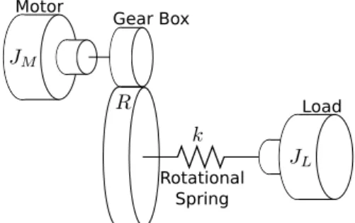
Figure 4: System considered for the actuator modeling.

the other is placed on the joint (#14), after the trans-mission chain. This layout measures the ratio and the deformation on the transmission and makes the model parameters theoretically observable.

Even though the flexible coupling should increase the transparency of the system, it seems to create constraints on the screw by preventing it to oscil-late freely. Moreover, contrary to (Garrec, 2010), the space around the cable (attached in the middle of the hollow screw with a crimped sleeve) is not sufficient, generating constraints in the mechanism. These con-straints create efforts and introduce non-linear and frictions depending on the actuator angular position (as detailed in Section 4.1).

2.2

Lagrangian Model

With respect to the mechanical description given be-fore, we use the following assumptions to construct the system model:

[A1] The DC motor driving the mechanism is con-sidered as a perfect source of torque.

[A2] Flexibilities are concentrated on a single linear rotational spring with constant stiffness.

Assumption [A1] is advisable as the motor is current controlled. Neglecting all magnetic loss the current is directly proportional to the motor output torque. We assume that the current controller is good and fast enough to provide our requested current command. Assumption [A2] is reasonable as the stiffness of the cable is several orders of magnitude lower than the stiffness of any other element in the transmission.

The actuator then boils down to a two-masses sys-tem attached by a spring, as illustrated in Fig. 4. The first mass is driven by a DC motor coupled with the gearbox. The second mass is interacting with the en-vironment. Friction arises in opposition to the motion of both masses.

Using Lagrangian formalism, we expose the fol-lowing model describing classical series elastic actu-ator. We empirically decided during the identification

experiments to consider viscious friction on both mo-tor and load side and dry friction on momo-tor side. JM¨θM= µKTiM− k R( θM R − q) − dM˙θM−Cfsign( ˙θM) (1a) JLq¨= τext+ k( θM R − q) − dLq˙ (1b) where the notations are given in Tab 1. In order to keep the equations smooth (as needed for the con-troller), we used a smooth version of the sign function (i.e. a hyperbolic tangent).

Table 1: Variables and parameters used in the model and corresponding values estimated on our system.

Symbol Physic meaning Identified value JM motor inertia 1.38× 10−5kg.m2

JL load inertia 8.5× 10−4kg.m2

θM motor angular position variable (rad)

q joint angular position variable (rad) k equivalent rotational spring stiffness 588 Nm/rad

R transmission ratio 96.1

τM motor torque variable (Nm)

τext external torque (environment) variable (Nm)

dM vicious friction at motor level 0.003 Nm/(rad/s)

dL vicious friction at load level 0.278 Nm/(ras/s)

C f dry friction at motor level 0.1 Nm KT motor current to torque ratio 60.3× 10−3Nm/A

µ motor efficiency 0.78

Because several mechanical phenomena were dif-ficult to model (see Section 4.1), we make the choice to keep a simple model. We could improve the model by identifying more precisely the frictions (coulomb, viscous and those depending on the angular position of the joint) as well as by more finely modelling the dynamics of the flexible elements (the system is com-posed of 2 flexible cables of different lengths, thus having 2 different dynamics). In practice, the good transparency of the gear make it possible to properly estimate the forces applied on the actuator. We can then rely on feedback more than on feedforward, be-ing given that the control law (hence the model) is sufficiently fast to be evaluated. The rational is the higher the control frequency, the lower error between the real system state and its estimation and the more accurate the control.

3

CONTROL

As reported in previous section, the actuator be-haves like a SEA transmission, with higher stiffness than typical SEA implementation. Different meth-ods can be used to handle these flexibilities, first by considering the actuator stiffness dynamics into the whole body problem formulation like it is done in (De Luca and Lucibello, 1998; Buondonno and

De Luca, 2016) for both series elastic or variable stiff-ness actuators. Another option is to neglect this dy-namic at the whole body level while handling it lo-cally at the joint level. In this section, we present the control solution that we implemented to track the joint reference, specified either as reference position or as reference torque. Our objective is then to compute the joint references from a whole-body optimization scheme, that will be accurately tracked by the joint controller running at high frequency.

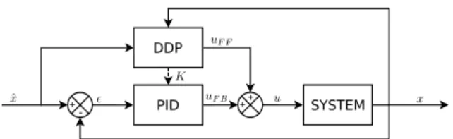
The controller we report below is composed of a two-stage architecture: a first stage, running on CPU at 1kHz, computes the optimal trajectory (feedfor-ward) and the optimal feedback gains in a model-predictive-control (MPC) style. The second layer, running on the micro-controller at higher frequency (5kHz or higher) uses the feedforward and the feed-back gains to compute the reference current sent to the motor. We start by a brief overview of possible control approaches that justifies our implementation based on differential dynamic programming (DDP).

3.1

Brief control state of the art

We are interested in setting up a controller either of the output joint position (position controller), or of the relative position of input and output (spring de-flection, i.e. force controller). In both cases, the ma-jor difficulty is the tuning of the control gains: high gains on position loop are necessary for good preci-sion but may make the system unstable due to the flexibility. Several control schema have been devel-oped to address this problem. The analysis of the Eigen modes of the actuator models to achieve de-sired convergence, stability and precision (Mehling, 2015; Paine et al., 2015) is difficult due to the model non-linear terms. Moreover, the same controller must be deployed on several variations of the same actua-tor implemented on the legs of Romeo. A more auto-matic method is desirable.

A method has been proposed in (Abroug and Laroche, 2015) to control SEA using H∞. It relies on

automatic controller tuning from identification data. However, the results that the controller is quite sen-sitive to identification errors, which makes it difficult to generalize. Alternatively, optimal control is very versatile (i.e. the controller can be quickly adapted to track either position or force references) and is quite resilient in practice to errors in the model (Sardellitti et al., 2013; Geoffroy et al., 2014). It is also straight-forward to generalize it to other SEA/VSA mecha-nisms, like pneumatic muscles (Das et al., 2016). Op-timal controller can also handle constraints like torque or position limits (Tassa et al., 2014). Optimal control

has been used to control both joint position and stiff-ness of an approximate linear model (LQR) (Sardel-litti et al., 2013). Dedicated approximations using polynomials have then been used to fit the computa-tion capabilities of the control board.

We rather propose here a two-stage approach to combine the versatility of the nonlinear optimal con-trol problem with the efficiency needed to solve it on the control board. The nonlinear problem is solved at medium frequency by the central CPU. The optimal control, along the corresponding Ricatti gains are then sent to the control board where the optimal control is updated from sensor measurements at high frequency. To keep the nonlinear solver simple while enforcing joint constraints, we implemented a box-DDP (Tassa et al., 2014), running at 1kHz. The control board then applies a PID corrector (using Ricatti gains extracted from the DDP) at 5kHz.

3.2

Differential dynamic programming

DDP is an optimal control scheme with a “single shooting” strategy, that is able to efficiently cope with the sparsity of the underlying numerical system but has the drawbacks of being quite unable to handle complex constraints. This trade-off is very suitable to our problem. We recall here the basis of DDP. This recall is needed for understanding how we designed both layers of our control architecture. More detailed information about this optimal control solver can be found in (Tassa et al., 2008).

Consider a generic mechanical system described by its (discrete) dynamic equation:

xi+1= fi(xi, ui) (2)

Where xi represents the current state of the actuator

(position, speed, torque ...) and uiis the input

com-mand (current, torque, voltage ...). This model may or not be linear and time varying. We expose the cost we want to minimize on a given horizon T .

J(U_|x0) = T−1

∑

respectively the state and control sequence over hori-zon T and x0the initial state of the system (typically

estimated from sensors). It is to be noticed that know-ing x0and U is enough to know the state of the system

at each moment of the horizon because of the rela-tion (2). So the optimal control problem consists in finding the correct U minimizing the cost for a given x0initial state.

We introduce then the cost-to-go function to be Ji(Ui|xi) =

T−1

∑

j=i

cj(xj, uj) + cT(xT) (4)

with xjintegrated from xi. The optimum cost-to-go is

named the value function V : V(x0, i) = min

Ui

Ji(x0, Ui) (5)

We obviously have that V (x0, T ) = cT(xT). The

“Bel-man” dynamic-programming principle teaches us that minimizing the cost by choosing the correct control sequence can be reduced to the backward minimiza-tion of a single control input. This principle gives us the Bellman equation :

V(xi, i) = min

u [ci(xi, ui) +V ( f (xi, ui), i + 1)] (6)

The DDP solver computes the optimal control sequence U by solving equation (6) backwardly in time. For this purpose let Q be the variation of c(x, u) + V ( f (x, u), i + 1) around the i− th state and command. We have :

Q(δx, δu)_{≡ c(x + δx,u + δu) − c(x,u)} +V ( f (x + δx, u + δu), i + 1)) −V ( f (x,u),i + 1))

(7)

By taking the second order approximation of (7) we obtain: Q(δx, δu)≈1₂   1 δx δu   T  0 QT_x QT_u Qx Qxx Qxu Qu Qux Quu     1 δx δu   (8) For readability we will use subscript notation to de-note partial derivative (e.g. fx= ∂ f (x,u)_∂x ). We also

denote the next state by V0_{≡ V (i + 1). We can now} expose: Qx = cx+ fxTVx0 (9) Qu = cu+ fuTVx0 (10) Qxx = cxx+ fxTVxx0 fx+Vx0fxx (11) Quu = cuu+ fuTVxx0 fu+Vx0fuu (12) Qux = cux+ fuTVxx0 fx+Vx0fux (13)

Where the last term of the last three equations repre-sents the contraction of a tensor with a vector. Mini-mizing (7) with respect to δu gives us:

δu∗= arg min

δu

Q(δx, δu) =−Q−1uu(Qu+ Quxδx) (14)

Showing up two terms:

• a feedforward term: k = −Q−1 uuQu

• a feedback term : K = −Q−1

uuQux

Using back this result into (7), we obtain a quadratic approximation of the value function at i_{−th instant:}

∆V (i) = −1 2QuQ −1 uuQu (15) Vx(i) = Qx− QuQ−1uuQux (16) Vxx(i) = Qxx− QuxQ−1uuQux (17)

Algorithm 1: Differential Dynamic Programming Solver 1: _{{initialisation :}}

2: U_{←random command sequence}

3: X_←init(x0, U) 4: repeat

5: V(T )_{← c}T(xT)

6: Vx(T )← cT x(xT) 7: Vxx(T )← cT xx(xT) 8: for i=T-1 down to 0 do

9: Qx, Qu, Qxx, Qu, Qux← see equations (9) to (13) 10: k_{← −Q}−1_uuQu 11: K_{← −Q}−1_uuQux 12: ∆V,Vx,Vxx← see equations (15) to (17) 13: end for 14: ˆx(0) = x(0) 15: for i=0 to T-1 do

16: ˆu(i) = u(i) + k(i) + K(i)(ˆx(i)_{− x(i))}

17: ˆx(i + 1) = fi(ˆx(i), ˆu(i)) 18: end for

19: until convergence

Computing all term from (9) to (17) for i = N_{− 1} down to i = 0 is called the backward phase. We then need to calculate the change induced on the state sequence by the modification on the command se-quence.

This is the forward phase, detailed below:

ˆx(0) = x(0) (18)

ˆu(i) = u(i) + k(i) + K(i)(ˆx(i)_{− x(i))(19)} ˆx(i + 1) = fi(ˆx(i), ˆu(i)) (20)

The solver iterates on these two phases until conver-gence of the result (minimal changes on U). One can find the algorithm detailed in a pseudo-code on algo-rithm 1.

In order to ensure good convergence and to add some specificities to the algorithm, we decided also to implement some other features:

Line search

DDP being a type of Newton descent, line search al-lows the algorithm to adapt the step length so that con-vergence is faster.

Regularization

DDP implies the inversion of Quu matrix which in

certain cases may not be invertible. Regularization makes the matrix invertible if it was not in the first place and it integrates this modification into the whole computation. SYSTEM PID DDP + + +

-Figure 5: General architecture of the proposed DDP-based MPC controller. The DDP running of CPU computes the optimal (feedforward) control uFF and the Ricatti gains K

at 1Khz. The control board (PID) then adds a feedback term uFBat 5Khz.

Control limitation

Introduced in (Tassa et al., 2014), the control limited DDP is an extension of the DDP where it is possible to add bound constraints on the command input vector. In practice this feature is possible by solving a box QP problem.

3.3

Two-stage control architecture

The outputs of the DDP solver are the optimal tra-jectories in both control U and state X spaces, along with the optimal feedback gains along this trajectory K. Our objective is to use at best this information to feedback as frequently as possible on the sensor mea-surements.

For that, we implement the DDP as a model-predictive (receding-horizon) control scheme. At any instant, we maintain a valid (possibly suboptimal) control trajectory U∗. As soon as the DDP performed one valid step of the nonlinear search loop (line #4 of Alg. 1), the solver candidate trajectory U is used to update U∗. The receding horizon of the DDP is then shifted, while the initial state of this new horizon is updated to the latest state estimation. The dynamic system considered in our DDP (1) is low-dimension and thus leads to short computation timings. It is easy to implement such solver to obtain 1kHz control fre-quency. However, it is difficult to implement the DDP solver directly on the actuator micro-controller, but rather on the central robot CPU board. The frequency is then limited by the communication bandwidth to upload the sensor measurements and download the control references.

On the other hand, the micro-controller of the ac-tuator is able to update the motor control at much higher frequency (e.g. 5kHz). This higher frequency enables us to take advantage of the optimal feed-back gains computed by the DDP solver. On the micro-controller, we then maintain an optimal con-trol (feedforward) trajectory and the corresponding optimal feedback gains along this trajectory. At each

0 1 2 3 4 5 time (s) −0.2 0.0 0.2 0.4 0.6 0.8 1.0 1.2 1.4 1.6 joint angle (r ad) Estimation Measurements

Figure 6: Comparison between model and real system re-sponse to a same control input (motor current).

control cycle of the micro-controller, the state is esti-mated from previous sensor measurements. The con-trol (reference motor current i∗) is then computed as the sum of the feedforward (optimal control u∗) and feedback (optimal gains K∗):

i∗(t) = u∗(t) + K∗(x∗(t)_{− ˆx(t))}

where x∗ is the latest optimal trajectory in the state space computed by the DDP and ˆxis the estimated state.

Fig. 5 shows the general architecture of the pro-posed controller. The DDP controller runs at 1kHz on CPU and produces the feedforward control uFF. The

feedback controller runs at 5kHz on micro-controller, estimates the state and produces the feedback control uFB from the optimal gains K. The communication

bus between micro-controller and CPU board carries the estimated state at 5kHz and the optimal feedfor-ward and gains at 1kHz. Both feedforfeedfor-ward and feed-back are finally summed and used to servo the motor current.

4

SIMULATION AND

EXPERIMENTS

4.1

Actuator parameters estimation

Off-line estimation: All measurements (joint po-sition, motor popo-sition, motor current, motor supply voltage ...) are collected while controlling the actu-ator with a simple controller (PID with low gains). The estimation of the model parameters is done using MATLAB R_{. The result is shown in Fig. 6, by} com-paring simulated and hardware response to a same open-loop control. Thanks to the transparency of the actuator, the model is easily identified. The predic-tion in simulapredic-tion properly fits with the real trajectory.

1.0 1.2 1.4 1.6 1.8 2.0 2.2

joint angular position (rad)

0 5 10 15 20 25 torque (Nm) 1.0 1.2 1.4 1.6 1.8 2.0 2.2

joint angular position (rad)

0 5 10 15 20 25

Figure 7: Output joint torque estimation: (left) using only the two joint encoders measuring the spring deflec-tion (right) using the current measures and the full actuator model. The estimation from encoders is biased by the fric-tion in the hardware. The current measure leads to a quite good torque estimation although noisy. Both measures are satisfactory given the absence of a direct torque sensor, and are complementary. Each color represents a different output load (masses attached to the actuator output).

Although the parameters are better estimated than on other types of transmission, the identification is not perfect. From the captured data, we identified that this comes from several defects in the implementa-tion of the actuator (ball-screw being too much con-strained by the flexible coupling, cable being not free enough at the mounting with the ball-screw, elasticity being different in the two directions due to the un-equal length of the two cables). It would be possible to model these effects, hence to obtain a better pre-diction. However, it would also make the controller more complex and more costly. We rather believe that it would be easier to correct this effect by a more care-ful implementation of the actuator.

On-line estimation: The actuator is not equipped with direct torque sensor. However, two indirect mea-surements are available. We have two encoders on each side of the flexibility, and can then use the model to estimate the output torque. Thanks to the actua-tor transparency, we can also use the measured mo-tor current to estimate the output mo-torque. To validate both measurements, we took measurements points for different joint positions in a static state with different known masses attached to the actuator output. The mass being static, the output torque is known and can be compared to the estimation using either the en-coders or the current sensor. The result is displayed in Fig. 7. Both estimations are accurate. They also are complementary: the estimation from the encoders is biased by friction; the estimation from current is more

0.4 0.6 0.8 1.0 1.2 1.4 1.6 1.8 2.0 time (s) −0.2 0.0 0.2 0.4 0.6 0.8 1.0 1.2 joint angle (r ad) simulation (ideal) feedforward only (biased) feedback only (biased) feedforward + feedback (biased)

Figure 8: Simulation for ideal and biased model with feed-forward and/or feedback (similar trajectories are obtained when a single term is active).

noisy. Merging both estimations in a proper estimator would lead to an accurate estimation able to compete with a direct torque measurement (without the price, implementation issue and fragility of an actual torque sensor).

In conclusion, the transparency of the actuator leads to accurate model estimation, both for (off-line) calibration and (on-line) torque estimation.

4.2

Experiments - position control

Simulation:We validate first the position controller in simulation, using the model and the two-stage MPC presented above. The MPC uses the true (identified) model for prediction, while the simulation is inte-grated using a biased model (parameters randomly modified of 50% – for convenience we only plot re-sults for a single biased model). Control frequencies are the same as on the real system. Fig. 8 displays the effect of the feedback and feedforward terms for a step input. The reference is accurately tracked. The steady state is quickly reached because the actuator is quite stiff. By mixing feedback and feedfoward, the MPC offers a good robustness to modeling errors.

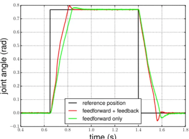
Hardware experiments: The same experiments have been made on the real system. Results are dis-played on Fig. 9 and 10. The reference is properly tracked, with the steady state being reached with a time similar to the ideal case. As in simulation, mix-ing feedforward and feedback helps to obtain a better behavior. On the hardware, the modeling errors are more significant than with the simulated models (due to non modeled effects as already mentioned, like pe-riodic friction, etc). The box-DDP is useful in this case to prevent current overshoot in the motor (e.g. between 0.8s and 1.5s). Finally, we show in Fig. 11

0.4 0.6 0.8 1.0 1.2 1.4 1.6 1.8 time (s) −0.1 0.0 0.1 0.2 0.3 0.4 0.5 0.6 0.7 0.8 joint angle (r ad) reference position feedforward + feedback feedforward only

Figure 9: Hardware experiment: position tracking with and without feedforward (feedback must be alsways active on hardware). 0.4 0.6 0.8 1.0 1.2 1.4 1.6 1.8 time (s) −6 −4 −2 0 2 4 6 current (A)

Motor current command

Figure 10: Hardware experiment: motor current when tracking a step position.

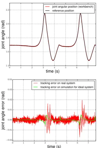
the results of tracking a realistic trajectory, taken from a walking movement generated with a pattern gen-erator (trajectory of the knee of robot HRP-2 during 15cm stair climbing). The trajectory is very dynamic. the first figure shows the reference joint trajectory as well as the actual follow-up performed by the actua-tor controlled using our method. The curves are very close, the average error is less than 1%. The error (difference between the desired position and the ac-tual position of the system) is displayed on the second figure in simulation and on the actual system. This error remains very small and increases during sudden changes of direction (dynamic movements).

4.3

Experiments - torque control

We also validate the torque controller, in simulation only. Results are shown in Fig. 12. We again observe the response of the controller to a step input. As

be-0 1 2 3 4 5 6 7 time (s) 1.4 1.6 1.8 2.0 2.2 joint angle (r ad)

joint angular position (workbench) reference position 0 1 2 3 4 5 6 7 time (s) −0.02 −0.01 0.00 0.01 0.02 0.03 0.04 joint angle error (r ad)

tracking error on real system

tracking error on simulation for ideal system

Figure 11: Tracking a dynamic position trajectory. (up) Reference and actual trajectories (down) Tracking error. Less than 1% error in average was observed.

fore, the analysis is achieved while disturbing the pa-rameters of the model used in simulation while keep-ing the same MPC model. With a perfect model, the steady state is perfectly reached. The time to steady state is shorter than with the position controller, as expected. When bias is added, we keep a similar be-havior but the reference is not perfectly reached any-more. As we do not have a direct (non biased) esti-mation of output torque, this would not be possible. However, we also see that the behavior remains good despite the bias and that improving the estimation of the model parameters (in particular the stiffness) on-line based on any external measurement of the output torque would be quite easy.

5

CONCLUSION

In this paper, we have presented the complete im-plementation of a new compact, high-gear and trans-parent actuator, very suitable for mobile robots, in

0.0 0.2 0.4 0.6 0.8 1.0 1.2 1.4 1.6 1.8 time (s) −0.5 0.0 0.5 1.0 1.5 2.0 2.5 3.0 joint

torque(Nm) _{ideal model}

10% biased model 20% biased model 50% biased model 80% biased model trajectory reference

Figure 12: Torque control of the actuator in simulation for ideal and biased models with several levels of bias.

particular in the context of locomotion, with identifi-cation and an original two-stage control scheme. The optimal controller is lightweight, easy to implement, and can compute a feedback at 5kHz on a micro-controller board. We have shown in the experiment results that both layers are needed to efficiently con-trol the actuator: either feedforward or feedback alone are not able to perform as efficiently. Moreover, we experimentally showed the capabilities of the actuator in term of transparency (i.e. estimating output torques from motor current), and the adequacy of the model to capture the complexity of the actuator.

The main result of this study is that the actuator with our control scheme offers very good property, which makes it very suitable to replace strain-wave gears in electric actuation of humanoid robots. In particular, it offers full backdrivability (hence more efficiency, less dangerousness and more chock re-sistance) and accurate estimation of the output joint torque without direct measurement (i.e. no force sen-sor needed).

While the proposed control architecture is very suitable for the screw-nut-cable actuator, it is also ap-propriate for other kind of flexible actuators such as SEA at large, variable stiffness actuators (Sardellitti et al., 2013) or Mckibben pneumatic actuators (Das et al., 2016). The MPC scheme can be easily adapted to another dynamic model or another cost function. Our objective is now to adapt the controller to the whole body of the robot and to use it to control com-plex humanoid movements.

ACKNOWLEDGMENT

This work was partially funded by the FLAG-ERA JTC project ROBOCOM++, which aims at re-thinking robotics for the robot companion of the fu-ture.

REFERENCES

Abroug, N. and Laroche, E. (2015). Transforming se-ries elastic actuators into variable stiffness actua-tors thanks to structured h∞control. In European

Control Conference (ECC), pages 734–740. Alfayad, S., Ouezdou, F. B., Namoun, F., and Gheng,

G. (2011). High performance integrated electro-hydraulic actuator for robotics–part i: Principle, prototype design and first experiments. Sensors and Actuators A: Physical, 169(1):115–123. Buondonno, G. and De Luca, A. (2016).

Effi-cient computation of inverse dynamics and feed-back linearization for vsa-based robots. IEEE Robotics and Automation Letters, 1(2):908–915. Das, G.-K.-H.-S.-L., Tondu, B., Forget, F., Manhes, J., Stasse, O., and Soueres, P. (2016). Con-trolling a multi-joint arm actuated by pneumatic muscles with quasi-ddp optimal control. In IEEE/RSJ Int. Conf. on Intelligent Robots and Systems (IROS), pages 521–528.

De Luca, A. and Lucibello, P. (1998). A general al-gorithm for dynamic feedback linearization of robots with elastic joints. In IEEE/RAS Int. Conf. on Robotics and Automation (ICRA), volume 1, pages 504–510. IEEE.

Englsberger, J., Werner, A., Ott, C., Henze, B., Roa, M. A., Garofalo, G., Burger, R., Beyer, A., Eiberger, O., Schmid, K., et al. (2014). Overview of the torque-controlled humanoid robot toro. In IEEE/RAS Int. Conf. on Humanoid Robots (Hu-manoids), pages 916–923. IEEE.

Garrec, P. (2010). Design of an anthropomorphic up-per limb exoskeleton actuated by ball-screws and cables. Bulletin of the Academy of Sciences of the Ussr-Physical Series, 72(2):23.

Geoffroy, P., Bordron, O., Mansard, N., Raison, M., Stasse, O., and Bretl, T. (2014). A two-stage suboptimal approximation for variable compli-ance and torque control. In Control Conference (ECC), 2014 European, pages 1151–1157. Lee, J., Choi, W., Kanoulas, D., Subburaman, R.,

Caldwell, D. G., and Tsagarakis, N. G. (2016). An active compliant impact protection system for humanoids: Application to walk-man hands.

In IEEE/RAS Int. Conf. on Humanoid Robotics (ICHR), pages 778–785.

Mehling, J. S. (2015). Impedance Control Ap-proaches for Series Elastic Actuators. PhD the-sis, Rice University.

Paine, N., Mehling, J. S., Holley, J., Radford, N. A., Johnson, G., Fok, C.-L., and Sentis, L. (2015). Actuator control for the nasa-jsc valkyrie hu-manoid robot: A decoupled dynamics approach for torque control of series elastic robots. Jour-nal of Field Robotics, 32(3):378–396.

Pratt, G. A. and Williamson, M. M. (1995). Series elastic actuators. In IEEE/RSJ Int. Conf. on In-telligent Robots and Systems (IROS), volume 1, pages 399–406.

Sardellitti, I., Medrano-Cerda, G. A., Tsagarakis, N., Jafari, A., and Caldwell, D. G. (2013). Gain scheduling control for a class of variable stiff-ness actuators based on lever mechanisms. IEEE Transactions on Robotics, 29(3):791–798. Semini, C., Tsagarakis, N. G., Guglielmino, E.,

Foc-chi, M., Cannella, F., and Caldwell, D. G. (2011). Design of hyq–a hydraulically and elec-trically actuated quadruped robot. Proceedings of the Institution of Mechanical Engineers, Part I: Journal of Systems and Control Engineering, 225(6):831–849.

Tassa, Y., Erez, T., and Smart, W. D. (2008). Reced-ing horizon differential dynamic programmReced-ing. In Advances in Neural Information Processing Systems 20, pages 1465–1472.

Tassa, Y., Mansard, N., and Todorov, E. (2014). Control-limited differential dynamic program-ming. In IEEE/RAS Int. Conf. on Robotics and Automation (ICRA), pages 1168–1175.

Wensing, P. M., Wang, A., Seok, S., Otten, D., Lang, J., and Kim, S. (2017). Proprioceptive actuator design in the mit cheetah: Impact mitigation and high-bandwidth physical interaction for dynamic legged robots. IEEE Transactions on Robotics. Wolf, S. and Hirzinger, G. (2008). A new variable

stiffness design: Matching requirements of the next robot generation. In IEEE/RAS Int. Conf. on Robotics and Automation (ICRA), pages 1741– 1746. IEEE.