HAL Id: tel-02280155
https://tel.archives-ouvertes.fr/tel-02280155
Submitted on 6 Sep 2019
HAL is a multi-disciplinary open access
archive for the deposit and dissemination of
sci-entific research documents, whether they are
pub-lished or not. The documents may come from
teaching and research institutions in France or
abroad, or from public or private research centers.
L’archive ouverte pluridisciplinaire HAL, est
destinée au dépôt et à la diffusion de documents
scientifiques de niveau recherche, publiés ou non,
émanant des établissements d’enseignement et de
recherche français ou étrangers, des laboratoires
publics ou privés.
statistical-physics approach to neural attractors and
protein fitness landscapes
Lorenzo Posani
To cite this version:
Lorenzo Posani. Inference and modeling of biological networks : a statistical-physics approach to
neural attractors and protein fitness landscapes. Physics [physics]. Université Paris sciences et lettres,
2018. English. �NNT : 2018PSLEE043�. �tel-02280155�
A C K N O W L E D G M E N T S
We all are products of our environment, and this thesis is no exception. During these three years I had the privilege to work alongside exceptional mentors and peers, whose ideas and suggestions pervade this manuscript on many levels.
I first must express my gratitude to Simona Cocco and Rémi Monasson for taking the commitment of managing my "non-orthodox" working hours both as a master student and as a Ph.D. candidate. The transition from "learning" to "doing" science can be harsh for students, but you both sweetened the deal by providing a brilliant example of how professional scientists think and work, and I will always be grateful for that.
My warm and sincere thanks go to my brothers-in-thesis, Marco Molari and Jerome Tubiana, who did not miss one single occasion to prove their kindness and will to help, equaled only by the sharpness of their mind. You really made me feel like home, which probably explains the unhealthy frequency of dinner at the office together! Special thanks are also due to Diego Contreras, who taught me bike and philosophy (unrelatedly), Kevin Berlemont, Clement Roussel, and Max Puelma Touzel for helping me with French and English, respectively, and Francesca Rizzato with whom I had the pleasure to collabo-rate on the protein fitness landscape project and whose results are partially included here. Big thanks are due to all my colleagues and friends for making the ENS (and, more generally, Paris) such a stimulating and enjoyable environment, each with his/her pe-culiar character and mind. In pseudo-order of appearance: Gaia Tavoni, Alice Coucke, Tommaso Brotto, Tommaso Comparin, Anirudh Kulkarni, Quentin Feltgen, Volker Per-nice, Manon Michel, Ze Lei, Tridib Sadhu, Juliane Klamser, Alexis Dubreuil, Andreas Mayer, Louis Brezin, Elisabetta Vesconi, Ivan Amelio, Quentin Marcou, Tran Huy, Jacopo Marchi, Cosimo Lupo, Victor Dagard, Michelangelo Preti, Aldo Battista, Eduarda Susin, Sebastien Wolf, Moshir Agarwal, Ohgod Youaresomany, Daniele Conti, Giulio Isacco, Federica Ferretti, Fabio Manca, Arnaud Fanthomme, Simone Blanco Malerba , Silvia Ferri, and all those who I may have forgotten, who will not take it personally since they are familiar with my total lack of episodic memory.
Finally, I’d like to dedicate a word to my life partner and lifeblood, Federica, who constantly supported me with her piercing intelligence and unconditioned tenderness. You enlightened every single step of this three-years journey, which would have been impossible without you by my side. Words can not express how thankful I am.
A B S T R A C T
The recent advent of high-throughput experimental procedures has opened a new era for the quantitative study of biological systems. Today, electrophysiology recordings and calcium imaging allow for the in vivo simultaneous recording of hundreds to thousands of neurons. In parallel, thanks to automated sequencing procedures, the libraries of known functional proteins expanded from thousands to millions in just a few years. This current abundance of biological data opens a new series of challenges for theoreticians. Accurate and transparent analysis methods are needed to process this massive amount of raw data into meaningful observables. Concurrently, the simultaneous observation of a large number of interacting units enables the development and validation of theoretical models aimed at the mechanistic understanding of the collective behavior of biological systems. In this manuscript, we propose an approach to both these challenges based on methods and models from statistical physics.
The first part of this manuscript is dedicated to an introduction to the statistical physics approach to systems biology, with a particular focus on the interfaces between statistical physics, Bayesian inference, and systems biology. The intersections between these fields are presented by following the common thread of the tools and models that have been applied, during the development of this thesis, to the study of two biological systems: the navigation-memory task in the hippocampal complex (part II) and the fitness landscape of co-evolving residues in proteins (part III).
The second part is dedicated to the representation of navigation memory in the hip-pocampal network. We first introduce a Bayesian population-activity decoder, based on the adaptive cluster expansion (ACE) of the graphical-Ising inference, aimed at retrieving the represented cognitive map on fast time scales. We apply the decoder on CA1 data, showing that it outperforms the current standards in discriminating the recalled cognitive state, and on in-silico data, to investigate the functional meaning of the inferred neural couplings. We then apply this method to the investigation of the flickering phenomenology, i.e., the oscillatory behavior of the cognitive map that was observed in a recent experiment where contextual cues are abruptly changed to induce the network instability in the rodent hippocampal region CA3. We present an attractor model, subject to external and path-integrator inputs, which is shown to accurately reproduce the oscillating phenomenology of the cognitive map. By the application of the Ising decoder, we show that a number of novel predictions of the model, concerning the precision of the positional representation during the instability of the cognitive state, can be verified by a careful re-analysis of the original data. Finally, we show that the Ising model inferred from hippocampal recordings can be used to generate population activities that are coherent with low-dimensional attractors, which have been proposed as the neural mechanism underlying spatial navigation in the cognitive map.
In the third part, we employ a statistical-physics model of protein folding, called Lattice Proteins, to benchmark inference methods aimed at the reconstruction of the local fitness landscape of a protein from sequence data of homologous proteins. We first show that a sparse version of the ACE inference, which adapts the sparsity of the inferred interaction graph to the number of available data, yields superior performances than standard DCA methods in the common sub-sampled regime. We then frame the inference task in the context of the bias-variance trade-off, showing that we can optimize its retrieval performance by choosing the proper subset of the training alignment (MSA). We propose a procedure, called "focusing," aimed at finding this optimal subset from a given MSA, opening to applications on real protein datasets.
R E S U M É
L’avènement récent des procédures expérimentales à haut débit a ouvert une nouvelle ère pour l’étude quantitative des systèmes biologiques. De nos jours, les enregistrements d’électrophysiologie et l’imagerie du calcium permettent l’enregistrement simultané in vivo de centaines à des milliers de neurones. Parallèlement, grâce à des procédures de séquençage automatisées, les bibliothèques de protéines fonctionnelles connues ont été étendues de milliers à des millions en quelques années seulement. L’abondance actuelle de données biologiques ouvre une nouvelle série de défis aux théoriciens. Des méthodes d’analyse précises et transparentes sont nécessaires pour traiter cette quantité massive de données brutes en observables significatifs. Parallèlement, l’observation simultanée d’un grand nombre d’unités en interaction permet de développer et de valider des modèles théoriques visant à la compréhension mécanistique du comportement collectif des systèmes biologiques. Dans ce manuscrit, nous proposons une approche de ces défis basée sur des méthodes et des modèles issus de la physique statistique.
La première partie de ce manuscrit est consacrée à une introduction de l’approche des systèmes biologiques par la physique statistique. Dans cette partie, l’accent est porté sur l’interface entre la physique statistique, l’inférence bayésienne et les systèmes biologiques. Les intersections entre ces domaines sont présentées en suivant le fil conducteur des outils et modèles qui ont été appliqués, lors de cette thèse, à l’étude de deux systèmes biologiques particuliers : la tâche navigation et mémoire spatiale dans le complexe hippocampique (partie II) et le paysage adaptatif de coévolution dans les protéines (partie III).
La deuxième partie est consacrée à la représentation de la mémoire spatiale dans le réseau hippocampique. Nous introduisons d’abord un décodeur Bayésien d’activité de population, basé sur l’expansion adaptative de clusters (ACE) de l’inférence d’un modèle d’Ising sur un graph, visant à récupérer la carte cognitive représentée sur des échelles de temps rapides. Nous appliquons le décodeur sur des données CA1, montrant qu’il surpasse les normes actuelles en matière de discrimination de l’état cognitif rappelé, et sur des données in-silico, pour étudier la signification fonctionnelle des couplages neuronaux inférés. Nous appliquons ensuite cette méthode à l’étude de la phénoménologie du « flickering », c’est-à-dire le comportement oscillatoire de la carte cognitive observé lors d’une expérience récente où les conditions contextuelles sont brusquement modifiées pour induire l’instabilité du réseau dans la région hippocampique CA3 du rongeur. Nous présentons un modèle d’attracteur, soumis à des entrées externes et à des intégrateurs de trajectoire, dont il est démontré qu’il reproduit avec précision la phénoménologie oscillante de la carte cognitive. Par l’application du décodeur précédent, nous montrons qu’un certain nombre de nouvelles prédictions du modèle, concernant la précision de la représentation positionnelle pendant l’instabilité de l’état cognitif, peuvent être vérifiées par une nouvelle analyse des données originales. Enfin, nous montrons que le modèle
d’Ising inféré des enregistrements de l’hippocampe peut être utilisé pour générer des activités de population cohérentes avec les attracteurs de faible dimension, qui ont été proposés comme mécanisme neuronal sous-jacent à la navigation spatiale dans la carte cognitive.
Dans la troisième partie, nous employons un modèle de physique statistique du repliement des protéines, appelé « Lattice Proteins », pour comparer les méthodes d’inférence visant à reconstruire le paysage adaptatif local d’une protéine à partir des données de séquence des protéines homologues. Nous montrons d’abord qu’une ver-sion éparse de l’inférence ACE, qui adapte la rareté du graphique d’interaction inféré au nombre de données disponibles, donne des performances supérieures à celles des méthodes DCA standard dans le régime commun sous-échantillonné. Ensuite, dans le contexte du dilemme biais-variance, nous montrons que nous pouvons optimiser le rendement de récupération de notre inférence en choisissant le sous-ensemble approprié de l’alignement des protéines (MSA). Nous proposons une procédure, appelée « focusing », visant à trouver ce sous-ensemble optimal à partir d’un alignement donné. Cette procédure pourrait avoir des applications sur des ensembles de protéines réelles.
P U B L I C AT I O N S
This manuscript comprises the research work that I have conducted during the last three years under the supervision of Simona Cocco and Rémi Monasson at the Laboratoire de Physique Statistique de l’Ecole Normale Superieure, and includes published as well as original results.
For what concerns the hippocampus part, Chapters 5 and 6 have been published as research papers in [1, 2], in collaboration with Karel Ježek from Charles University (Prague). Some of the early results of Chapter 6 were presented at [3]. Part of the ideas and results showed in Chapter 4 have been included in [4, 5]. Chapter 7 is a work in progress at the draft stage [6].
Chapters 9, 10, and 11 present an analysis of inference models applied to the retrieval of the mutational landscape of a protein from sequence data. While these chapters mostly cover results obtained on theoretical models, this work was conducted in parallel with a postdoctoral researcher, Francesca Rizzato, who applied similar analyses to real protein datasets. The results of this collaboration will be jointly published in two future papers, now at the draft stage [7, 8].
Publications
[1] L. Posani, S. Cocco, K. Ježek, and R. Monasson, “Functional connectivity models for decod-ing of spatial representations from hippocampal ca1 recorddecod-ings,” Journal of Computational Neuroscience, pp. 1–17, 2017.
[2] L. Posani, S. Cocco, and R. Monasson, “Integration and multiplexing of positional and contextual information by the hippocampal network,” PLoS computational biology, vol. 14, no. 8, p. e1006320, 2018.
Review papers, conference proceedings
[3] L. Posani, S. Cocco, K. Ježek, and R. Monasson, “Position is coherently represented during flickering instabilities of placecell cognitive maps in the hippocampus,” BMC neuroscience
-26th Annual Computational Neuroscience Meeting (CNS* 2017), vol.18-1, pp.58, 2017.
[4] S. Cocco, R. Monasson, L. Posani, and G. Tavoni, “Functional networks from inverse modeling of neural population activity,” Current Opinion in Systems Biology, 2017.
[5] S. Cocco, R. Monasson, L. Posani, S. Rosay, and J. Tubiana, “Statistical physics and representa-tions in real and artificial neural networks,” Physica A: Statistical Mechanics and its Applicarepresenta-tions, p. doi/10.1016/j.physa.2017.11.153, 2017.
In preparation
[6] L. Posani, S. Cocco, and R. Monasson, “Pairwise models inferred from hippocampal activity generate neural configurations typical of single or multiple low-dimensional attractors,” 2018. [7] L. Posani†, F. Rizzato†, R. Monasson, and S. Cocco, “Infer global, predict local: Bias-variance trade-off in protein fitness landscape reconstruction from sequence data,” 2018 (†: joint first authors)
[8] L. Posani†, F. Rizzato†, R. Monasson, and S. Cocco, “Improved performance of DCA fitness predictions with sparsity prior from structural information,” 2018 (†: joint first authors)
C O N T E N T S
i statistical physics, inference, biology: an intriguing scientific braid
1 background 15
1.1 Statistical Physics 15
1.1.1 The Boltzmann approach 16
1.1.2 Boltzmann entropy and Helmholtz free energy 18 1.1.3 The Gibbs approach 19
1.2 Bayesian Inference 21 1.2.1 Extended logic 21 1.2.2 The Bayes theorem 22 1.2.3 Hypothesis testing 23
1.2.4 Maximum likelihood and maximum a posteriori 23 1.2.5 The "max-entropy" principle 25
2 intersections 27
2.1 Bayesian Inference\Statistical Physics 28 2.1.1 The inverse Ising model 28 2.1.2 Sparsity and regularization 30 2.1.3 Computational approaches 31 2.2 Statistical Physics\Systems Biology 36
2.2.1 Biology is complicated 36 2.2.2 Biology is complex 37
2.2.3 Simple models of complex systems 37
ii navigation and memory in the hippocampal complex: modelling and inference of attractors from neural recordings
3 background 43
3.1 Navigation and memory in the hippocampus 43 3.1.1 The hippocampus 43
3.1.2 Place cells 44
3.1.3 Head-direction cells 45
3.1.4 Grid cells and path integration 45
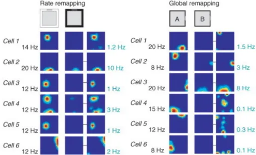
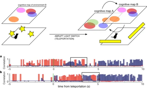
3.1.5 What inputs drive the firing of place cells? 47 3.1.6 The "teleportation" experiment 48
3.2 Memory and Attractor Neural Networks 50 3.2.1 The Hebbian theory of memory 50 3.2.2 The Hopfield model 50
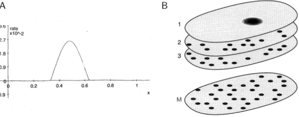
3.2.3 CANN: Continuous-Attractor Neural Network 51 3.3 Outline of the following chapters 52
4 inferring the attractor state from population activity: the "subsampling" problem 55
4.1 Introduction 55
4.2 Methods 56
4.3 Results 62
5 decoding the cognitive map in ca1 with ising inference 67 5.1 Introduction 68
5.2 Results 70 5.3 Discussion 80
5.4 Methods 83
5.5 Supplementary Information 90
6 investigation of the "flickering" phenomenology in ca3 93 6.1 Introduction 94
6.2 Results 96 6.3 Discussion 106 6.4 Methods 109
7 the generative power of the inferred ising model 115 7.1 Introduction 115
7.2 Attractor-like behavior of the inferred model: single map 116 7.3 Attractor-like behavior of the inferred model: two maps 121
iii infer global, predict local: bias-variance trade-off in protein fitness landscape reconstruction from sequence data
8 background 127
8.1 Direct-coupling analysis (DCA) from sequence data 127 8.1.1 The inverse Potts model 127
8.1.2 Contact prediction 128 8.1.3 Fitness prediction 129 8.1.4 Open issues 131 8.2 Lattice Proteins 132
8.2.1 The model 132
8.2.2 Sampling an MSA from a Lattice Protein family 134 8.3 Outline of the following chapters 136
9 the mutational landscape of lattice proteins 137
9.1 Dispersion of the mutational landscape depends on the fitness 137 9.2 Derivation of s⇠ (1 Pnat)scaling 138
9.3 Relationship between Potts and real landscapes depends on the fitness 141 10 sparse potts inference with structural prior (sp-ace) 147
10.1 Introduction 147 10.2 Results 148 10.3 Discussion 154 10.4 Methods 155
contents 11
11 the focusing procedure: select the optimal training msa for fitness predictions 159
11.1 Introduction 159
11.2 Bias-variance tradeoff in independent-Potts inference 160 11.3 The "focusing" procedure: Independent model 169 11.4 Bias-variance tradeoff in Structural-Potts inference 173 11.5 The "focusing" procedure: cmap-ACE Potts model 175 11.6 Scaling law in real protein datasets 179
11.7 Discussion 180
iv conclusions
12 discussion and perspectives 183 12.1 Outline 183
12.2 Methodology and future research 184
v appendix
a appendix - chapter 6 189
a.1 Effective two-state model for hippocampal CANN activity 189 a.2 Effects of parameters on the model properties 190
a.3 Relationship between sojourn time and correlation time 194
a.4 Inference of path-integrator realignment times - discussion on parameters p0and pe 195
a.5 Independence of frequency of flickers from delay after light switch: pa-rameters p0and peand L0 196
a.6 Assessment of performances of map decoder 197 a.7 Dependence of positional-error analysis with L0 199 b appendix - chapter 11 201
Part I
S TAT I S T I C A L P H Y S I C S , I N F E R E N C E , B I O L O G Y: A N I N T R I G U I N G S C I E N T I F I C B R A I D
1
B A C K G R O U N D1.1 statistical physics
Statistical physics, as the name suggests, is the branch of physics that deals with the statistical analysis of physical phenomena. It finds its roots in the kinetic theory of thermodynamics, developed mainly by James Clerk Maxwell and Ludwig Boltzmann in the 19th century, and later significantly contributed to by Willard Gibbs with his seminal work "Elementary principles in statistical mechanics" [9].
In some sense, statistical physics represents an answer to the analytical intractability of many-body systems. As proven by the famous work of Henry Poincaré in 1887 [10], a detailed deterministic description of the motion of three (or more) bodies, interacting through Newton’s laws of gravitation, is impossible, since the system follows a chaotic (non-periodic) dynamics in the phase space.
However, some systems, such as gases, crystals, and amorphous solids, display a limited number of stable macroscopic behaviors, even though they are composed of a massive amount of interacting bodies (atoms or molecules). This apparent paradox is elegantly solved by the concept of statistical equilibrium: even though the single molecule of air follows a chaotic and fast dynamics, endlessly moving at an average speed of
⇠400m/s, it is very unlikely (statistically) that a significant number of molecules will coherently move to the same direction, creating a spontaneous flow of air to one side of the room. As a result, the ensemble, or gas, is globally static, and the room is always uniformly filled by breathable air.
Statistical physics (of equilibrium) deals with many-body systems where the number of interacting units, and the nature of the interaction, is such that the global behavior of the system displays a limited number of stable equilibrium conditions. In these cases, one can derive an analytical picture, at the ensemble level, by giving up the microscopic determinism and introducing uncertainty - therefore statistics - in the theory.
To that end, the conceptual approach of statistical physics is to explain the phenomenol-ogy of a macroscopic object by deriving a macroscopic theory from the detailed laws that rule the behavior of its microscopic components.
The power of this approach lies in its generality: for the right set of phenomena, the global behavior of the ensemble does not depend of the detailed nature of its constitutive elements. Therefore, for example, the theory developed for the formation of droplets during liquid-vapor transition [11] can also be used to describe the self-sustained neural activity that encodes a spatial position in the collective state of a neural population [12]. As we will see in the next chapters, this generality has been leveraged by many (often successfully) to apply the tools of statistical physics to a wide variety of fields.
1.1.1 The Boltzmann approach
One of the pillars of statistical physics is the so-called Boltzmann distribution, which relates the probability for a system to be in a state to the energy of the state and the temperature. We will here review the derivation due to Boltzmann himself: the law was derived to describe the distribution of energy within a gas composed of a large number of molecules in a thermal bath, and was first given in his paper dated 1877 (see [13] for an English translation).
Let’s consider an isolated idealized system composed of N interacting particles, each having kinetic energy eiwith i2 [1, N]. Globally, the total energy E is conserved, but particles can hit each other and exchange their energy by elastic collisions. Therefore, in time, the individual values of eiwill vary due to the continuous scattering happening at the microscopic level. The system is described by a chaotic trajectory of the 6N-dimensional phase space vector
z(t) = (q1(t), . . . , qN(t), p1(t), . . . , pN(t)) ,
where qi(t)and pi(t)are the three-dimensional space position and three-dimensional momentum of the i-th particle.
Boltzmann started with a simplification: each eican take only a set of discrete values, and the exchanges happen accordingly via discrete amounts of an elementary unit e. Therefore, at any time we have
ei=aie ,
were each a is limited by 0 (below) and by the total energy E=Le (above), and varies with time due to collisions. This is the equivalent of making a coarse-grained partition of the phase space into cells of finite size. The variable z(t), therefore, moves within this discrete (although huge) set of states. Each of this cells is called a microstate. A fundamental hypothesis is that the system occupies each microstate with equally probability, called the ergodic hypothesis. Boltzmann then focused on the question of how the energy is distributed within the system, i.e., how many particles have energy ei=0, e, 2e and so on. To do so, he performed a change of variable: instead of considering the microscopic kinetic state of the whole system z(t), he considered the occupation vector
n= (n0, n1, . . . , nL) ,
where na is the number of molecules that have energy ae. Now, it is clear that the coordinate change is not bijective, in the sense that each occupation vector corresponds to a different number of microstates in the phase space. The occupation vector is, therefore, a macrostate, i.e., a state of the system that corresponds to an entire region of the phase space. In the ergodic hypothesis, every microstate is equally probable. Therefore we can compute the relative probability of macrostates by just counting how many microstates map to each of them, i.e., computing the corresponding phase-space volume. We call this
1.1 statistical physics 17
number W(n). To compute it, let’s proceed iteratively: given an occupation vector n, we have, out of N atoms,
✓ N n0 ◆
= N!
(N n0)!n0!
ways of choosing n0molecules to whom assign the energies e=0. We then are left with N n0molecules, and we choose n1out of them to pick the molecules with energy e=e, so we multiply by(N n0 n1 ). N! (N n0)!n0! (N n0)! (N n0 n1)!n1! = N! n0!n1! 1 (N n0 n1)!
Proceeding this way, we see that the N n0 n1. . . term is simplified at each step, until the final solution is found
W(n) = n N!
0!n1! . . . nL! . (1.1)
Due to the difficulty of treating factorials, we take the logarithm of W(n)instead. With the Stirling approximation
log N!'N log N N (1.2)
we can re-write Eq. 1.1 as
log W(n)'N log N
Â
analog na . (1.3)
The most likely macrostate n⇤ =argmax
nlog W(n)is the one that, by virtue of typicality,
dominates the probability when the number of particles N is very large, i.e., P(n = n⇤)!1 when N !•. We therefore maximize the expression in Eq. 1.3, under two important constraints: the total sum is equal to N and the total energy is equal to E. We therefore construct the functional with two Lagrange multipliers
F[n] =log W(n) g(
Â
a
na N) b(
Â
anaea E) (1.4)
Where, for generality, we used eaas the energy of the a-th occupation number. We then set the functional derivative of F to zero and get the expression of the occupation probability of the a-th energetic level:
d
dnaF=0 () na=N e bea
Z (1.5)
WhereZ =eg=Â
a0e bea0 is obtained by imposing the conservation of the number
of particles. By considering the probability of finding a particle with energy ea, i.e. P(ea) = n
⇤ a
N, we find the so-called Boltzmann distribution: r(ea) = 1
Ze
1.1.2 Boltzmann entropy and Helmholtz free energy
The meaning of the second multiplier, b, can be derived by combining the computations above with the classical laws of thermodynamics (see for example [14] for a derivation).
bis the inverse temperature,
b= 1
kT , (1.7)
where k is called the Boltzmann constant. This constant is found in the famous definition of the Boltzmann entropy, which is the number of microstates that correspond to a given macrostate:
S=klog W , (1.8)
which, if we are to consider equations carved on gravestones as important, is a quite fundamental equation (see Fig.1.1).
Figure 1.1: Boltzmann gravestone in Vienna, with the equation of entropy as a function of the number of microstates. Historically, this precise form of the equation was given by Planck in 1902. Picture adapted from Wikipedia.
1.1 statistical physics 19
If we now consider the Helmholtz free energy F=E TS and plug our microscopic definition of entropy and energy we obtain
F= kTN logZ . (1.9)
Or, for the single particle
f= kT logZ , (1.10)
where Z = Âae bea is the normalization factor that we encountered earlier in the derivation when we imposed the conservation of the number of particles.Zis called the partition function. From the Helmholtz free energy F we can retrieve the expected value of any quantity by differentiating F with respect to its conjugate variable. For example, it is straightforward to verify that the conjugate variable of the energy of a particle is b:
hei = ∂logZ
∂b =
Â
a eae bea
Z . (1.11)
1.1.3 The Gibbs approach
As we saw, the argument of Boltzmann relies on counting the configurations of energy units distributed among N particles (atoms or molecules). In these computations, we have assumed that these particles are statistically independent, since they only interact by elastic collisions. This assumption allows for the precise counting of microstates that leads to the (1.3) and, consequently, to the Boltzmann distribution. However, such an idealized computation has a limited range of application; in fact, it applies only to systems mappable to the idealized gas.
In his book of 1902 [9], Gibbs proposed a different approach. He started by the definition of ensemble, an idealized system composed of a great number of sub-systems. Each sub-system contains a large number of particles, such that it follows the laws of thermodynamics, but there is no idealized requirement on the nature of the interactions between its elementary constituents.
The sub-systems are instead considered as weakly interacting with each other and thermally coupled, such that heat exchanges can occur. This interaction allows for the internal energy of each sub-system to fluctuate, such that it can explore all the energetic levels. The subsystem still conserves the energy, but on average. This idealization is called the Canonical ensemble. Focusing on a single subsystem, we see that it can be in several different states s, each of energy Es. Gibbs defined entropy for such system, which depends on the probability psof the system being in the state s:
H= k
Â
s pslog ps (1.12)
He then claimed that the equilibrium energy probability psis the one that maximizes the entropy H under the constraint of conserving the energy as an average over the probability distribution of states. Therefore, in order to find the equilibrium distribution,
we need to solve a constrained maximization similar to the one we have seen in the Boltzmann approach. We thus define the functional with two Lagrange multipliers
F[p] =
Â
s pslog ps g(
Â
s ps 1) b(Â
s psEs E) (1.13) By solving for the maxima we re-find the Boltzmann distribution of eq. 1.6.dF=0 () ps= 1
Ze bEs (1.14)
WhereZis the partition function of the canonical system
Z =
Â
states se
bEs (1.15)
This time, however, the probability distribution is general for any system that is drawn from a canonical ensemble, without the need of the independence properties of an idealized gas. Therefore, once we know the energetic structure Es of an equilibrium system, be it a solid, a liquid or generally strongly-interacting, we can always write its Boltzmann distribution.
The Gibbs approach is the foundation of all modern statistical physics. For an analytical as well as historical discussion on differences and similarities between the two approaches see for example [15, 16]. As we will see in the next section, the mathematical formalism of constrained maximization that we used to derive the Boltzmann distribution is the same that one finds in a particular class of inference problems, following the so-called maximum-entropy principle.
1.2 bayesian inference 21
1.2 bayesian inference 1.2.1 Extended logic
By ‘inference’ we mean simply: deductive reasoning whenever enough infor-mation is at hand to permit it; inductive or plausible reasoning when – as is almost invariably the case in real problems – the necessary information is not available. But if a problem can be solved by deductive reasoning, proba-bility theory is not needed for it; thus our topic is the optimal processing of incomplete information
E.T. Jaynes
This extract appears as a footnote in the introductory part of Jaynes’ book "Probability theory: the logic of science" [17], and gives a concise yet thorough definition of the inductive process we call "inference". As Jaynes suggested, in most real problems the amount of available relevant information is insufficient to find a solution by deductive reasoning. A scientist, consequently, needs to integrate the available information, fol-lowing an inductive prescription, in order to reach a possible solution to said problems. Carried within the mathematical framework of probability theory, this integration process is called statistical inference.
In the first half of the 19th century, the combined work of R.T. Cox [18] and George Polya [19] showed that to conduct inference without violating basic logical and con-sistency assumptions [17], only one possible set of laws can be followed. These laws stipulate how to update one’s degrees of uncertainty following a set of observations.
Remarkably, this was the set of standard rules of probability theory, originally given by Bernoulli in his work "Ars conjectandi" [20], and analytically developed by Laplace at the end of the 18th century. An interesting feature of the Polya-Cox result is that their prescription contains no reference to "chance" or "randomness", but instead descends by logical assumptions [17].
This result unified probability theory and statistical inference by defining a common set of principles, while at the same time reaching greater logical simplicity and widely expanding the range of possible applications of their mathematical framework.
In light of this logical unification, statistical inference is, in Jaynes’ own words, nothing but "extended logic", by which problems can be quantitatively analyzed by following the sole, optimal, inductive prescription that shows consistency with a set of basic logical assumptions.
The Cox axioms
Notation Let the "degree of belief in propositionx" be denoted by b(x). The negation of x (not x) is written ¯x .The degree of belief in a conditional proposition "x, assuming proposition y to be true" is represented by b(x|y).
Axiom 1 Degrees of belief can be ordered. Ifb(x)is greater than b(y)and this latter is greater than b(z)then b(x)is greater than b(z).
=) degree of belief can be mapped onto real numbers
Axiom 2 The degree of belief in a propositionb(x)and the degree of belief in its negation b(¯x)are related, i.e. there exists a function f such that
b(x) =f[b(¯x)]
Axiom 3 The degree of belief in the joint propositionx, y (read x AND y) is related to the degree of belief in the conditional proposition x|y and the degree of belief in the proposition y. In other words, there is a function g such that
b(x, y) =g[b(x|y), b(y)]
Consequence If a set of beliefs satisfy these axioms then they can be mapped onto proba-bilities satisfying P(TRUE) =1, P(FALSE) =0, 0P(x)1, and the rules of probability
P(x) =1 P(¯x) (1.16)
P(x, y) =P(x|y)P(y) (1.17)
(Box adapted from [21])
1.2.2 The Bayes theorem
The starting point of Bayesian probability theory is the "degree of belief" in a proposition x, which we encode into the probability P(x). This degree can be conditional to the fact that another proposition y is true, in which case it is mapped onto the conditional probability P(x|y). As shown in the box above, the probability function P that is derived from the Cox axioms satisfies the rules of probability theory (Eq.s 1.16 and 1.17). The fundamental relation of Eq. 1.17, that links the joint probability of two events P(x, y)(x AND y) to the conditional probability P(x|y), is known as chain rule. From the chain rule we can easily derive the following relation
P(y|x) = P(x|y)P(y)
P(x) (1.18)
The formula in (1.18) is known as the Bayes theorem, named after Reverend Thomas Bayes, who first provided the equation as a way to update beliefs after new evidence in his "An Essay towards solving a Problem in the Doctrine of Chances (1763)". Bayes theorem is the foundation of all Bayesian statistics (also called the subjective view of probability), where probabilities are seen as degrees of belief (instead of occurrence frequences of random variables, which is called the frequentist view). The frequentists
1.2 bayesian inference 23
vs. subjectivists is still an ongoing debate between experts of both fields. Quoting David MacKay [21], we will hereby take for granted that the Bayesian approach makes sense, and proceed consequently. For a resolute defense of the Bayesian approach, we refer the reader to Jaynes’ book [17].
1.2.3 Hypothesis testing
One useful application of the Bayes theorem (Eq. 1.18) is the so-called Bayesian hypothesis testing: say we have two hypotheses for how a certain variable x behaves probabilistically. In other words, we have two putative probabilistic models Ha=Pa(x)and Hb=Pb(x). We also have collected a set of B realizations of said variable, which we call the data D=x1, x2, . . . , xB. Our goal is to decide which of the two hypotheses is more likely to
be true, given the available data.
For this task, it is convenient to name the terms in Eq. 1.18 to explicitly address observations (the data D) and the model (the hypothesis H). We so define the likelihood of our hypothesis as the probability of the data given the model P(D|H), namely Pa(D)and Pb(D)for the two hypotheses; the prior P(H)encodes the information that we have, for external reasons from the data, on the hypothesis H; the evidence P(D)is the probability of the data independently of our hypothesis. The combination of these terms expressed by Eq. 1.18 defines the posterior of our problem, i.e., the degree of belief that we associate to the hypothesis H given the combination of the data D and our prior information:
P(H|D) = P(D|H)·P(H)
P(D) (1.19)
)posterior probability= likelihood·prior probability
evidence . (1.20)
The task of choosing between the two hypothesis is therefore reduced to computing the two posteriors P(Ha|D)and P(Hb|D)and comparing their values. The hypothesis that maximizes the posterior probability is the one to be chosen as the most likely probabilistic model to explain the data.
1.2.4 Maximum likelihood and maximum a posteriori
Bayes theorem can be used to retrieve the parameters of a known statistical model given a set of observations. Say we want to model an N-dimensional variable
x= (x1, . . . , xN)
for which we now know the statistical model, i.e. the probability function that regulates its behavior, up to a set of M unknown parameters,
which we need to fit to our set of observations. We write this probabilistic model as P(x|Q)
Where the conditional to Q explicitly expresses the fact that we need to know the value of these parameters to describe the probability of x. Now say we observe a set of B realizations of the variable x, i.e. the data D,
D=nx1, . . . , xBo .
We want to find the most likely values of the parameters Q given the evidence of D. By use of Bayes theorem, this is straightforward, since we can invert the statistical model to write the probability for the parameters given the data (what we seek) as a function of the probability of the data given the parameters (what we have, the statistical model)
P(Q|D)µ P(D|Q)P(Q) , (1.21)
where we ignored the evidence term P(D), since it does not depend on the parameters on which we are performing the maximization. If the observations of x are i.i.d. samples of the underlying probability distribution we can decompose the above into
P(Q|D)µ " B
’
k=1P(x k|Q) # P(Q) (1.22)To work with sums instead of products, it is usually convenient to convert the equation above to the logarithm formulation
log P(Q|D)µ
Â
B k=1log P(xk|Q) +log P(Q) (1.23) And our problem is solved by maximizing this posterior probability
Q⇤ =argmax Q " B
Â
k=1 log P(xk|Q) +log P(Q) # (1.24) Depending on the complexity of the model P(x|Q) this maximization can be taken analytically, numerically, or via approximate formulas. If we do not specify any prior information, i.e. we take a flat P(Q), the procedure is called maximum likelihood (ML), otherwise, if we have external prior information on the parameters that we want to include, it is called maximum a-posteriori (MAP).Note from Eq. 1.24 that, in the limit of a very large number of observations, the prior is irrelevant compared to the data, as common sense suggests. Another important property of this formalism is that the inclusion of new data is trivial since one only needs to add one or more terms to the sum.
1.2 bayesian inference 25
1.2.5 The "max-entropy" principle
As we saw in the previous section, the MAP and ML methods can be used to estimate the most likely parameters Q of a statistical model, P(x|Q), given multiple independent observations of the variable x.
It is clear that we can use these methods only if we know a priori what family of distributions P(x) we ought to use as a statistical model for the analyzed problem. In practical applications, the model is usually given by external information, such as the underlying physical laws that regulate the analyzed problem or one’s assumptions regarding the statistics of a process. In this case, we only have few degrees of freedom, i.e., the parameters Q= (q1, . . . , qM), whose values we can derive by using ML or MAP on the set of observations.
However, there are cases where we do not know the underlying model, but we still would like to integrate a set of observations and derive a statistical predictive model. For example, say that of a sequence of observations{xk}of a variable x we only know the average value, i.e. ¯x= 1BÂkxk, and that we would like to make statistical predictions on the next outcome xB+1.
The problem is: what family of parametric functions should we use if we know nothing but aggregated information such as means, correlations, and other statistical averages of our data? In this case, the degrees of freedom are infinite, since there are infinitely many distributions that display the given average values. The maximum-entropy principle addresses precisely this question.
The intuitive reasoning that lies behind this principle is that, in performing our inference procedure, we want to choose the distribution family in the fairest possible way, i.e., without adding any constraints to the problem that are not directly deducible from the available data. Following the principle, there is only one family that satisfies this requirement and is the one that maximizes the Shannon entropy, defined as
H[P] =
Z
dxP(x)log P(x) (1.25)
or, in the discrete case
H[P] =
Â
i
Pilog Pi , (1.26)
under the constraint of displaying the empirical average values. As an example, let’s consider a discrete case where our variable x can take only a finite set of values{xi}, each with probability Pi. The scenario is the one presented above, i.e., the only information we have is the mean value of a set of observations of the variable, ¯x. To find the maximum entropy distribution we need to solve the constrained maximization by using the Lagrange multipliers formalism, where we include a multiplier l0for the normalization constraint (ÂiPi=1) and another l1for the mean value (ÂixiPi= ¯x). The constrained maximum P⇤
i is the one that solves 0= d dPi " H[P] l0(
Â
i Pi 1) l1(Â
i xiPi ¯x) # . (1.27)With basic algebra we find the solution to be P⇤
i = e l1xi
Z , (1.28)
whereZ =el0is a normalization constant, found by applying the normalization
con-straint, i.e.,
Â
i P⇤ i =1 =) Z =Â
i e l1xi . (1.29)The specific value of l1is fixed by the constraint on the mean value
Â
i
xiPi⇤= ¯x (1.30)
The original formulation of this principle is due to Jaynes [22] and is based on the interpretation of the Shannon entropy as the "randomness" of the probability distribution, or "ignorance" about the realization of the random variable drawn from it. In this view, to take nothing but the data into account means to maximize our ignorance about the prob-lem, therefore taking the most "random" possible family of distributions consistent with observables. The principle has been later derived axiomatically, claiming that no other dis-tribution family than the one that maximizes the Shannon entropy can be used to perform inference, based on average values, without contradicting a set of consistency axioms [23]. As mentioned in the first chapter, the Gibbs-Boltzmann distribution for the canonical ensemble is of the same exponential family of the max-entropy distribution constrained to reproduce the average value ¯x. As argued by E.T. Jaynes [22], the connection between statistical mechanics and information theory is more than a formal coincidence; it instead establishes a viewpoint on statistical physics as a theory based on the state of knowledge of the experimentalist instead of the physical details of the system under consideration. The interested reader can find a detailed discussion on this connection in the works of Jaynes, see for example [17, 22, 24].
2
I N T E R S E C T I O N SDuring the last decades, the range of application of statistical physics has widened enormously, extending its influence outside of the boundaries of physics per se. Its conceptual and mathematical framework has been successfully applied to problems from chemistry, biology, computer science, ecology, and even social sciences, such as sociology and economics.
This "foreign" success of statistical physics is at least in part due to its tight relation-ship with statistics. Through the development of mathematical tools derived from the statistical analysis of physical phenomena, statistical physics provided researchers with a framework that is adaptable to a broad category of problems, namely those that involve a large number of interacting units that give rise to macroscopic collective behaviors.
In this chapter, we will discuss two cases of intersection between statistical physics and foreign fields, namely Bayesian inference and systems biology. We will try to explore these vast regions by following a common thread that links to the research work presented in chapters 5, 6, 7, 10, and 11. The following sections are therefore thought to be a technical and philosophical introduction to the work presented here, more than an exhaustive historical overview of the relationship between these diverse scientific areas. Indeed, this latter would surely deserve a dedicated thesis in the sociology of science to fairly cover it in its many facets.
As we will see, the application of tools from statistical physics to Bayesian inference has brought theoretical insights that allowed for the development of performant algorithms for statistical inference and data analysis. The overlap between statistical physics and systems biology, instead, is the quantitative top-down modelling approach (i.e., from mathematical abstraction to observables) that allowed to understand and make novel quantitative predictions in a wide range of biological systems, from cellular motility to flocks of birds, from populations of neurons to protein folding.
Finally, the advent of powerful computers and large biological datasets has made necessary the development of a whole new category of "big data" bottom-up analysis methods, which are at the intersection between systems biology and Bayesian inference. Despite the great importance of recent developments in bioinformatics by inference methods applied to biological data, this intersection will not have a dedicated section. We will cover an introduction to the inference and data-analysis methods used in the present work in chapters 4 and 8.1. The interested reader is also referred to the relevant reviews in the literature [25–27].
2.1 bayesian inference\ statistical physics
An interesting consequence of the close interrelation between statistical physics and Bayesian statistics is that some of the mathematical effort carried by physicists, in the everlasting attempt to formalize and explain physical phenomena, can be borrowed to develop new algorithms for statistical inference and, ultimately, data analysis.
A good example located at this intersection is the problem of retrieving a graph of interaction, named network inference. The problem, in its generality, could be phrased as
There is a group of N agents, influencing each other via an interaction matrix
J, and whose activity s= (s1, . . . , sN)we have repeatedly collected as empirical
observations; can we retrieve the interaction structure J from these observations? This problem has attracted great interest, in the last decades, in the communities of statistical physics and computer science, since the nature of the agents and the interaction matrix can vary depending on the specific application. It could represent the phenomenology of opinion dynamics during a political riot, or the collective behavior of neurons in a specific brain area, or even the interaction structure of magnetic spins of atoms in a magnet. In this latter case, a simplified model of magnetic spins that can take either direction up (s= +1) or direction down (s= 1), is the so-called Ising model in statistical physics.
2.1.1 The inverse Ising model
The model is named after the physicist Ernst Ising, who invented the formalism in his doctoral thesis [28], however giving a solution only in the one-dimensional chain case. Onsager has later given the more involved solution of spins placed on a two-dimensional lattice in 1944 [29]. These solutions are an example of the so-called direct problem, i.e., deriving the value of observables starting from the Hamiltonian formulation of the problem.
The Hamiltonian formulation is based on the definition of the energy E of the system, whose state space is the hypercube of all binary vectors s= (s1, . . . , sN)of dimension N (number of spins). The energy depends on the specific state s through the matrix of couplings Jijand a set of magnetic fields hi:
E(s) =
Â
Ni=1hisi
Â
i<jJijsisj. (2.1)
As we saw in the first chapter, in equilibrium conditions the probability of a configuration
s is given by the Boltzmann distribution over its energy
2.1 bayesian inference\statistical physics 29
where we conveniently choose the temperature scale such that b =1. Now, say that instead of starting from the energy of the system and deriving the behavior of the model, we observe a set of B configurations, i.e. the data D={s1, s2, . . . , sB}, and we want to retrieve the interaction matrix J and the field vector h. This is called the inverse problem.
Since we know what probability distribution the degrees of freedom of the model are following, i.e., we know the Boltzmann distribution P(s)in Eq. 2.2, we can apply the Bayesian framework and retrieve the most likely value of the parameters Q={J, h}
given the evidence D. We will use the maximum-likelihood method that we described in the previous section (see Eq. 1.24) since at this point we have no particular reason to include a prior P(Q)on the values of the parameters.
We proceed by writing the log-likelihood function, that is maximized by the solution:
L(Q):=log P(Q|D)µ B
Â
k=1 log P(sk|Q) = BÂ
k=1 0 @Â
i hiski+Â
i<j Jijskiskj logZ(h, J) 1 A =B 0 @Â
i hihsiiD +Â
i<jJijhsisjiD logZ(h, J) 1 A (2.3)where the notationhiDindicates the average over the observed data D. Note that we can interpret the equation (2.3) in terms of physical quantities: the first term is minus the mean energy estimated from the empirical observations, and the second one is minus the free energy of the system. Therefore, the log-likelihood has the same form of a entropy, with a minus sign (see Section 1.1.2). For this reason, in the statistical physics community, the log-likelihood maximization is also referred to as cross-entropy minimization.
We now apply the condition of maximum likelihood to retrieve the most likely values of the parameters bQ=bJ, bh=argmaxQL(Q)
bhi: 0= B1∂L ∂hi =hsiiD 1 Z ∂Z ∂hi () hsiiD=hsiiP(s) (2.4) bJij: 0= B1∂L ∂Jij = D sisj E D 1 Z ∂Z ∂Jij () D sisj E D= D sisj E P(s) (2.5)
The two last terms of (2.4) and (2.5) are called moment-matching conditions, since they express the requirement that the correlationshsisjiand the magnetizationshsiicomputed over the probability distribution P(s|Qb)have to be the same of the ones computed on the empirical data D.
An important remark is that this formalism can be worked out in the exact opposite direction. Let’s say that we observe the magnetizations and correlations of a set of
interacting units and that we know that the state-space is the hypercube of binary vectors of dimension N. If we follow the principle of maximum entropy and we look for the least biased distribution (maximal in the Shannon entropy) that reproduces said magnetizations and correlations, we find that the solution is precisely the Ising model.
d 2 4
Â
s P(s)log P(s) +Â
i liÂ
s P(s)·si hsiiD ! +Â
i<j lijÂ
s P(s)·sisj hsisjiD !3 5=0 () P(s) = 1 Ze( Âilisi+Âi<jlijsisj) (2.6)Where the moment matching conditions of (2.4) and (2.5) are then imposed to retrieve the values of the Lagrange multipliers liand lij. The exponential model of (2.6) has a name and a history in the field of statistics, where is called undirected pairwise graphical model [30].
2.1.2 Sparsity and regularization
Having defined our task within the Bayesian framework, we are allowed to make and control assumptions on the value of the inferred parameters, bQ, by encoding them as prior probabilities P(Q). Several examples in the literature showed how such priors are useful (and sometimes necessary) to avoid degenerate solutions, reduce overfitting, and to speed up the convergence of the algorithms [31].
One widely used prior is the so-called`1regularization, related to the LASSO regression in statistics, and introduced by [32] in the context of the inverse Ising model. The`1 regularization is an exponential prior probability in minus the`1-norm of the parameter vector, which penalizes solutions whose sum of absolute values of the inferred parameters is large: P`1(Q)µ exp l
Â
q2Q |q| ! . (2.7)By defining two parameters lhand lJ, that control the strength of the prior over fields and couplings, respectively, the the log-likelihood (2.3), now log-posterior, of the inverse Ising problem can be written as
L`1(Q) =B 0 @
Â
i hihsiiD+Â
i<j JijhsisjiD logZ(h, J) 1 A lhÂ
i | hi| lJÂ
i<j| Jij| , (2.8) where lh,J = O(1) to ensure consistency with the requirement that the posterior isdominated by the likelihood in the presence of a large number of data. The role of this prior is to enforce a subset of the parameters to be exactly 0, effectively reducing the number of inferred parameters. For this reason, it is also referred to as a sparsity prior.
2.1 bayesian inference\statistical physics 31
Another possibility to select solutions with a small absolute value of the inferred parameters is to assume a Gaussian probability distribution over the `2-norm of the parameter vector. This results in an additional quadratic penalty term in the log-posterior and is called`2regularization. The log-posterior therefore reads:
L`2(Q) =B 0 @
Â
i hihsiiD +Â
i<jJijhsisjiD logZ(h, J) 1 A lhÂ
i (hi)2 lJÂ
i<j (Jij)2 (2.9) This is a necessary hypothesis if one has to deal with under-sampled data where the natural solution of the inverse problem would retrieve infinitely-negative parameters (for example, missing data on one single site would lead tohsiiD=0 and consequently to a field hi= •). In this the`2norm is equivalent but less invasive than the`1 norm, since it does not enforce a sparse solution. For a detailed discussion on the role of regularizations in the inverse Ising problem, see [31].2.1.3 Computational approaches
Having derived the moment-matching conditions (2.4) and (2.5) from the maximum-likelihood approach, one could be tempted to think of the inverse Ising model as a solved task. The reality, however, is computationally much more complex.
In fact, the equations (2.4) and (2.5) cannot be solved for the parameters bJijand bhi, due to the many-body nature of the Ising model. A change in a single parameter Jij, in fact, will affect multiple correlationshsi0sj0iand, vice-versa, a change in a single empirical
correlationhsisjiDwould lead to several changes to parameters bJijin the solution of the inverse problem. Moreover, the inverse Ising inference has been proven to be an NP-hard problem, i.e., there does not exist (up to now) an algorithm able to solve it in polynomial time in the number of units N.
The only way to satisfy the matching conditions is, therefore, to proceed via numerical methods. Luckily, one can prove that the log-likelihood of the Ising model is a concave function of the parameters, [33], allowing for the application of convex optimization methods to reach the solution by following the gradient of the log-likelihood in the space of the parameters. This gradient is defined as
rL = (∂L ∂h1, . . . , ∂L ∂hN, ∂L ∂J1,2, . . . , ∂L ∂J1,N, . . . , ∂L ∂JN 1,N) (2.10) Where the single terms can be computed from the definition of the log-likelihood (2.3)
1 B ∂L ∂hi =hsiiD hsiiP(s) (2.11) 1 B ∂L ∂Jij =hsisjiD hsisjiP(s) (2.12)
To reach the solution, one can proceed by changing the value of the parameters iter-atively, following the gradient, and checking at each iteration if the moment-matching condition is satisfied up to a given convergence criterion. For example, in the pseudo-code below we stop only if each moment is matched up to a precision threshold e
log-likelihood maximization by gradient ascent loop fori=1, . . . , N do Di hsiiD hsiiP(s) forj=1, . . . , N do Dij hsisjiD hsisji >P(s) end for end for if (9i : |Di| >e)or(9(ij): |Dij| >e) then hi hi+hhDi Jij Jij+hJDij else
convergence has been reached, break loop
end if end loop
Where hhand hJ rule the speed of movement in the parameter space, and are called learning rates. This pseudocode introduces the next problem, that is that for each iteration of the process we need to compute the averageshsiiP(s) andhsisjiP(s). However, there is no analytical solution for the direct Ising problem that provides us with a generic closed form for these average values given a particular choice of couplings J and fields h.
Again, we need a computational approach: one way is to compute the partition functionZand then numerically estimate its derivatives with respect to Jijand hi, which give, respectively, the magnetizationhsiiP(s)and the correlationhsisjiP(s)of the model. However there is one major obstacle to this approach, i.e.
The partition functionZ(J, h)is the sum of 2Nterms, N being the dimensionality of the problem.
It is clear that, even for a modest analysis of N=50 interacting units, we can not afford to enumerate, at each iteration, all the⇠1015terms that compose the partition function. For this reason, people from the fields of statistical inference, machine learning, and physics have worked to develop computational methods that solve the inverse Ising problem without the need for exactly computing the partition function. We will here enlist some results of these efforts. For a recent review on the matter see for example [34].
2.1 bayesian inference\statistical physics 33
(a) Boltzmann learning: a popular technique in machine learning [35], it consists in simulating the system with Monte Carlo methods to estimate, instead of compute, the averageshiP(s)in (2.11) and (2.12), and proceed by gradient ascent as shown in the pseudo code. The stationary point of this procedure is proven to be the correct solution for the inverse Ising problem. This technique avoids the explicit computation of the partition function, but is still computationally very demanding, since it requires to simulate the system, at each update of the parameters, for a time that is long enough to avoid dependence on the initial condition (a requirement called thermalization). For even a reasonably small number of units (N⇠100) it is usually impossible to reach convergence in a reasonable time. However, it is safely employable for smaller systems, and its simplicity has made it one of the most popular algorithms in the field, widely used in the literature of the last decades for a great variety of problems.
(b) Mean field: directly inspired by theoretical approximation techniques, this method is based on the hypothesis of statistical independence of single spins si. This allows for the factorization of the Boltzmann distribution into P(s) =’iPi(si) =’i1+µ2isi, where µi=hsiiPis the magnetization of the spin i. If we assume this factorization, the max-likelihood couplings and fields can be analitically retrieved from the empirical moments, thanks to equations developed from the Gibbs free energy of the Ising model (see for example [34] for a derivation). This solution is based on the definition of the matrix of connected correlations
Cij:=hsisjiD hsiiDhsjiD (2.13) and reads bJij= (C 1)ij i6=j (2.14) bhi=atanhhsiiD
Â
j6=i J⇤ ijhsjiD (2.15)The mean-field approach has the obvious advantage of being immediately com-putable (it just requires the inversion of a matrix, that can be done in O(N3)
polynomial time), but its range of validity is limited to those cases in which the above factorization of P(s)is an appropriate approximation. Its applicability has, therefore, to be checked case by case. For further reading see for example [33,36,37] (c) Tree-like graphs: if the connectivity structure defined by the matrix J is tree-like,
i.e. contains no or few interaction loops, the partition function can be computed in O(N)time [38] by employing the so-called Message-passing or Belief-propagation
methods. These methods have been shown to be exact on tree-like structures, or when loops are confined to a local scale. It has been showed that the message-passing methods are equivalent to assuming the Bethe-Peierls approximation [39],
an analytical tool derived in statistical physics to compute the partition function and expectation values by solving a set of non-linear equations. For a detailed exposition of these methods and their applications see [40].
(d) Pseudo likelihood: the algorithm derived by Ravikumar et al. [32] solves the inverse Ising problem by requiring the knowledge of the full ensemble of observed patterns {sk}, instead of the empirical averages hsisjiD and hsiiD. It is based on an approximation that considers N independent single-spin problems, each conditioned to the value of the remaining spins
P(si|{sj}j6=i) = 12 2 41+sitanh 0 @hi+
Â
j6=iJijsj 1 A 3 5 (2.16)By using this expression for the probability of the data given a set of parameters we can write the log-likelihood function for the i-th row of the matrix J and for the field higiven a set of B empirical observations{sk}
LiPL=
Â
k log1 2 2 41+skitanh 0 @hi+Â
j6=i Jijskj 1 A 3 5 (2.17)Whose maximization gives the following equalities for the solution bh,bJ
hsiiD= * tanh 0 @bhi+
Â
j6=i bJijsj 1 A + D (2.18) hsisjiD= * si·tanh 0 @bhi+Â
j6=i bJijsj 1 A + D (2.19) We are therefore left with N minimization problems that can be carried out by using standard routines such as Newton method or gradient descent.Importantly, the pseudo-likelihood approximation is proven to be asymptotically consistent [41], i.e., it retrieves the max-likelihood solution when the number of data goes to infinite. Note that the complexity class of this algorithm is polynomial in the number of parameters and in the number of data, i.e., O(BN), therefore is
usually much faster than Boltzmann learning. Differently from other inverse-Ising algorithms, the PL couplings are generally asymmetric, i.e. bJij6=bJji.
This algorithm has been widely studied in the field of statistical inference [32, 42], and has lately gained popularity in the field of bioinformatics, since it has been shown to provide good results in the problem of reconstructing the 3D structure and fitness landscape of proteins starting from sequence covariation within the relevant protein family [43, 44].
2.1 bayesian inference\statistical physics 35
(e) Adaptive cluster expansion: derived by Cocco and Monasson [33, 45–47], the adaptive cluster expansion (ACE) method is based on the expansion of the cross-entropy of the inverse problem
S(h, J|D) = logZ +
Â
i
hihsiiD+
Â
i<jJijhsisjiD (2.20) which, up to a minus sign, equals the log likelihood of the parameters given the data. The cross-entropy is expanded into several terms, each corresponding to a cluster of spins of varying size
S(h, J|D) =
Â
G2P(N)
SG (2.21)
whereP(N)is the power set, i.e., the set containing all possible subsets (unordered), of the N spins. The algorithm builds an iterative approximation of the cross-entropy that decomposes the inverse problem into a set of smaller inverse problems of increasing size. The procedure starts from the single-site and two-sites clusters, which have an analytical solution and are therefore immediate to solve:
S(h, J|D) =
Â
G:|G|<3
SG+DS (2.22)
The method then proceeds iteratively to decompose the remaining DS. It first solves all the small inverse problems of all included clusters up to size k = 2,
then for each cluster G it computes SG, i.e., its contribution to the cross-entropy, and checks if it exceeds a chosen threshold q. If it does, the cluster is marked as significant, and included in the expansion. In the next iteration (k=3) only clusters of size three that are composed by significant clusters of size two are considered, therefore significantly reducing the total number of terms in the expansion. The procedure continues by lowering down the threshold q and repeating the expansion until a criterion of convergence (derived from the moment matching conditions) is reached.
The intuition behind this procedure is that the number of terms in the expansion is exponentially reduced by excluding, upstream, all the irrelevant clusters. If a small cluster is irrelevant to the cross-entropy, it is unlikely that a larger one, derived from it, will be relevant. Since the complexity class of the inverse problem is exponential, solving a large number of smaller tasks is usually more convenient than solving a single large inverse problem. Therefore, the convergence of this algorithm is usually much faster than classical Boltzmann learning [33].
In chapters 3 and 8.1 we will show how the inverse problem can be applied to systems in neuroscience and bioinformatics, following a recent tradition of successful applications of this paradigm to biological systems [48–58]. We will predominantly use the ACE method.
2.2 statistical physics \systems biology
The statistical-physics modelling of biological systems is today a widely-used and recog-nized approach in quantitative biology. But how can a theoretical framework that has been invented to describe the thermodynamics of inert gases be successfully applied to biological systems? We will here try to develop our humble point of view on the matter, which, far from being solved, is still the object of an ongoing debate in science and philosophy.
2.2.1 Biology is complicated
Biology by definition involves life. The understanding of the underlying principles of living systems is one of the main and most fascinating challenges of modern science. However, for a physicist, used to controlled mathematical models of reality, biology is utterly complicated. Even the most simple biological process that we can imagine is composed of a large number of diverse parts that interact by following physical, chemical, and biochemical laws on different scales. Designing a precise and all-encompassing physical model of such complexity is often a hopeless and possibly pointless task, which would require an immense number of equations and parameters that can hardly be interpreted to inspire new insights on the analyzed system.
The only reasonable approach, in this case, seems to be the reduction of the system to its elementary parts. These can be studied in controlled settings, in order to establish a detailed understanding of their individual behavior. A complete description of the whole, hopefully, will naturally emerge from the sum of its parts. This approach is known as methodological reductionism. The reductionist approach has proven very successful in understanding the principles that rule the behavior of elementary biological components. Its palmarés is adorned with the most important scientific discoveries of the last centuries, ranging from the helix structure of DNA in genetics to the Krebs cycle in biochemistry, and forms the basis for many of the well-developed topics of modern science.
Starting from the 070s, however, it has been increasingly acknowledged that this approach is limited when it comes to describing the collective behavior of biological systems. For example, a more detailed biophysical description of the membrane potential of neurons does not help to understand how cognitive functions are performed by the central nervous system, as much as the characterization of human biology will hardly be sufficient to understand the emergence of societies. Acknowledging the limits of reductionism has pushed researchers and philosophers to seek a complementary paradigm, focused more on the emergent behavior than on an accurate description of the elementary components. The diverse set of efforts that have been carried in the last decades in this direction goes under the name of "complex systems".