No. 2005–03
THE BIRD CORE FOR MINIMUM COST SPANNING TREE
PROBLEMS REVISITED: MONOTONICITY AND ADDITIVITY
ASPECTS
By Stef Tijs, Stefano Moretti, Rodica Branzei, Henk Norde
December 2004
The Bird core for minimum cost spanning
tree problems revisited: monotonicity and
additivity aspects
Stef Tijs1, Stefano Moretti2, Rodica Branzei3, Henk Norde4
December 21, 2004
Abstract
A new way is presented to define for minimum cost spanning tree (mcst-) games the irreducible core, which is introduced by Bird in 1976. The Bird core correspondence turns out to have interesting monotonicity and additivity properties and each stable cost monotonic allocation rule for mcst-problems is a selection of the Bird core correspondence. Using the additivity property an axiomatic characterization of the Bird core correspondence is obtained. Key-words: cost allocation, minimum cost spanning tree games, Bird core, cost monotonicity, cone additivity.
JEL classification: C71.
1
Introduction
One of the classical problems in Operations Research is the problem of find-ing a minimum cost spannfind-ing tree (mcst) in a connected network. For al-gorithms solving this problem see Kruskal (1956) and Prim (1957). Claus and Kleitman (1973) discuss the problem of allocating costs among users in
1Department of Mathematics, University of Genoa, Italy and CentER and Department
of Econometrics and Operations Research, Tilburg University, The Netherlands.
2Department of Mathematics, University of Genoa and Department of Environmental
Epidemiology, National Cancer Research Institute of Genoa, Italy.
3Faculty of Computer Science, “Alexandru Ioan Cuza” University, Iasi, Romania.
4CentER and Department of Econometrics and Operations Research, Tilburg
a minimum cost spanning tree. This inspired independently Bird (1976) and Granot and Claus (1976) to construct and use a cooperative game to tackle this cost allocation problem.
In the seminal paper of Bird (1976) a method is indicated how to find a core element of the minimum cost spanning tree game (mcst game) when a minimum cost spanning tree is given. Further he has introduced, using a fixed mcst, the irreducible core of an mcst game, which is a subset of the core of the game, and which we will call in this paper the Bird core. The Bird core is central in this paper. First, we will give a new “tree free” way to introduce the Bird core by constructing for each mcst-problem a related problem, where the weight function is a non-Archimedean semimetric. The Bird core correspondence turns out to be a crucial correspondence if one is interested in stable cost monotonic allocation rules for mcst-problems. In fact, the Bird core is the “largest” among the correspondences which are cost monotonic and stable. The Bird core has also an interesting additivity property i.e. the Bird core correspondence is additive on each Kruskal cone in the space of mcst-problems with a fixed number of users. The additivity on Kruskal cones can be used to find an axiomatic characterization of the Bird core correspondence.
The outline of the paper is as follows. Section 2 settles notions and notations. In Section 3 the non-Archimedean semimetric is introduced and used to define in a canonical (tree independent) way the reduced game and the Bird core. The relations between stable cost monotonic rules and the Bird core are discussed in Section 4. An axiomatic characterization of the Bird core is given in Section 5. Section 6 concludes.
2
Preliminaries and notations
An (undirected) graph is a pair < V, E >, where V is a set of vertices or nodes and E is a set of edges e of the form {i, j} with i, j ∈ V , i 6= j.
The complete graph on a set V of vertices is the graph < V, EV >, where
EV = {{i, j}|i, j ∈ V and i 6= j}. A path between i and j in a graph < V, E >
is a sequence of nodes (i0, i1, . . . , ik), where i = i0 and j = ik, k ≥ 1, and
such that {is, is+1} ∈ E for each s ∈ {0, . . . , k − 1}. A cycle in < V, E > is
a path from i to i for some i ∈ V . A path (i0, i1, . . . , ik) is without cycles if
there do not exist a, b ∈ {0, 1, . . . , k}, a 6= b, such that ia= ib.
Two nodes i, j ∈ V are connected in < V, E > if i = j or if there exists a path between i and j in < V, E >. A connected component of V in < V, E > is a maximal subset of V with the property that any two nodes in this subset
j in a graph < V, E >, k ≥ 1, we say that v ∈ V is a node in P if v = im
for some m ∈ {0, . . . , k}; we say that an edge {r, t} ∈ E is on the path P or, equivalently, that i is connected to j via the edge {r, t} in the path P , if
there exists m ∈ {0, . . . , k − 1} such that r = im and t = im+1 or t = im and
r = im+1.
Now, we consider minimum cost spanning tree (mcst) situations. In an mcst situation a set N = {1, . . . , n} of agents is involved willing to be con-nected as cheap as possible to a source (i.e. a supplier of a service) denoted
by 0. In the sequel we use the notation N0 for N ∪ {0}. An mcst situation
can be represented by a tuple < N0, E
N0, w >, where < N0, EN0 > is the
com-plete graph on the set N0 of nodes or vertices, and w : EN0 → IR+ is a map
which assigns to each edge e ∈ EN0 a nonnegative number w(e) representing
the weight or cost of edge e. We call w a weight function. If w(e) ∈ {0, 1}
for every e ∈ EN0, the weight function w is called a simple weight function,
and we refer then to < N0, E
N0, w > as a simple mcst situation. Since in
our paper the graph of possible edges is always the complete graph, we sim-ply denote an mcst situation with the set of users N , source 0, and weight
function w by < N0, w >. Often we identify an mcst situation < N0, w >
with the corresponding weight function w. We denote by WN0
the set of all
mcst situations < N0, w > (or w) with node set N0. For each S ⊆ N one
can consider the mcst subsituation < S0, w
|S0 >, where S0 = S ∪ {0} and
w|S0 : ES0 → IR+ is the restriction of the weight function w to ES0 ⊆ EN0,
i.e. w|S0(e) = w(e) for each e ∈ ES0.
Let < N0, w > be an mcst situation. Two nodes i and j are called
(w, N0)-connected if i = j or if there exists a path (i
0, . . . , ik) from i to j,
with w({is, is+1}) = 0 for every s ∈ {0, . . . , k − 1}. A (w, N0)-component of
N0 is a maximal subset of N0 with the property that any two nodes in this
subset are (w, N0)-connected. We denote by C
i(w) the (w, N0)-component
to which i belongs and by C(w) the set of all the (w, N0)-components of N0.
Clearly, the collection of (w, N0)-components forms a partition of N0.
We define the set ΣEN 0 of linear orders on EN0 as the set of all bijections
σ : {1, . . . , |EN0|} → EN0, where |EN0| is the cardinality of the set EN0. For
each mcst situation < N0, w > there exists at least one linear order σ ∈ Σ
EN 0
such that w(σ(1)) ≤ w(σ(2)) ≤ . . . ≤ w(σ(|EN0|)). We denote by wσ the
column vector ¡w(σ(1)), w(σ(2)), . . . , w(σ(|EN0|))
¢t
.
For any σ ∈ ΣEN 0 we define the set
Kσ = {w ∈ IREN 0
+ | w(σ(1)) ≤ w(σ(2)) ≤ . . . ≤ w(σ(|EN0|))},
which we call the Kruskal cone with respect to σ. One can easily see that S
σ∈ΣE N 0
Kσ = IREN 0
with generators eσ,k ∈ Kσ, k ∈ {1, 2, . . . , |E N0|}, where eσ,k(σ(1)) = eσ,k(σ(2)) = . . . = eσ,k(σ(k − 1)) = 0 and eσ,k(σ(k)) = eσ,k(σ(k + 1)) = . . . = eσ,k(σ(|E N0|)) = 1. (1)
[Note that eσ,1(σ(k)) = 1 for all k ∈ {1, 2, . . . , |E
N0|}]. This implies that each
w ∈ Kσ can be written in a unique way as non-negative linear combination
of these generators. To be more concrete, for w ∈ Kσ we have
w = w(σ(1))eσ,1+
|EXN 0|
k=2
¡
w(σ(k)) − w(σ(k − 1))¢ eσ,k. (2)
Clearly, we can also write WN0
=Sσ∈ΣE
N 0 K
σ, if we identify an mcst
situa-tion < N0, w > with w.
Any mcst situation w ∈ WN0
gives rise to two problems: the construction
of a network Γ ⊆ EN0 of minimal cost connecting all users to the source, and
a cost sharing problem of distributing this cost in a fair way among users.
The cost of a network Γ is w(Γ) = Pe∈Γw(e). A network Γ is a spanning
network on S0 ⊆ N0 if for every e ∈ Γ we have e ∈ E
S0 and for every
i ∈ S there is a path in Γ from i to the source. Given a spanning network
Γ on N0 we define the set of edges of Γ with nodes in S0 ⊆ N0 as the set
EΓ
S0 = {{i, j}|{i, j} ∈ Γ and i, j ∈ S0}.
For any mcst situation w ∈ WN0
it is possible to determine at least
one spanning tree on N0, i.e. a spanning network without cycles on N0, of
minimum cost; each spanning tree of minimum cost is called an mcst for N0in
w or, shorter, an mcst for w. Two famous algorithms for the determination of minimum cost spanning trees are the algorithm of Prim (Prim (1957)) and the algorithm of Kruskal (Kruskal (1956)). The cost of a minimum cost
spanning network Γ on N0 in a simple mcst situation w equals |C(w)| − 1 (see
Lemma 2 in Norde et al. (2004)).
Now, let us introduce some basic game theoretical notations. A coopera-tive cost game is a pair (N, c) where N = {1, . . . , n} is a finite (player -)set
and the characteristic function c : 2N → IR assigns to each subset S ∈ 2N,
called a coalition, a real number c(S), called the cost of coalition S, where
2N stands for the power set of the player set N , and c(∅) = 0. The core of a
game (N, c) is the set of payoff vectors for which no coalition has an incentive to leave the grand coalition N , i.e.
C(c) = {x ∈ IRN|X i∈S xi ≤ c(S) ∀S ∈ 2N \ {∅}; X i∈N xi = c(N )}.
Note that the core of a game can be empty. A game (N, c) is called a concave game if the marginal contribution of any player to any coalition is more than his marginal contribution to a larger coalition, i.e. if it holds that
c(S ∪ {i}) − c(S) ≥ c(T ∪ {i}) − c(T ). (3)
for all i ∈ N and all S ⊆ T ⊆ N \ {i}.
An order τ of N is a bijection τ : {1, . . . , |N |} → N . This order is denoted by τ (1), . . . , τ (n), where τ (i) = j means that with respect to τ , player j is in
the i-th position. We denote by ΣN the set of possible orders on the set N .
Let (N, c) be a cooperative cost game. For τ ∈ ΣN, the marginal vector
mτ(c) is defined by
mτ
i(c) = c([i, τ ]) − c((i, τ )) for all i ∈ N,
where [i, τ ] = {j ∈ N : τ−1(j) ≤ τ−1(i)} is the set of predecessors of i with
respect to τ including i, and (i, τ ) = {j ∈ N : τ−1(j) < τ−1(i)} is the set of
predecessors of i with respect to τ excluding i. In a coherent way with respect to previous notations, we will indicate the set [i, τ ] ∪ {0} and (i, τ ) ∪ {0}
as [i, τ ]0 and (i, τ )0, respectively. For instance, for each k ∈ {1, . . . , |N |}
and for each l ∈ {2, . . . , |N |}, the set [τ (k), τ ]0 = {0, τ (1), . . . , τ (k)} and
(τ (l), τ )0 = {0, τ (1), . . . , τ (l − 1)}, which will be denoted shorter as [τ (k)]0
and (τ (l))0, respectively.
Let < N0, w > be an mcst situation. The minimum cost spanning tree
game (N, cw) (or simply cw), corresponding to < N0, w >, is defined by
cw(S) = min{w(Γ)|Γ is a spanning network on S0}
for every S ∈ 2N\{∅}, with the convention that c
w(∅) = 0.
We denote by MCSTN the class of all mcst games corresponding to mcst
situations in WN0
. For each σ ∈ ΣEN 0, we denote by Gσthe set {cw| w ∈ Kσ}
which is a cone. We can express MCSTN as the union of all cones Gσ, i.e.
MCSTN
=Sσ∈ΣE
N 0
Gσ, and we would like to point out that MCSTN
itself is not a cone if |N | ≥ 2.
The core C(cw) of an mcst game cw ∈ MCSTN is nonempty (Granot and
Huberman (1981), Bird (1976)) and, given an mcst Γ (with no cycles) for
N0 in mcst situation w, one can easily find an element in the core looking at
the Bird allocation in w corresponding to Γ, i.e. the cost allocation where each player i ∈ N pays the edge in Γ which connects him with his immediate predecessor in < N0, Γ >.
We call a map F : WN0
→ IRN assigning to every mcst situation w a
w ∈ WN0
X
i∈N
Fi(w) = w(Γ),
where Γ is a minimum cost spanning network on N0 for w.
3
The non-Archimedean semimetric
corresponding to an mcst situation
Let w ∈ WN0
. For each path P = (i0, i1, . . . , ik) from i to j in the graph
< N0, E
N0 > we denote the set of its edges by E(P ), that is E(P ) =
{{i0, i1}, {i1, i2}, . . . , {ik−1, ik}}. Moreover, we call maxe∈E(P )w(e) the top
of the path P and denote it by t(P ). We denote by PN0
ij the set of all paths
without cycles from i to j in the graph < N0, E
N0 >.
Now we define the key concept of this section, namely the reduced weight function.
Definition 1 Let w ∈ WN0
. The reduced weight function ¯w is given by
¯
w(i, j) = min
P∈PN 0 ij
max
e∈E(P )w(e) = minP∈PN 0 ij
t(P ) (4)
for each i, j ∈ N0, i 6= j.
Now, extending ¯w by putting ¯w(i, i) = 0 for each i ∈ N0, we obtain a
nonnegative function on the set of all pairs of elements in N0. The obtained
reduced weight function ¯w is a semimetric on N0 with the sharp triangle
inequality, i.e. a non-Archimedean (NA-)semimetric. In formula, for each i, j, k ∈ N0
¯
w(i, j) ≥ 0 and ¯w(i, i) = 0 (non-negativity);
¯
w(i, j) = ¯w(j, i) (symmetry);
¯
w(i, k) ≤ max{ ¯w(i, j), ¯w(j, k)} (sharp triangle inequality).
The proof is left to the reader. If w > 0, then ¯w is a non-Archimedean metric
on the set N0.
For the reduced weight function ¯w we have a special property related to
triangles, as the next lemma shows.
Proposition 1 (The isoscele triangle property) Let ¯w be the reduced
weight function corresponding to w ∈ WN0
and i, j, k ∈ N0such that ¯w(i, j) ≤
¯
Proof By the sharp triangle inequality ¯w(i, k) ≤ max{ ¯w(i, j), ¯w(j, k)} = ¯
w(j, k) and ¯w(j, k) ≤ max{ ¯w(j, i), ¯w(i, k)} = ¯w(i, k).
So ¯w(i, k) = ¯w(j, k).
This property for NA-semimetrics will be useful in proving that there are
many minimum cost spanning trees for (N0, ¯w), as we see in Theorem 1.
Unless otherwise clear from the context, in the sequel we simply refer
to ¯w as the mcst situation which assigns to each edge {i, j} ∈ EN0 the
reduced weight value as defined in equality (??). Further, we will denote by ¯
WN0
⊂ WN0
the set of all NA-semimetric mcst situations which assign to
each edge {i, j} ∈ EN0 the distance ¯w(i, j) provided by a NA-semimetric ¯w
on N0.
Example 1 Consider the mcst situation < N0, w > with N0 = {0, 1, 2, 3}
and w as depicted in Figure 1. Note that w ∈ Kσ, with σ(1) = {1, 2},
σ(2) = {1, 0}, σ(3) = {1, 3}, σ(4) = {3, 0}, σ(5) = {2, 0}, σ(6) = {2, 3}.
The corresponding mcst situation ¯w is depicted in Figure 2.
¡¡ ¡¡ @ @ @ @ ¢¢ ¢¢ ¢¢ ¢¢ A A A A A A A A i i i i 1 2 3 0 12 12 8 5 10 16
Figure 1: An mcst situation with three agents.
¡¡ ¡¡ @ @ @ @ ¢¢ ¢¢ ¢¢ ¢¢ A A A A A A A A i i i i 1 2 3 0 8 10 8 5 10 10
Figure 2: The mcst situation ¯w corresponding to w.
One main result in this section, Proposition 2, concerns an interesting relation
situation wΓ as defined by Bird (1976), where Γ is an mcst for N0 in w.
Recall that given an mcst situation w ∈ WN0
and an mcst Γ for N0 in w,
the minimal mcst situation wΓ is defined (cf. Bird, 1976) by wΓ({i, j}) =
maxe∈PΓ
ijw(e) = t(P
Γ
ij), where PijΓ ∈ PN
0
ij is the unique path in Γ from i to j.
Proposition 2 Let w ∈ WN0
and i, j ∈ N0. Let Γ be an mcst for N0 in w
and PΓ
ij be the unique path in Γ from i to j. Then
t(PijΓ) = min P∈PN 0
ij
t(P ). (5)
Proof Let P∗ ∈ arg min
P∈PN 0
ij t(P ) and let e
∗ be an edge on P∗ such that
t(P∗) = w(e∗). Let ˆe = {m, n} be an edge on PΓ
ij with w(ˆe) = t(PijΓ).
We have to prove that w(ˆe) = w(e∗). If so, then it follows immediately that
minP∈PN 0
ij t(P ) = w(e
∗) = w(ˆe) = t(PΓ
ij).
If e∗ = ˆe, then of course w(e∗) = w(ˆe).
Otherwise, first note that by definition of e∗
w(ˆe) ≥ w(e∗). (6)
Let Sm be the set of all nodes r ∈ N0 such that n is not on the path from
r to m in < N0, Γ >; let S
n be the set of nodes r ∈ N0 such that m is not on
the path from r to n in < N0, Γ >, i.e.
Sm = {r ∈ N0|n /∈ PmrΓ }
and
Sn = {r ∈ N0|m /∈ PnrΓ}.
Note that {Sn, Sm} is a partition of N0 and nodes in Sn are connected in
< N0, Γ > to nodes in S
m via edge {m, n}. Moreover, by the definition
of a path without cycles, i, j must belong to different sets of the partition
{Sn, Sm}. So without loss of generality we suppose that i ∈ Sm and j ∈ Sn.
Consider the set of edges E+ = {{t, v}|t ∈ S
m, v ∈ Sn}. Then,
w({m, n}) = w(ˆe) ≤ w(e), for each e ∈ E+. (7)
In order to prove inequality (7), suppose on the contrary that w({m, n}) >
w(e) for some e ∈ E+. Then the graph Γ+ = (Γ \ {ˆe}) ∪ {e} would be a
spanning network in N0 cheaper than Γ, which yields a contradiction.
By the definition of a path, for each P ∈ PN0
ij there exists at least one
that t(P ) ≥ w(e) ≥ w(ˆe). This implies that w(e∗) = min P∈PN 0
ij t(P ) ≥ w(ˆe).
Together with inequality (6) we have finally w(e∗) = w(ˆe).
As a direct consequence of Proposition 2 we have that the mcst situation ¯
w coincides, for each mcst Γ for w, with the minimal mcst situation wΓ
intro-duced by Bird (1976). So wΓ = wΓ0
for each pair of mcst Γ, Γ0, a fact which
is already known (cf. Aarts (1994), Feltkamp (1995), Feltkamp et al.(1994)), but with a complicated proof.
Let w ∈ WN0
and let Γ be an mcst for w. Let τ ∈ ΣN. We say that
Γ and τ fit (or, also, that τ fits with Γ) if EΓ
[τ (1)]0, E[τ (2)]Γ 0, . . ., E[τ (|N |)]Γ 0 are spanning networks on sets of nodes [τ (1)]0, [τ (2)]0, . . . , [τ (|N |)]0, respectively.
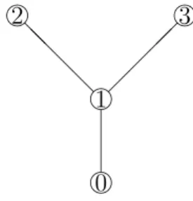
Example 2 In Figure 3 is depicted an mcst, denoted by Γ, for the mcst
situation ¯w of Figure 2. Consider τ1, τ2 ∈ ΣN such that τ1(1) = 1, τ1(2) = 2,
¡¡ ¡¡ @ @ @ @ i i i i 1 2 3 0
Figure 3: An mcst Γ for the mcst situation ¯w of Figure 2.
τ1(3) = 3 and τ2(1) = 1, τ2(2) = 3, τ2(3) = 2. Note that both τ1 and τ2 fit
with Γ but none of the other four elements of ΣN fit with Γ.
Remark 1 Let w ∈ WN0
, let Γ be an mcst for w and let τ ∈ ΣN be an order
such that Γ and τ fit. Then, X
e∈EΓ [τ (r)]0
w(e) = cw([τ (r)]) (8)
for each r ∈ {1, . . . , |N |}. So EΓ
[τ (r)]0 is an mcst for the mcst situation < [τ (r)]0, w
|[τ (r)]0 >.
Remark 2 Let w ∈ WN0
, let Γ be an mcst for w and let τ ∈ ΣN be an
order such that Γ and τ fit. The marginal vector mτ(c
w) of the mcst game
cw coincides with the Bird allocation in w corresponding to Γ and therefore
mτ(c
Remark 3 For each σ ∈ ΣEN 0 there exists a tree Γ which is an mcst for
every w ∈ Kσ; further, there exists a τ ∈ Σ
N such that Γ and τ fit.
These remarkable considerations together with the next lemma prelude to Theorem 1.
Lemma 1 Let w ∈ ¯WN0
, let Γ be an mcst for w and let τ ∈ ΣN be such
that Γ and τ fit. Let r ∈ {1, . . . , |N | − 1} and let τ0 ∈ ΣN be such that
τ0(r) = τ (r + 1), τ0(r + 1) = τ (r) and τ0(i) = τ (i) for each i ∈ {1, . . . , |N |} \
{r, r+1} (i.e. τ0 is obtained from τ by a neighbor switch of τ (r) and τ (r+1)).
Then there is an mcst Γ0 for w such that τ0 and Γ0 fit.
Proof If τ (r) is not the immediate predecessor of τ (r + 1) in Γ then take
Γ0 = Γ and then τ0 and Γ fit.
If τ (r) is the immediate predecessor of τ (r + 1) in Γ, then let k ∈ [τ (r − 1)]0
be the immediate predecessor of τ (r) in Γ. First, note that
w({k, τ (r + 1)}) ≥ w({k, τ (r)}) (9)
and
w({k, τ (r + 1)}) ≥ w({τ (r), τ (r + 1)}) (10)
because Γ is an mcst for w. Consider two cases:
c.1) w({k, τ (r)}) ≤ w({τ (r), τ (r + 1)}). Take Γ0 = (Γ \ {{τ (r), τ (r + 1)}}) ∪
{{k, τ (r + 1)}}. By inequality (9) and the isoscele triangle property
w({k, τ (r + 1)}) = w({τ (r), τ (r + 1)}) and then Γ0 is an mcst in w and
Γ0 and τ0 fit.
c.2) w({τ (r), τ (r + 1)}) < w({k, τ (r)}). Take Γ0 = (Γ \ {{k, τ (r)}}) ∪
{{k, τ (r + 1)}}. By inequality (10) and the isoscele triangle property
w({k, τ (r)}) = w({k, τ (r + 1)}) and then Γ0 is an mcst in w and Γ0 and
τ0 fit.
Theorem 1 Let w ∈ ¯WN0
.Then
ii) Let cw be the mcst game corresponding to w. Then mτ(cw) ∈ C(cw) for
all τ ∈ ΣN and cw is a concave game.
Proof
i) Let ˆΓ be an mcst for w. Then there is at least one ˆτ ∈ ΣN such
that ˆΓ and ˆτ fit. Further each τ can be obtained from ˆτ by a suitable
sequence of neighbor switches and so, by applying Lemma 1 repeatedly, we obtain the proof.
ii) Let Γ be an mcst in N0 for w and let τ ∈ Σ
N such that Γ and τ fit.
By Remark 2, it follows that mτ(c
w) coincides with the Bird allocation
corresponding to Γ. Hence, again by Remark 2, mτ(c
w) ∈ C(cw).
Fi-nally, by the Ichiishi theorem (Ichiishi (1981)) telling that a game is concave iff all marginal vectors are in the core of the game, it follows
that cw is a concave game.
Let w ∈ WN0
. We call the core of the mcst game cw¯ the Bird core of the
mcst game cw and denote it by BC(w). By Theorem 1 it directly follows that
the Bird core BC(w) of the mcst game cw is the convex hull of all the Bird
allocations corresponding to the minimum cost spanning trees for ¯w. Note
also that BC(w) ⊆ C(cw), since cw¯(S) ≤ cw(S) for each S ∈ 2N \ {∅} and
cw¯(N ) = cw(N ) (cf. Feltkamp (1995)).
Example 3 Consider the mcst situation w of Figure 1 and the corresponding
reduced mcst situation ¯w of Figure 2. Then
{1} {2} {3} {1, 2} {2, 3} {1, 3} {1, 2, 3}
cw 8 12 12 13 24 18 23
cw¯ 8 8 10 13 18 18 23
There are six minimum cost spanning trees for ¯w. Three of them lead to the
Bird allocation (8, 5, 10) and the other three to the Bird allocation (5, 8, 10).
Further, mτ(c
¯
w) = (8, 5, 10) for τ ∈ {(1, 2, 3), (1, 3, 2), (3, 1, 2)} and mτ(cw¯) =
(5, 8, 10) for τ ∈ {(2, 1, 3), (2, 3, 1), (3, 2, 1)}. The Bird core BC(w) is the
con-vex hull of the marginal vectors of the game cw¯, that is BC(w) = conv{(8, 5, 10),
(5, 8, 10)} ⊂ C(cw).
4
Monotonicity properties
In Tijs et al.(2004) a class of solutions for mcst situations which are cost monotonic is introduced: the class of obligation rules. Roughly speaking, we
define a cost monotonic solution for mcst situations as a solution such that, if the costs of some edges increase, then no agent will pay less. More precisely:
Definition 2 A solution F : WN0
→ IRN is a cost monotonic solution if for
all mcst situations w, w0 ∈ WN0
such that w(e) ≤ w0(e) for each e ∈ E
N0, it
holds that F (w) ≤ F (w0).
In this section we introduce a related concept of cost monotonicity for
mul-tisolutions on mcst situations. We call a correspondence G : WN0
³ IRN
assigning to every mcst situation w a set of cost allocations in IRN a
multi-solution.
Definition 3 A multisolution M : WN0
³ IRN is a cost monotonic
multiso-lution if for all mcst situations w, w0 ∈ WN0
such that w(e) ≤ w0(e) for each
e ∈ EN0, it holds that
M (w) ⊆ compr−(M (w0)) and M (w0) ⊆ compr+(M (w)),
where compr−(B) = {x ∈ IRN|∃b ∈ B s.t. x
i ≤ bi∀i ∈ N } and compr+(B) =
{x ∈ IRN|∃b ∈ B s.t. b
i ≤ xi ∀i ∈ N }, for each B ⊂ IRN.
Before discussing properties of the Bird core as multisolution for mcst situ-ations, we introduce the following propositions dealing with mcst situations originated by NA-semimetrics.
Proposition 3 Let w ∈ ¯WN0
and let Γ be an mcst for w and τ ∈ ΣN be
such that Γ and τ fit. Then
mτ
τ(j)(cw) = min
k∈(τ (j))0w(k, τ (j)), for each j ∈ {2, . . . , |N |}.
Proof Let j ∈ {2, . . . , |N |}. Note that by Remark 1 mττ(j)(cw) = cw([τ (j)]) − cw((τ (j))) = X e∈EΓ [τ (j)]0 w(e) − X e∈EΓ (τ (j))0 w(e). (11)
Since Γ and τ fit, we have EΓ
[τ (j)]0\ E(τ (j))Γ 0 = {{τ (j), s}}, for some s ∈ (τ (j))0.
Because EΓ
[τ (j)]0 is an mcst for w|[τ (j)]0, we have s ∈ arg mink∈(τ (j))0w({k, τ (j)}).
So X e∈EΓ [τ (j)]0 w(e) − X e∈EΓ (τ (j))0 w(e) = min k∈(τ (j))0w(k, τ (j)). (12) From (11) and (12) follows the proposition.
Proposition 4 Let w, w0 ∈ ¯WN0
be NA-semimetric mcst situations such
that w(e) ≤ w0(e) for each e ∈ E
N0. Then it holds that
mτ(cw) ≤ mτ(cw0) for each τ ∈ ΣN.
Proof Let τ ∈ ΣN. By Theorem 1 there exist two mcst’s Γ and Γ0 for w
and w0, respectively, such that they both fit with τ . First note that
mτ τ(1)(cw) = w(0, τ (1)) ≤ w0(0, τ (1)) = mττ(1)(cw0). Further mτ τ(j)(cw) = mink∈(τ (j))0w(k, τ (j)) ≤ mink∈(τ (j))0w0(k, τ (j)) = mτ τ(j)(cw0),
for each j ∈ {2, . . . , |N |}, where the first and the second equality follow by
Proposition 3 and the inequality follows from w(e) ≤ w0(e) for each e ∈ E
N0.
Theorem 2 The correspondence BC is a cost monotonic multisolution.
Proof Let w, w0 ∈ WN0
be such that w(e) ≤ w0(e) for each e ∈ E
N0. By Theorem 1 and properties of concave games, BC(w) is a convex set whose
extreme points are the marginal vectors of the game cw¯, i.e. each element
of BC(w) is a convex combination of marginal vectors of the game cw¯. Let
x ∈ BC(w). There exist numbers ατ, τ ∈ Σ
N, with 0 ≤ ατ ≤ 1 for each
τ ∈ ΣN,Pτ∈ΣNατ = 1 and x = X τ∈ΣN ατ mτ(c ¯ w). (13) Hence x = Pτ∈ΣNατ mτ(c ¯ w) ≤ Pτ∈Σ Nα τ mτ(c ¯ w0) = x0 ∈ BC(w0), (14)
where the inequality follows by Proposition 4 and the fact that ¯w(e) ≤ ¯w0(e)
for each e ∈ EN0 and the second equality by Theorem 1, which proves
BC(w) ⊆ compr−(BC(w0)). Using a similar argument the other way around
in relations (14), it follows that BC(w0) ⊆ compr+(BC(w)), which concludes
the proof.
To connect the cost monotonicity of the Bird core with cost monotonicity of obligation rules, we need Proposition 5.
Proposition 5 Let F : WN0
→ IRN be a cost monotonic and efficient
solu-tion. Then
i) F ( ¯w) = F (w) for every w ∈ WN0
;
ii) If F is also stable (i.e. F (w0) ∈ C(c
w0) for every w0 ∈ WN 0 ), then F (w) ∈ BC(w) for every w ∈ WN0 . Proof Let w ∈ WN0
. First note that by Definition 1, ¯
w(e) ≤ w(e) for each e ∈ EN0. (15)
Let Γ be an mcst for w.
i) By inequality (15) and cost monotonicity of F , F ( ¯w) ≤ F (w). On the
other hand Γ is an mcst for ¯w too and by efficiency of F
X i∈N Fi( ¯w) = X i∈N Fi(w) = w(Γ). So, F ( ¯w) = F (w). ii) By inequality (15), cw¯(S) ≤ cw(S) for all S ⊆ N, and by Definition 1 cw¯(N ) = cw(N ) = w(Γ).
Then by stability of F , F ( ¯w) ∈ C(cw¯) = BC(w) ⊆ C(cw) and by result
(i) F (w) ∈ BC(w) too.
Remark 4 Proposition 5 can be extended to multisolutions which are cost monotonic and efficient (Property 1 in next section) multisolutions. From this follows that BC is the “largest” cost monotonic stable multisolution. Remark 5 As previously said, in Tijs et al.(2004) we introduced the class of obligation rules and proved that they are both cost monotonic and stable solutions for mcst situations. So, by Proposition 5 it follows that for each
w ∈ WN0
, the set F(w) = {φ(w) | φ is an obligation rule} is a subset of the
5
An axiomatic characterization of the Bird
core
In order to introduce an axiomatic characterization of the Bird core, we need to prove the following fact for NA-semimetric mcst situations.
Lemma 2 Let w, w0 ∈ WN0
and let σ ∈ ΣEN 0 be such that w, w0 ∈ Kσ. Let
α, α0 ≥ 0. Then α ¯w, α0w¯0, αw + α0w0 ∈ Kσˆ for some ˆσ ∈ Σ EN 0.
Proof By formula (4), for each edge e ∈ EN0, there is an edge ¯e ∈ EN0 such
that ¯w(e) = w(¯e): given that e = {i, j}, ¯e is such that w(¯e) = minP∈PN 0
ij t(P ).
Note that for each w1 in the same cone Kσ as w we have ¯w1(e) = w(¯e). This
implies that for all pairs of edges e1, e2 ∈ EN0:
¯
w(e1) ≤ ¯w(e2) ⇔ w(¯e1) ≤ w( ¯e2) ⇔ ¯w1(e1) ≤ ¯w1(e2).
So, for each ¯σ ∈ ΣEN 0 we have:
¯
w ∈ K¯σ ⇔ ¯w0 ∈ Kσ¯.
Using this fact, respectively, for αw, α0w0 and αw + α0w0 ∈ Kσ in the role
of w1, we obtain: ¯ w ∈ K¯σ ⇔ α ¯w, α0w¯0, αw+ α0w0 ∈ Kσ¯ , for each ¯σ ∈ ΣEN 0. Proposition 6 Let w, w0 ∈ WN0
and let σ ∈ ΣEN 0 be such that w, w
0 ∈ Kσ.
Let α, α0 ≥ 0. Then
i) αw + α0w0 = α ¯w + α0w¯0;
ii) cαw+α0w0 = αcw¯+ α0cw¯0.
[The NA-semimetric mcst situations ¯w, ¯w0, αw+ α0w0 are obtained via
reduc-tion of the weight funcreduc-tions w, w0, αw + α0w0, respectively.]
Proof i) Note that αw + α0w0({i, j}) = min P∈PN 0 ij maxe∈E(P ) ¡ αw(e) + α0w0(e)¢ = α minP∈PN 0
ij maxe∈E(P )w(e)
+ α0min
P∈PN 0
ij maxe∈E(P )w
0(e)
where the second equality follows from the fact that w, w0and αw+α0w0
all belong to Kσ;
ii) Note that, by Lemma 2, α ¯w, α0w¯0, αw+ α0w0 ∈ Kσ¯ for some ¯σ ∈ Σ
EN 0.
For each S ∈ 2N\{∅}, there is, according to Remark 3, a common mcst
ΓS for α ¯w, α0w¯0 and αw + α0w0. Hence
αcw¯(S) + α0cw¯0(S) = P e∈ΓSα ¯w(e) + P e∈ΓSα 0w¯0(e)
= Pe∈ΓS¡α ¯w0(e) + α0w(e)¯ ¢
= Pe∈ΓS¡αw + α0w0(e)¢
= cαw+α0w0(S), where the third equality follows by (i).
Some interesting properties for multisolutions on mcst situations are the following.
Property 1 The multisolution G is efficient (EFF) if for each w ∈ WN0
and
for each x ∈ G(w) X
i∈N
xi = w(Γ),
where Γ is a minimum cost spanning network for w on N0.
Property 2 The multisolution G has the positive (POS) property if for
each w ∈ WN0
and for each x ∈ G(w)
xi ≥ 0
for each i ∈ N .
Property 3 The multisolution G has the Upper Bounded Contribution (UBC)
property if for each w ∈ WN0
and every (w, N0)-component C 6= {0}
X
i∈C\{0}
xi ≤ min
i∈C\{0}w({i, 0})
for each x ∈ G(w).
Property 4 The multisolution G has the Cone-wise Positive Linearity (CPL)
property if for each σ ∈ ΣEN 0, for each pair of mcst situations w, bw ∈ K
σ
and for each pair α, bα ≥ 0, we have
G(αw + bα bw) = αG(w) + bαG( bw).
Proposition 7 The Bird core BC satisfies the properties EFF, POS, UBC and CPL.
Proof Let w ∈ WN0
and let σ ∈ ΣEN 0 be such that w ∈ Kσ. Since
BC(w) = C(cw¯), the following considerations hold:
i) For each allocation x ∈ BC(w), Pi∈Nxi = w(Γ) for some mcst Γ by
the efficiency property of the core of the game cw¯. So BC has the EFF
property.
ii) For each allocation x ∈ BC(w), xi ≥ 0 for each i ∈ N since the Bird
core is the convex hull of all Bird allocations in the mcst ¯w, which are
vectors in IRN
+. So BC has the POS property.
iii) For each (w, N0)-component C 6= {0} and each x ∈ BC(w)
X
i∈C\{0}
xi ≤ cw¯(C \ {0}) = min
i∈C\{0}w({i, 0})
by coalitional rationality of the core of the game cw¯. So BC has the
UBC property.
iv) Let σ ∈ ΣEN 0, let w, w
0 ∈ WN0
be such that w, w0 ∈ Kσ and let
α, α0 ≥ 0. The core is in fact additive on the class of concave games
(see Dragan et al.(1989)). So,
BC(αw+α0w0) = C(cαw+α0w0) = αC(cw¯)+α0C(cw¯0) = αBC(w)+α0BC(w0). Hence BC has the CPL property.
Inspired by the axiomatic characterization of the P -value (Branzei et al.(2004)) we provide the following theorem.
Theorem 3 The Bird core BC is the largest multisolution which satisfies EFF, POS, UBC and CPL, i.e. for each multisolution F which satisfies
EFF, POS, UBC and CPL, we have F (w) ⊆ BC(w), for each w ∈ WN0
. Proof We already know by Proposition 7 that the Bird core BC satisfies the four properties EFF, POS, UBC and CPL.
Let Ψ : WN0
³ IRN be a multisolution satisfying EFF, POS, UBC and CPL.
Let w ∈ WN0
and σ ∈ ΣEN 0 be such that w ∈ K
Ψ(w) ⊆ BC(w).
First, note that by the CPL property of Ψ ³ w(σ(1))Ψ(eσ,1) + |EXN 0| k=2 ¡ w(σ(k)) − w(σ(k − 1))¢Ψ(eσ,k)´= Ψ(w). (16)
Let x ∈ ψ(w). According to (16) there exists xeσ,k
∈ Ψ(eσ,k) for each k ∈
{1, . . . , |EN0|} such that x = w(σ(1))xeσ,1 + |EXN 0| k=2 ¡ w(σ(k)) − w(σ(k − 1))¢xeσ,k .
By the UBC property, for each k ∈ {1, . . . , |EN0|} and for each (eσ,k, N0
)-component C 6= {0} we have X i∈C\{0} xeiσ,k ≤ min i∈C\{0}e σ,k ({i, 0}) = 0 if 0 ∈ C 1 if 0 /∈ C (17) implying that X i∈N xeσ,k i = X C∈C(eσ,k) X j∈C\{0} xeσ,k j ≤ |C(e σ,k)| − 1 = eσ,k(Γ),
where Γ is a minimum spanning network on N0 for mcst situation eσ,k. By
the EFF property, we have Pi∈Nxeσ,k
i = eσ,k(Γ), and then inequalities in
relation (17) are equalities, that is X i∈C\{0} xeσ,k i = 0 if 0 ∈ C 1 if 0 /∈ C. (18)
Now, consider the game ceσ,k corresponding to the simple mcst situation eσ,k.
Note that for each S ∈ 2N \ {∅},
ceσ,k(S) = |{C : C is a (e
σ,k
, N0) − component, C ∩ S 6= ∅, 0 /∈ C}|,
which is the number of (eσ,k, N0)-components not connected to 0 in eσ,k with
By (18) and the POS property, it follows that Pi∈Sxeσ,k
i ≤ ceσ,k(S) and
together with the EFF property we have xeσ,k
∈ C(ceσ,k) = BC(eσ,k).
More-over, from Proposition 6 it follows
x =³w(σ(1))xeσ,1 + |EXN 0| k=2 ¡ w(σ(k)) − w(σ(k − 1))¢xeσ,k´∈ C(c ¯ w) = BC(w). (19) Keeping into account relation (16), we have Ψ(w) ⊆ BC(w).
6
Final remarks
This paper deals mainly with the monotonicity and additivity properties of the Bird core. The attention to monotonicity properties of solutions for cost and reward sharing situations is growing in the literature.
In Sprumont (1990) attention is paid to population monotonic allocations schemes (pmas), in Branzei et al.(2001) and Voorneveld et al.(2002) to bi-monotonic allocation schemes (bi-mas) and in Branzei et al.(2002) to type monotonic allocation schemes. For mcst-situations, the existence of popula-tion monotonic allocapopula-tion schemes was established in Norde et al.(2004). For special directed mcst-situations also pmas-es exists as is shown in Moretti et al.(2002).
In Tijs et al.(2004) so called obligation rules for mcst-situations turn out to be cost monotonic and induce also a pmas. A special obligation rule is the P -value discussed in Branzei et al.(2004) (see also Feltkamp et al.(1994), Feltkamp (1995)). The P -value can be seen as a special selection of the Bird core: it corresponds to the barycenter of the Bird core (cf. Moretti et
al.(2004), Berga˜ntinos and Vidal-Puga (2004)).
For additivity properties of solutions we refer to Branzei and Tijs (2001), Tijs and Branzei (2002).
References
Aarts, H., 1994. Minimum cost spanning tree games and set games, PhD Dissertation, University of Twente, The Netherlands.
Bird, C.G., 1976. On cost allocation for a spanning tree: a game theo-retic approach, Networks 6, 335-350.
Berga˜ntinos, G., Vidal-Puga, J.J., 2004. Defining rules in cost spanning tree problems through the canonical form, EconPapers, RePEc:wpa:wuwpga: 0402004.
Branzei, R., Moretti, S., Norde, H., Tijs, S., 2004. The P -value for cost sharing in minimum cost spanning tree situations, Theory and Decision 56, 47-61.
Branzei R., Solymosi T., Tijs, S., 2002. Type monotonic allocation schemes for multi-glove games, CentER DP 2002-117, Tilburg University, The Nether-lands.
Branzei R., Tijs, S., 2001. Additivity regions for solutions in cooperative game theory, Libertas Mathematica 21, 155-167.
Branzei, R., Tijs, S., Timmer, J., 2001. Information collecting situations and bi-monotonic allocation schemes, Mathematical Methods of Operations Research 54, 303-313.
Claus, A., Kleitman, D.J., 1973. Cost allocation for a spanning tree, Net-works 3, 289-304.
Dragan, I., Potters, J., Tijs, S., 1989. Superadditivity for solutions of coali-tional games, Libertas Mathematica 9, 101-110.
Feltkamp, V., 1995. Cooperation in controlled network structures, PhD Dis-sertation, Tilburg University, The Netherlands.
Feltkamp, V., Tijs, S., Muto, S., 1994. On the irreducible core and the equal remaining obligations rule of minimum cost spanning extension prob-lems, CentER DP 106, Tilburg University, The Netherlands.
Granot, D., Claus, A., 1976. Game theory application to cost allocation for a spanning tree. Working Paper 402, Faculty of Commerce and Business Administration, University of British Columbia.
Granot, D., Huberman, G., 1981. On minimum cost spanning tree games, Mathematical Programming 21, 1-18.
greedy algorithm for LP, Journal of Economic Theory 25, 283-286.
Kruskal, J.B., 1956. On the shortest spanning subtree of a graph and the traveling salesman problem, Proceedings of the American Mathematical So-ciety 7, 48-50.
Moretti, S., Norde, H., Pham Do, K.H., Tijs, S., 2002. Connection prob-lems in mountains and monotonic allocation schemes, Top 10, 83-99.
Moretti, S., Tijs, S., Branzei, R., Norde, H., 2004. Conservative construct and charge rules for minimum cost spanning tree situations, Working Paper. Norde, H., Moretti, S., Tijs, S., 2004. Minimum cost spanning tree games and population monotonic allocation schemes, European Journal of Opera-tional Research 154, 84-97.
Prim, R.C., 1957. Shortest connection networks and some generalizations, Bell Systems Technical Journal 36, 1389-1401.
Sprumont, Y., 1990. Population monotonic allocation schemes for coop-erative games with transferable utility, Games and Economic Behavior 2, 378-394.
Tijs, S., Branzei, R., 2002. Additive stable solutions on perfect cones of cooperative games, International Journal of Game Theory 31, 469-474. Tijs, S., Branzei, R., Moretti, S., Norde, H., 2004. Obligation rules for minimum cost spanning tree situations and their monotonicity properties, CentER DP 2004-53, Tilburg University, The Netherlands.
Voorneveld, M., Tijs, S. and Grahn, S., 2002. Monotonic allocation schemes in clan games, Mathematical Methods of Operations Research 56, 439-449.