HAL Id: lirmm-01304458
https://hal-lirmm.ccsd.cnrs.fr/lirmm-01304458
Submitted on 9 Oct 2019
HAL is a multi-disciplinary open access
archive for the deposit and dissemination of
sci-entific research documents, whether they are
pub-lished or not. The documents may come from
teaching and research institutions in France or
abroad, or from public or private research centers.
L’archive ouverte pluridisciplinaire HAL, est
destinée au dépôt et à la diffusion de documents
scientifiques de niveau recherche, publiés ou non,
émanant des établissements d’enseignement et de
recherche français ou étrangers, des laboratoires
publics ou privés.
Parallel Robots Driven by n + 2 Cables
Marc Gouttefarde, Johann Lamaury, Christopher Reichert, Tobias Bruckmann
To cite this version:
Marc Gouttefarde, Johann Lamaury, Christopher Reichert, Tobias Bruckmann. A Versatile Tension
Distribution Algorithm for n-DOF Parallel Robots Driven by n + 2 Cables. IEEE Transactions on
Robotics, IEEE, 2015, 31 (6), pp.1444-1457. �10.1109/TRO.2015.2495005�. �lirmm-01304458�
A Versatile Tension Distribution Algorithm for
n
-DOF Parallel Robots Driven by
n
+ 2
Cables
Marc Gouttefarde, Johann Lamaury, Christopher Reichert, and Tobias Bruckmann
Abstract—Redundancy resolution of redundantly actuated cable-driven parallel robots (CDPRs) requires the computation of feasible and continuous cable tension distributions along a trajectory. This paper focuses on n-DOF CDPRs driven by n+2 cables since, for n = 6, these redundantly actuated CDPRs are relevant in many applications. The set of feasible cable tensions of n-DOF n+2-cable CDPRs is a two-dimensional convex polygon. An algorithm that determines the vertices of this polygon in a clockwise or counterclockwise order is first introduced. This algo-rithm is efficient and can deal with infeasibility. It is then pointed out that straightforward modifications of this algorithm allow the determination of various (optimal) cable tension distributions. A self-contained and versatile tension distribution algorithm is thereby obtained. Moreover, the worst-case maximum number of iterations of this algorithm is established. Based on this result, its computational cost is analyzed in detail, showing that the algorithm is efficient and real-time compatible even in the worst case. Finally, experiments on two 6-DOF 8-cable CDPR prototypes are reported.
I. INTRODUCTION
C
ABLE-DRIVEN parallel robots (CDPRs) consist essen-tially of a mobile platform (the end-effector) driven by cables in a parallel topology, the cable lengths being controlled by means of winches. They possess several advantages such as a potentially very large workspace. Some previous works focused on crane-like applications, e.g. [1]–[3], haptic inter-faces [4], [5], rehabilitation [6]–[8], and giant radio telescopes [9], [10].The context of this paper is the real-time control of redun-dantly actuated CDPRs intended for industrial applications. Experiments on two redundantly actuated 6 degree-of-freedom (DOF) 8-cable CDPR prototypes, CABLAR [11] (Fig. 1) and COGIRO [12], [13] (Fig. 2), will be presented. On the one hand, CABLAR is an example where actuation redundancy is required because using more cables than DOFs is a well-known necessary condition to fully constrain a CDPR mo-bile platform (wrench-closure), e.g. see [14], [15]. On the other hand, for CDPRs in a crane-like configuration [1]–[3]
Marc Gouttefarde and Johann Lamaury are with the Robotics Department, Laboratory of Informatics, Robotics and Microelectronics of Montpellier (LIRMM, CNRS-UM), 161 rue Ada, 34095 Montpellier Cedex 5, France, e-mail: [email protected].
Christopher Reichert and Tobias Bruckmann are with the Chair for Mecha-tronics, University of Duisburg-Essen, 47057 Duisburg, Germany.
The research leading to these results has received funding from the Eu-ropean Community’s Seventh Framework Programme under grant agreement No. NMP2-SL-2011-285404 (CableBOT). The financial support of the ANR (grant 2009 SEGI 018 01) and of TECNALIA are also greatly acknowledged. The authors would like to thank the German Federal Ministry of Education and Research which supports the project ”Entwicklung eines neuartigen Regalbedienger¨ates auf Basis der Stewart-Gough-Plattform” (01IC10L28A) within the ”EffizienzCluster LogistikRuhr”.
Fig. 1. CABLAR CDPR prototype. Source and Copyright c: Lehrstuhl f¨ur
Rechnereinsatz in der Konstruktion, University Duisburg-Essen.
Fig. 2. LIRMM/TECNALIA COGIROsuspended CDPR prototype.
(suspended CDPRs), actuation redundancy is not required but it can be advantageous, e.g., it allows COGIRO to have a large workspace-to-footprint ratio. This paper is dedicated to redundantly actuated CDPRs driven by n + 2 cables where n denotes the number of mobile platform DOF. Most existing redundantly actuated CDPRs are driven byn+1 or n+2 cables [11], [13], [14], [16]–[22], probably because it represents a trade-off between the benefits of actuation redundancy and the CDPR complexity and cost. For 6-DOF CDPRs, driving the platform withn + 2 = 8 cables rather than with n + 1 = 7 cables leads generally to a larger and more homogeneous workspace. It also makes the integration into a workshop or a warehouse easier since symmetric cable arrangements in a cuboid supporting frame can be used. Hence, 6-DOF CDPRs driven by eight cables are relevant in many applications. This paper focuses on redundantly actuated CDPRs but, in some
applications, CDPR driven by less than n cables, e.g. [23], may also be relevant.
The cable tension vector t ∈ Rm, m being the number of
cables, is said feasible if it satisfies 0 ≤ tmin ≤ t ≤ tmax.
The tensions have to be non-negative since the cables cannot push on the mobile platform. The maximum values tmax are
generally set by the breaking loads of mechanical parts or by the maximum actuator torques while positive values in tmin
should avoid slack cables. In the case of redundantly actuated CDPRs, infinitely many feasible cable tension distributions exist when the platform pose (position and orientation) lies inside the wrench-feasible workspace (WFW) [24], [25]. For control purposes, the resulting redundancy resolution problem must be solved in real time and the computed cable tensions must be continuous along the prescribed mobile platform trajectory.
In several previous works, optimal tension distributions are computed. The objective function can be the 1-norm [2], [18], [19], [26] or ∞-norm [27] of t but these choices are prone to cable tension discontinuities along a trajectory [26], [28]. Hence, thep-norm should rather be used with 1 < p < ∞ [29]. In particular, the 2-norm has often been selected, e.g. [30]– [34]. To compute such optimal tension distributions, iterative optimization algorithms can be used. Since the platform pose evolves continuously along a trajectory, warm start is possible which generally results in a reduced number of iterations before convergence, and thus in fast computations. Never-theless, these iterative algorithms usually have an unknown, unbounded or very large worst-case computation time which is an issue for safe real-time implementations. This issue is solved in [34], [35] where the 2-norm and barycenter tension distributions are calculated with a relatively high but bounded worst-case complexity. Besides, the methods in [36]– [39] make simple, fast and predictable computations suitable for degrees of redundancy larger than two or three. However, these methods are not proved to work in the whole WFW [38] and they may not be effective for suspended CDPRs. To enlarge the part of the WFW in which they work, some cable tensions are set at their maximum or minimum admissible values, which may be contrary to the desired behavior and degrade the smoothness of the tension time evolutions (see the example in [39]). Furthermore, a general issue is the exact nature of the computed solution which cannot be chosen, e.g., no optimality criterion can be assigned to it.
Depending on the CDPR type (suspended or fully con-strained) and on the required characteristics (e.g. high stiffness, low power consumption), the desired cable tension distribution is not always the same. For example, the minimization of energy consumption leads naturally to the 1-norm or 2-norm optimal tension distributions [2], [18], [19], [30]–[32] whereas the methods presented in [22], [26], [35] can be used to increase stiffness since they avoid low cable tensions. Therefore, a versatile method which can compute several types of cable tension distributions is of great interest. Moreover, the method should be mostly based on a single algorithm as independent as possible from specialized computational libraries (e.g. optimization algorithms) in order to avoid im-plementing or linking several different algorithms in a
real-time control software environment. Additionally, a “safe” and reliable implementation requires a proved and real-time compatible worst-case computation time.
In most of the previously cited works, one type of tension distribution is computed. Exceptions are [22], [26] where parameters can be used to steer the cable tensions toward lower or higher values. However, such parameters may have a little effect as reported in [26] and the selection of their values may be an issue. Notably, they cannot be used to compute a prescribed tension distribution type (e.g. the 2-norm optimal distribution). Moreover, the method presented in [26] relies on a LP formulation so that discontinuities may occur and its worst-case complexity has not been established. In [22], the management of infeasibility is an issue and the use of an iterative optimization algorithm precludes a worst case complexity analysis. In [19], several tension distributions are computed but only low cable tension values are of interest, the computations mostly rely on optimization routines, and only planar CDPRs are considered. The method introduced in [39] could lead to versatile tension distribution computations but it has the drawbacks already pointed out above.
The present paper introduces a versatile tension distribution algorithm dedicated ton-DOF CDPRs driven by n + 2 cables. For a given pose of the mobile platform of these CDPRs, the set of feasible cable tensions is known to be a convex polygon (Section II). The main contribution is an efficient geometric algorithm which either determines in order the vertices of this polygon or prove that it is empty (Section III). Moreover, the algorithm starting point is not required to correspond to a feasible cable tension vector. Another contribution is to point out that various (optimal) cable tension distributions can be obtained by straightforward uses or modifications of this algorithm (Section IV). Specifically, the determinations of the optimal 1-norm and 2-norm as well as the centroid and weighted barycenter tension distributions are explained. The worst-case maximum number of iterations of the algorithm is then established and its computational cost is analyzed (Section V). It is thereby proved to be efficient and well suited to real-time implementations. Its computational effi-ciency is also briefly compared to some previous methods. Finally, experimental results obtained on two 6-DOF 8-cable prototypes, the fully-constrained CDPR CABLAR and the suspended CDPR COGIRO, are presented (Section VI).
In the preliminary versions [13], [40] of the method intro-duced in this paper, the algorithm was not capable of dealing with infeasibility, its computational cost was not established, only the centroid cable tension distribution was computed, and experiments were conducted only on the COGIRO CDPR.
II. FEASIBLECABLETENSIONPOLYGON
Then × m wrench matrix W maps the cable tension vector t∈ Rmto the wrench f∈ Rn applied by the cables onto the
mobile platform, e.g. [14], [15]
Wt= f (1)
where m and n denote the number of cables and of mobile platform DOF, respectively. Let r = m − n be the degree of
−5 0 5 −5 0 5 0 5 x(m) 8 7 1 R0 x0 2 z0 y(m) 6 y0 5 3 4 z(m)
(a) Schematic view
−5000 0 5000 −5000 −4000 −3000 −2000 −1000 0 1000 2000 3000 4000 5000 λ1 λ 2 (b) Feasible polygonA−1(Λ)
Fig. 3. The COGIRO suspended CDPR in static equilibrium at pose [1 3 2.5 15 35 25]T(units: meters and degrees, XYZ Euler angle convention)
with a300 kg platform mass, tmin= 100 N and tmax= 5000 N.
actuation redundancy (DOR). This paper is dedicated to the caser = 2 DOR. When W has full rank, Eq. (1) is equivalent to the following well-known equation
t= W+f+ Nλ (2)
where W+ is the Moore-Penrose pseudoinverse of the wrench matrix, N = null(W) is a full rank m × 2 matrix and λ = [λ1 λ2]T is an arbitrary2-dimensional vector. The two
columns of N form an orthonormal basis of the2-dimensional nullspace of W, i.e., NTN= I2. tp = W+f is the
minimum-norm solution of (1) satisfying tT
pN = 0 and Nλ is the
homogeneous solution where N maps λ into the nullspace of W. Let Σ ⊂ Rm be the 2-dimensional affine space of the
solutions to (1) and Ω ⊂ Rm the m-dimensional hypercube
of feasible cable tensions, i.e., Σ = {t | Wt = f}
Ω = {t | ti∈ [tmin, tmax] , 1 ≤ i ≤ m}.
(3) The intersectionΛ = Ω∩Σ is a 2-dimensional convex polytope representing the set of feasible cable tension distributions, e.g. [15], [28], [33]. Under the affine map A = (N, tp), the
preimage of Λ is also a 2-dimensional convex polytope, i.e., a convex polygon, defined as
A−1(Λ) = {λ ∈ R2| tmin ≤ tp+ Nλ ≤ tmax}. (4)
In the sequel,A−1(Λ) is refer to as the feasible polygon. For
example, Fig. 3 shows the feasible polygon corresponding to a particular platform pose of a 6-DOF 8-cable suspended CDPR. In fact, the feasible polygon A−1(Λ) is defined by the
following set of 2m linear inequalities
tmin− tp≤ Nλ ≤ tmax− tp (5)
where each inequality defines a half-plane bounded by a line corresponding to values of λ for which one cable tension is equal to tmin ortmax. The intersection of the 2m half-planes
in (5) forms the feasible polygonA−1(Λ).
The feasible polygonA−1(Λ) has been considered only in
a few previous works [19], [35]. It lies in the 2-dimensional space of vectors λ as opposed to Λ which is embedded into the m-dimensional space of cable tensions (in this paper, m = 8 for n = 6 DOF). Hence, the consideration of
A−1(Λ) allows to work in a 2-dimensional space where simple
geometric reasoning can be made. In fact, Section III shows how polygon edges can be followed to reach a feasible point (if it exists) and then to compute all the feasible polygon vertices in order. The knowledge of the vertices (in a clockwise or counterclockwise order) completely determines the polygon geometry and thus allows a direct determination of various tension distributions (Section IV). The idea of following the polygon edges to compute its vertices is simple but, to the best of our knowledge, has never been used—at least in the context of CDPR cable tension distribution computation.
Note that, as pointed out in [19], [35], the vertices of A−1(Λ) can be merely computed by solving all the 2 × 2
linear systems obtained by setting two of the inequalities in (5) to equalities. Each such system provides one vector λ which is an actual vertex of the polygonA−1(Λ) if it verifies
all the inequalities in (5). There are 2m inequalities in (5) and, when inequalities are set to equalities, each row of (5) defines two parallel straight lines. Hence, the total number of 2 × 2 linear systems to be solved is C2m
2 − m = 4C2m
[26] (112 in the case m = 8). This brute-force determination is simple but time-consuming. Moreover, the geometry of A−1(Λ) is not fully revealed until the vertices are arranged in a
clockwise or counterclockwise order. Hence, this brute-force determination must generally be followed by a convex hull and/or a triangulation algorithm [35] which further increases its computational cost. Section III will show that the vertices of A−1(Λ) can be more efficiently computed in the case
m = n + 2.
III. EFFICIENTDETERMINATION OF THEFEASIBLE
POLYGONVERTICES
This section introduces the main contribution of this paper: An efficient algorithm which either determines the vertices of the feasible polygon or proves that the system of linear inequalities (5) is unfeasible. The algorithm can start at any intersection point (feasible or not) between two lines bounding half-planes defined by inequalities of (5). Moreover, the ver-tices are determined in a clockwise or counterclockwise order which allows a direct determination of various cable tension distributions (as discussed in Section IV).
A. Notations
Prior to the detailed description of the proposed algorithm, this section first introduces some notations.
The system of linear inequalities (5) is composed of m rows. Its row i ∈ {1, . . . , m} consists of two inequalities: tmin − tpi ≤ niλ and niλ ≤ tmax− tpi, where the two-dimensional row vector ni denotes the row i of N. Each of
these 2m inequalities defines a half-plane. In the sequel, the straight line bounding this half-plane is called an inequality
line and the point of intersection between two of these inequality lines is referred to as an intersection point. Note that the two lines bounding the two half-planes defined by one row of (5) are parallel.
A row of (5) is said to be satisfied at a point λ if the two inequalities of this row are satisfied. A point is said to
be feasible if all the rows of (5) are satisfied at this point, otherwise it is unfeasible. The feasible index set at a given point λ is the set consisting of the indices of the rows of (5) satisfied at λ, e.g., if rows 2, 4, 5 and 7 are satisfied, the corresponding feasible index set isI = {2, 4, 5, 7}. Moreover, the feasible polygonPIassociated to a given feasible index set
I is the set of points λ at which all the rows of (5) with indices in I are satisfied. PI is the intersection of the half-planes
defined by the inequalities of these rows of (5). The edges and vertices ofPIare segments of inequality lines and intersection
points, respectively. ForI = {1, . . . , m}, the feasible polygon associated toI is P{1,...,m}= A−1(Λ). The feasible index set
associated to a feasible point is I = {1, . . . , m}.
B. Algorithm General Description
The main idea is to move along the inequality lines stopping at each intersection point encountered along the way. Each move from one intersection point to the next one must either keep the current feasible index set unchanged or, as often as possible, add one or several rows of (5) to this set. In other words,I being the feasible index set at some intersection point v, a move along an inequality line to another intersection point v′is made only if the feasible index setI′at v′is such thatI ⊆
I′. The number of rows of (5) which are satisfied at the current
intersection point is thus equal to or greater than the number of rows satisfied at all the previously visited intersection points. In this way, the algorithm aims at reaching the feasible polygon A−1(Λ), if it exists, and then at turning around it. In order
not to retrace its steps, if the current intersection point v has been reached by following the inequality line Li, the other
inequality line intersecting Li at v is followed in order to
move to the next intersection point v′.
Since there is a finite number of intersection points—a maximum of4Cm
2 , see Section II,— the algorithm eventually
reaches an intersection point which has already been visited before. Let vfdenote this intersection point,Ifbe the feasible
index set at vf andPIf the feasible polygon associated toIf. The intersection point vf is a vertex ofPIf and the algorithm is terminated at vf. Indeed, as demonstrated in Section III-D,
a full turn around PIf has been made to go back to vf, i.e., all the vertices of PIf were visited in a clockwise or counterclockwise order. If the algorithm were not stopped, the same full turn aroundPIf would be made again and again.
Furthermore, only two cases are possible when the algo-rithm terminates at vf.
• Case 1: vf is feasible, i.e., all the inequalities of (5)
are satisfied at this point, If = {1, . . . , m} and PIf = A−1(Λ). In this first case, all the vertices of A−1(Λ)
have been visited and thus determined in a clockwise or counterclockwise order since the algorithm made a full turn aroundA−1(Λ).
• Case 2: vf is not feasible, If 6= {1, . . . , m} and PIf 6=
A−1(Λ). In this second case, the inequality system (5) is
proved to be unfeasible, i.e., A−1(Λ) = ∅. Otherwise, as
demonstrated in Section III-D, the algorithm would have reached a vertex of A−1(Λ).
Last but not least, because feasibility is not required to start
the algorithm, the initial point vinitwhere the algorithm begins
moving along the inequality lines can be the intersection point between any two inequality lines of (5).
C. Next Intersection Point
The determination of the next intersection point to be reached is the main part of the algorithm. It is repeatedly executed until the algorithm terminates.
Let us consider that the algorithm already reached point vij
which is the intersection between the two inequality linesLi
andLj. Indexi (resp. j) designates the row of (5) containing
the inequality which defines the halfplane bounded by Li
(resp. Lj). vij is not necessarily feasible and the feasible
index set at vij is denoted Iij. Let us also consider that the
algorithm reached vij by moving along Lj. Hence, line Li
must be followed in order to move to the next intersection point. The latter will be the first intersection point encountered alongLi while moving from vij in the direction which keeps
the inequality corresponding to Lj satisfied. This inequality
must be kept satisfied because index j is not authorized to leave the current feasible index setIij.
First, let us determine the appropriate “direction of motion”. Line Li is to be followed and the row ni of N is a vector
orthogonal to Li. Therefore, the appropriate direction of
motion is a vector orthogonal to ni. Let this vector be the
row vector ni⊥: nin T
i⊥ = 0. The points λ belonging to Li are given by
λ= vij+ αnTi⊥ (6)
whereα is a scalar. Let us choose α ≥ 0 as the appropriate direction of motion along Li. With the notation ni = [a b],
ni⊥ can be equal to one of the following two vectors: ni⊥1 = [b − a] or ni⊥2 = [−b a]. Between ni⊥1and ni⊥2, the appropriate choice for ni⊥ is the one such that the inequality corresponding to Lj remains satisfied for points λ given by
(6). Then, njλ= bj− tpj being the equation ofLj, it is not difficult to prove that [40]:
• If bj = tmin, among ni⊥1 and ni⊥2, the appropriate choice for ni⊥ is the one such that njn
T i⊥ ≥ 0.
• If bj = tmax, the appropriate choice for ni⊥ is the one such that njnTi⊥ ≤ 0.
The appropriate direction of motion ni⊥ being known, the length of the move along Li, i.e. the value of α in (6),
which allows the algorithm to reach the next intersection point vlimust now be determined. This next intersection point
corresponds to the smallest α ≥ 0 such that one of the inequalities of (5), apart from the two inequalities of row i, becomes an equality. Therefore, let us consider rowk of (5)
tmin− tpk ≤ nkλ≤ tmax− tpk, k ∈ {1, . . . , m}\{i} (7) where λ is given by (6). Let Lk,min and Lk,max be the
inequality lines corresponding to the left-hand side and right-hand side inequalities of (7), respectively. The following cases have to be distinguished.
1. nknTi⊥ = 0: The two inequality lines Lk,min and Lk,max are parallel toLiand no intersection point betweenLiand
these two lines can be found. 2. nknTi⊥ > 0:
a. If nkvij≤ tmin− tpk, the intersection point betweenLi and Lk,min is obtained for α = αk = (tmin − tpk− nkvij)/(nknTi⊥) ≥ 0. Li also intersects Lk,max but for a larger value ofα.
b. Iftmin− tpk< nkvij ≤ tmax− tpk, the intersection point between Li and Lk,max is obtained for αk = (tmax−
tpk−nkvij)/(nkn T
i⊥) ≥ 0. Lialso intersectsLk,minbut for a negative value ofα.
c. Iftmax− tpk< nkvij, there is no intersection λ between Li andLk,min orLk,max such that α ≥ 0 in (6).
3. nknTi⊥ < 0:
a. If nkvij < tmin − tpk, there is no intersection point betweenLi andLk,min orLk,max such that α ≥ 0.
b. Iftmin− tpk≤ nkvij < tmax− tpk,αk = (tmin− tpk− nkvij)/(nknTi⊥) is the nonnegative value of α such that Li intersectsLk,min.Li also intersects Lk,max but for
a negative value ofα.
c. If tmax− tpk ≤ nkvij, the intersection point between Li and Lk,max is obtained for αk = (tmax − tpk − nkvij)/(nknTi⊥) ≥ 0. It is smaller than the value of α for whichLi intersectsLk,min.
At mostm−1 nonnegative scalars αkare thereby computed.
The smallest one
αl= min
k αk (8)
determines the next intersection point vli where l =
argmink(αk). The inequality line Ll which intersects Li at
vli is eitherLl,minorLl,max depending on the sign of nlnTi⊥ and on the value of nlvij as detailed above.
The feasible index set Ili at vli is such that Ili ⊇ Iij.
In fact, two cases should be distinguished. First, if l 6∈ Iij,
Ili= Iij∪ {l} since row l of (5) is now satisfied (cases 2.a
and 3.c) while all the rows of (5) with indices in Iij remain
satisfied because αl has been chosen as the smallest αk. A
new feasible polygonPIli has been reached and vliis its first visited vertex. Second, if l ∈ Iij, we have Ili = Iij (cases
2.b and 3.b above). The algorithm kept on turning around the current feasible polygonPIij = PIli and:
• If vliis not the first visited vertex ofPIij, the algorithm will keep on turning around this feasible polygon by looking for the next intersection point.
• Otherwise, the algorithm is back at the first visited vertex
of the current feasible polygonPIij = PIli. A full turn around this polygon has been made and the algorithm is terminated. IfIli= {1, . . . , m}, the inequality system (5)
is feasible, the current feasible polygon isA−1(Λ) and all
the vertices ofA−1(Λ) have been determined. Otherwise,
Ili ⊂ {1, . . . , m} (strict inclusion) and the inequality
system (5) is proved to be unfeasible (A−1(Λ) = ∅).
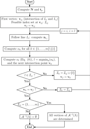
The flowchart of Fig. 4 summarizes the main steps of the algorithm introduced in this section.
D. Termination and Proofs
The algorithm presented in Sections III-B and III-C always goes back to an already visited intersection point, denoted vf,
because there is a finite total number of intersection points (a maximum of 4Cm
2 ). The proof below shows that, on the way
End Start Yes Yes No No Yes No Compute N and tp vf= vli Ili= Iij∪ {l} j= i, i = l
Compute αkfor all k ∈ {1, . . . , m}\{i}
A−1(Λ) = ∅
are determined All vertices of A−1(Λ)
Follow line Li: compute ni⊥
First vertex: vij(intersection of Liand Lj)
Feasible index set at vij: Iij
vf= vij
Compute αl(Eq. (8)), l = argmink(αk),
and the next intersection point vli
vli= vf? l∈ Iij?
Iij= {1, . . . , m} ?
Ili= Iij
Fig. 4. Flowchart of the algorithm of Section III.
back to vf, all the vertices of the feasible polygonPIf are visited, where If denotes the feasible index set at vf.
Proof 1. When the algorithm first reaches vf, it begins to turn
around the convex polygon PIf, visiting the vertices of PIf in a clockwise or counterclockwise order. Hence, assuming that one vertex of PIf is not visited amounts to assume that a move from some vertex of PIf led the algorithm to visit an intersection point v which is not a vertex of PIf. By construction of the algorithm (Section III-C), the feasible index set I at v satisfies If ⊆ I since vf was visited before v.
In fact, since v is not a vertex of PIf, we have If ⊂ I, i.e.,If is a proper (strict) subset ofI. However, after having
visited v, the algorithm goes back to vf so that, according to
Section III-C, I ⊆ If. This is a contradiction since we have
If ⊂ I and I ⊆ If. Hence, v cannot be visited which proves
that all the vertices of PIf are necessarily visited since the algorithm cannot take another path on its way back to vf.
This proof also demonstrates that if the algorithm were not stopped at vf, the same full turn around PIf would be made repeatedly. Therefore, the algorithm is stopped at vf and two cases are possible. First, if If = {1, . . . , m},
PIf = A
−1(Λ), the inequality system (5) is feasible and all
the vertices ofA−1(Λ) have been determined in order. Second,
if If 6= {1, . . . , m}, i.e. If ⊂ {1, . . . , m}, let us prove that
the inequality system (5) is unfeasible, i.e., A−1(Λ) = ∅.
Proof 2. Assume, to the contrary, that A−1(Λ) is not the
empty set. SinceA−1(Λ) = P
{1,...,m} andIf ⊂ {1, . . . , m},
A−1(Λ) is included into P
of {1, . . . , m} (If ⊂ {1, . . . , m}), there is k ∈ {1, . . . , m}
such that k 6∈ If. One of the two inequality lines associated
to row k of (5), denoted Lk, is thus supporting an edge of
A−1(Λ) while cutting P
If in two parts. Consequently, Lk intersects two edges of PIf and the feasible index set at the two corresponding intersection points is If∪ {k}. Since
If∪ {k} is larger than If, the algorithm necessarily stops at
one of these two intersection points while turning aroundPIf. From this point on, it leaves the boundary ofPIf by following Lk to the interior of PIf. It means that an intersection point v which is not a vertex of PIf will be visited which is impossible according to Proof 1 above. Necessarily, we have A−1(Λ) = ∅.
E. Degenerate Cases
Degeneracy may happen when inequality lines correspond-ing to different rows of (5) are parallel or when three or more of these lines have a common intersection point.
The first degenerate case corresponds to Case 1. of Sec-tion III-C (nknTi⊥ = 0) and is not difficult to handle. The second one, three or more inequality lines intersecting at a given point, corresponds to the particular case αl= 0 in (8).
Equivalently, with the notations of Section III-C, there exists k ∈ {1, . . . , m}\{i} such that αk = 0. It means that the
three lines Li, Lj and Lk (where Lk is Lk,min or Lk,max)
are crossing at vij. However, together with Lj (which was
followed to reach vij), only one ofLiorLk is supporting the
current feasible polygon PIij along one of its edges. This supporting line is to be followed to reach the next vertex of the current feasible polygon. It can be determined by straightforward geometric reasoning on the vectors ni, nj and
nk[40]. The other line intersecting at vijsupports the polygon
at a vertex only. Removing its index from consideration in (8) yields a strictly positive value of αl, i.e., it leads to the next
polygon vertex.
F. Example
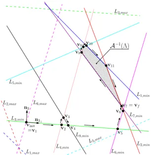
The determination of the vertices of A−1(Λ) in the case
of Fig. 3 is taken as an example. As shown in Fig. 5, the problem is feasible and the vertices v7, v8, v9, v10,
and v11 of A−1(Λ) are determined in a clockwise order.
The initial intersection point vinit has been selected as the
intersection between the inequality lines L3,min andL6,max.
This initial point is not feasible since its feasible index set is Iinit = {1, 2, 3, 5, 6}. The feasible index set at v2 is
I2 = {1, 2, 3, 4, 5, 6} whereas the feasible index set at v3,
v4, v5, and v6 is I3= {1, 2, 3, 4, 5, 6, 8}. By construction of
the algorithm, we have Iinit⊂ I2⊂ I3⊂ {1, . . . , 8}.
IV. OPTIMAL TENSION DISTRIBUTIONS
This section shows that various cable tension distributions can be obtained by a straightforward use or modification of the algorithm introduced in Section III. The determinations of the optimal 2-norm and 1-norm as well as the centroid and weighted barycenter tension distributions are explained. In the sequel, the feasible polygon A−1(Λ) is assumed to be
non-empty since, otherwise, no feasible tension distribution exists.
00000000 00000000 00000000 00000000 00000000 00000000 00000000 00000000 00000000 00000000 00000000 00000000 00000000 00000000 00000000 00000000 00000000 00000000 00000000 00000000 00000000 00000000 11111111 11111111 11111111 11111111 11111111 11111111 11111111 11111111 11111111 11111111 11111111 11111111 11111111 11111111 11111111 11111111 11111111 11111111 11111111 11111111 11111111 11111111 v3 v11 v5 v8 v4 v7= vf L3,max L5,min L6,min L2,min L4,min L6,max vinit L1,min L5,max L7,min L8,min n3 ⊥ n3 =v1 v2 L1,max L2,max L3,min v9 v6 v10 A−1(Λ)
Fig. 5. Algorithm of Section III applied to the case of Fig. 3. From the initial intersection point vinit, as indicated by the arrows, the algorithm reaches in
order the intersection points v2, . . . , v11. It finally terminates at v7 = vf
since this point was already visited before.
A. 2-norm Optimal Solution
The 2-norm optimal tension distribution is the solution of the quadratic program (QP)
min
t ktk 2
s.t. Wt = f, tmin≤ t ≤ tmax.
(9) Using Eq. (2), the objective function can be written asktk2= ktpk2+ kNλk2+ 2tTpNλ, i.e., ktk
2
= ktpk2+ kλk2 since
NTN= I2 and tTpN= 0.
For a given pose of the mobile platform, tpis a constant. The
problem can thus be reformulated in the following equivalent form min λ kλk 2 s.t. tmin− tp≤ Nλ ≤ tmax− tp. (10) This strictly convex QP has a unique global solution. When 0∈ A−1(Λ), λ = 0 is the solution of (10) and t
p = W+f is
then the optimal solution of (9). When 06∈ A−1(Λ), the
opti-mal solution of (10) lies on an edge or at a vertex ofA−1(Λ)
as illustrated in Fig. 6. The following straightforward modifi-cation of the algorithm introduced in Section III allows the determination of this solution. While turning aroundA−1(Λ),
the current vertex vij and the edge that will be followed to
reach the next vertex vliare tested for optimality. If this vertex
or a point on this edge is found to be the optimal solution λ∗2of
(10), the desired 2-norm optimal tension distribution (solution of (9)) is computed as t∗2= tp+ Nλ∗2.
By means of the Karush-Kuhn-Tucker (KKT) conditions [41], a vertex vij ofA−1(Λ) can be proved to be the solution
of (10) if and only if the two components of the vector µ= [ai, aj]−1vij (11)
are non-negative. Vertex vijis the intersection between the two
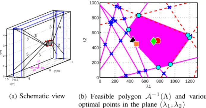
Fig. 6. A case where the solution of (10) lies on an edge ofA−1(Λ). −0.5 0 0.5 −5 0 5 0 1 2 3 4 4 2 y(m) 1 3 R0 6 z0 8 y0 x0 7 5 x(m) z(m)
(a) Schematic view
0 200 400 600 800 1000 1200 0 200 400 600 800 1000 λ1 λ 2
(b) Feasible polygon A−1(Λ) and various
optimal points in the plane(λ1, λ2)
Fig. 7. The CABLAR fully constrained CDPR in static equilibrium at pose [0 −2.5 2 3 5 0]T (units: meters and degrees, XYZ Euler angle
convention) with a 45 kg platform mass, tmin = 100 N and tmax = 600 N.
The markers indicate polygon vertices and different optimal solutions to the tension distribution problem.
and njλ= bj− tpj, respectively. In (11), ai = sin T i where
si = 1 if bi= tminandsi= −1 if bi= tmax, and aj= sjnTj
wheresj = 1 if bj= tmin andsj= −1 if bj= tmax.
Let us now consider an edge of A−1(Λ) supported by the
inequality line niλ = bi− tpi. The KKT conditions can be used to prove that the solution of (10) lies on this edge if and only if: 1. µi = si(bi− tpi)/a
T
iai ≥ 0, and 2. λ = µiai
verifies all the inequalities in (5), wheresi and ai are defined
as above. If these two conditions are true, the point λ= µiai
lies on the edge of A−1(Λ) and is the optimal solution of
(10): λ∗2 = µiai. Geometrically, this point is the orthogonal
projection of the origin λ = 0 onto the line supporting the edge.
Fig. 7 illustrates different optimal solutions obtained for the CABLAR fully constrained CDPR. The square marker represents λ∗2 which lies on a edge ofA−1(Λ).
B. 1-norm Optimal Solution
The 1-norm optimal tension distribution is the solution of the linear program
min
t 1
Tt
s.t. Wt= f, tmin≤ t ≤ tmax
(12) where 1 is the vector of Rmwhose components are all equal to 1. Eq. (2) allows (12) to be written in the equivalent form
min λ 1 T Nλ s.t. tmin− tp≤ Nλ ≤ tmax− tp. (13) since 1Tt= 1Tt
p+1TNλ. The solution of (13) lies at a vertex
ofA−1(Λ). However, some orientations of A−1(Λ) make the
1-norm minimized over an entire edge [41] and the solution is then non-unique. The use of the 1-norm optimal tension distribution is thus an issue because it may be discontinuous along a platform trajectory [26], [28], which might yield vibrations and lead to control issues.
Nevertheless, if the solution of (13) is to be computed, the algorithm introduced in Section III can be directly used since it suffices to test each visited vertex ofA−1(Λ) for optimality.
Let vijbe a vertex ofA−1(Λ) lying at the intersection between
Li and Lj whose equations are niλ = bi− tpi and njλ = bj − tpj, respectively. The KKT conditions imply that vij is the optimal solution of (13) if and only if the vector
µ= [ai, aj]−1NT1 (14)
has non-negative components. In (14), ai and aj are defined
as in Section IV-A. If vij is found be the solution of (13),
the 1-norm optimal tension distribution (solution of (12)) is calculated as t∗1 = tp + Nvij. In Fig. 7b, the 1-norm
minimum tension distribution is indicated by the triangular marker which, as expected, is located at a vertex ofA−1(Λ).
C. Centroid
The determination of the centroid λ∗c of A−1(Λ) can be
relevant for suspended CDPRs since the corresponding tension distribution is far from the boundaries ofΛ. In fact, according to [42], [43], the centroid is as far as possible from the polygon boundaries and is the unique point ofA−1(Λ) that solves
max
p log
Y
di (15)
where di is the Euclidean distance from point p to the ith
inequality line. Eq. (15) shows that the centroid depends smoothly on the problem constraints so that the corresponding tension distribution is continuous along a platform trajectory.
Let vi = [vi1 vi2]
T, i ∈ {1, . . . , q}, be the q vertices of
A−1(Λ) computed by means of the algorithm of Section III.
Since these vertices have been determined in a clockwise or counter-clockwise order, the centroid λ∗c = [λc1 λc2]
T
of A−1(Λ) is directly given by the following well-known
formulas λc1 = 1 6A q−1 P i=1
(vi1+ v(i+1)1)(vi1v(i+1)2− v(i+1)1vi2) λc2 = 1 6A q−1 P i=1
(vi2+ v(i+1)2)(vi1v(i+1)2− v(i+1)1vi2) (16) whereA is the area of the polygon, given by
A = 1 2 q−1 X i=1 (vi1v(i+1)2− v(i+1)1vi2). (17)
In Fig. 7b, the red dot marker shows λ∗c. The desired tension
D. Weighted Barycenter
All the vertices of A−1(Λ) being determined by the
al-gorithm of Section III, the weighted barycenter is another tension distribution that can be directly computed. In order to avoid discontinuities that may be created when the same weight value is used for all vertices [44], each vertex vi can
be weighted by wi= 2 X j=1 kvi− vijk /kvik (18)
where vi1 and vi2 are the two neighbor vertices of vi. The
weighted barycenter ofA−1(Λ) is then computed as
λw= q X i=1 wivi ! , q X i=1 wi (19)
and the desired tension distribution is tw= tp+ Nλw. This
solution is shown in Fig. 7b by the diamond marker. V. COMPUTATIONALEFFICIENCY
In this section, the maximum number of moves (iterations) made by the algorithm of Section III is determined. Based on this result, a detailed analysis of the number of operations required by the proposed tension distribution algorithm is presented together with brief comparisons to some previously proposed methods.
A. Number of Feasible Polygon Vertices
By geometric reasoning, let us prove that the number of verticesnvof a feasible polygonPIsatisfiesnv≤ 2|I|, where
|I| is the number of elements of I. This result will be used in Section V-B.
In the case|I| = 2, two pairs of parallel inequality lines are intersecting as shown in Fig. 8a. Without loss of generality, let the first pair be L1,min, L1,max (row 1 of (5)) and the
second pair be L2,min, L2,max (row 2 of (5)). The resulting
feasible polygonPI=2is a parallelogram so thatnv= 4 when
|I| = 2. In the case |I| = 3, a third pair of parallel inequality lines L3,min and L3,max (row 3 of (5)) is added as shown
in Fig. 8b. The corresponding feasible polygonPI=3 has the
maximum possible number of vertices when bothL3,minand
L3,max cut one and only one vertex out of PI=2. Indeed, as
illustrated in Fig. 8b, an additional inequality line creates new vertices by cutting some vertices out of the current polygon. The polygon being convex, at most two vertices can be created and at least one vertex is cut out in the process, i.e., at most one vertex is added.L3,minandL3,maxadd thus at most 2 vertices
to the previous 4-vertex polygonPI=2so thatnv ≤ 6 holds
for|I| = 3. By induction on the number of pairs of inequality lines definingPI, the same reasoning leads tonv≤ 2|I|.
B. Maximum Total Number of Moves
Let vinit be the intersection point where the algorithm
introduced in Section III starts. The feasible index set at vinit
is denoted Iinit. On its way to the last intersection point vf,
the algorithm considers a sequence of feasible index setsI(i).
000000000000000000000000 000000000000000000000000 000000000000000000000000 000000000000000000000000 000000000000000000000000 000000000000000000000000 000000000000000000000000 000000000000000000000000 000000000000000000000000 000000000000000000000000 000000000000000000000000 000000000000000000000000 000000000000000000000000 000000000000000000000000 111111111111111111111111 111111111111111111111111 111111111111111111111111 111111111111111111111111 111111111111111111111111 111111111111111111111111 111111111111111111111111 111111111111111111111111 111111111111111111111111 111111111111111111111111 111111111111111111111111 111111111111111111111111 111111111111111111111111 111111111111111111111111 L2,max L2,min L1,min L1,max PI=2 (a)|I| = 2 000000000000000000 000000000000000000 000000000000000000 000000000000000000 000000000000000000 000000000000000000 000000000000000000 000000000000000000 000000000000000000 000000000000000000 000000000000000000 000000000000000000 000000000000000000 000000000000000000 111111111111111111 111111111111111111 111111111111111111 111111111111111111 111111111111111111 111111111111111111 111111111111111111 111111111111111111 111111111111111111 111111111111111111 111111111111111111 111111111111111111 111111111111111111 111111111111111111 L2,max L2,min L1,min L1,max L3,min cut vertex L3,max PI=3 (b)|I| = 3 Fig. 8. Feasible polygonsPI with|I| = 2 (left) and |I| = 3 (right).
Without loss of generality (reordering if necessary), let the first index set beIinit= I(1) = {1, . . . , p} where p is the number
of rows of (5) satisfied at vinit (p ≤ m). If (5) is feasible, the
(last) feasible index set at vf isIf = {1, . . . , m}, otherwise it
isIf ⊂ {1, . . . , m}. The maximum number of feasible index
sets in the sequence is thus obtained when (5) is feasible in which case If = I(m − p + 1) = {1, . . . , m}. The ith
index set in the sequence isI(i) = {1, . . . , p, . . . , p + i − 1}, 1 ≤ i ≤ m−p+1. The number of vertices of the corresponding feasible polygon PI(i) is denoted nv(i). When I(i) is the
current feasible index set, the algorithm “moves” along the edges ofPI(i)from one vertex to the next one. Letnm(i) be
defined as the number of moves along the edges ofPI(i)such
thatI(i) is the feasible index set of the vertices from where the moves are made (1 ≤ nm(i) ≤ nv(i)).
The maximum total number of moves (iterations) made by the algorithm of Section III is equal to
nmt= m−p+1
X
i=1
nm(i). (20)
An upper bound onnmt, depending only onp and m, can be
established by analyzing the relationship between the number of verticesnv(i + 1) of PI(i+1), the number of verticesnv(i)
of PI(i), and the number of moves nm(i) along the edges
of PI(i). First, since I(i + 1) = I(i) ∪ {p + i}, PI(i+1)
is obtained from PI(i) by cutting it with the two inequality
lines Lp+i,min and Lp+i,max which correspond to the row
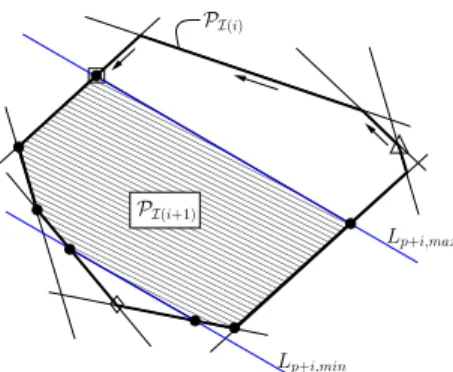
p + i of (5), as illustrated in the example shown in Fig. 9. Second, by definition of nm(i), the algorithm of Section III
stops atnm(i) vertices of PI(i)before meeting one of the two
inequality linesLp+i,min orLp+i,max, i.e., before reaching a
vertex ofPI(i+1). Therefore, the inequality lineLp+i,min or
Lp+i,maxon which this vertex lies (Lp+i,maxin Fig. 9) cuts at
leastnm(i) vertices of PI(i)while creating two new vertices.
The other inequality line (Lp+i,minin Fig. 9) cuts at least one
vertex of PI(i) while creating two new vertices. Hence, the
number of vertices ofPI(i)which are also vertices ofPI(i+1)
is at most equal tonv(i)−nm(i)−1 and the number of vertices
created by Lp+i,min andLp+i,max is at most equal to four.
The number of verticesnv(i + 1) of PI(i+1) is thus bounded
as follows
0000000000000000 0000000000000000 0000000000000000 0000000000000000 0000000000000000 0000000000000000 0000000000000000 0000000000000000 0000000000000000 0000000000000000 0000000000000000 0000000000000000 0000000000000000 0000000000000000 0000000000000000 0000000000000000 0000000000000000 0000000000000000 0000000000000000 0000000000000000 0000000000000000 0000000000000000 0000000000000000 1111111111111111 1111111111111111 1111111111111111 1111111111111111 1111111111111111 1111111111111111 1111111111111111 1111111111111111 1111111111111111 1111111111111111 1111111111111111 1111111111111111 1111111111111111 1111111111111111 1111111111111111 1111111111111111 1111111111111111 1111111111111111 1111111111111111 1111111111111111 1111111111111111 1111111111111111 1111111111111111 Lp+i,max Lp+i,min PI(i+1) PI(i)
Fig. 9. The edges ofPI(i) are shown in thick black lines. The feasible
polygonPI(i+1) differs fromPI(i)in that the two inequality lines shown
in blue, Lp+i,minand Lp+i,max, are bounding it. The vertices ofPI(i+1)
are indicated by black dots. The vertex marked with the triangle is the one from where the algorithm begins to follow the edges ofPI(i). In this example,
the algorithm makes three moves (indicated by the arrows) before reaching a vertex ofPI(i+1). The latter vertex lies on Lp+i,maxand is shown by
the square. Lp+i,maxcreates two vertices and cuts four vertices ofPI(i)
whereas Lp+i,min creates two vertices and cuts one vertex ofPI(i)(the
one shown by the diamond).
By induction on i, (21) leads directly to nv(i + 1) ≤ nv(1) + 3i −
i
X
j=1
nm(j) (22)
and, since nm(i + 1) ≤ nv(i + 1), (22) implies that i+1
X
j=1
nm(j) ≤ nv(1) + 3i . (23)
According to Section V-A, nv(1) ≤ 2p (since |I(1)| = p) so
that, with i = m − p in (23), the following upper bound on the total number of moves is obtained
nmt≤ 2p + 3(m − p) = 3m − p (24)
where, in this paper,m = n + 2. When the number of DOFs is n = 6 , the number of cables is m = 8 and nmt≤ 24 − p
wherep is the number of rows of (5) satisfied at vinit(p ≥ 2),
i.e., nmt≤ 22.
When p = m, vinit is a vertex ofA−1(Λ) and nmt≤ 2m,
which corresponds to the case where the algorithm of Sec-tion III starts at a vertex of A−1(Λ) and then makes a full
turn around it. This case is consistent with Section V-A where the number of vertices of A−1(Λ) is proved to be less than
or equal to 2|If| = 2m. When p 6= m, the intersection point
vinit where the algorithm starts is unfeasible and the upper
bound established in (24) shows that, in the worst case, the total number of moves remains fairly small.
C. Maximum Number of Operations
The maximum number of moves of the algorithm introduced in Section III being determined, the maximum number of floating point operations (FLOPs) can be established. Here, a FLOP is an addition, subtraction, multiplication, division or square root.
The proposed tension distribution algorithm consists of the following main steps.
1. Initialization: Computations of tp= W+f, of the nullspace
matrix N, and of the first intersection point vinit.
2. Algorithm of Section III.
3. Computation of the desired tension distribution: One of the solutions presented in Section IV.
In this paper, the computation of tp and N in step 1 is
based on the QR decomposition of WT obtained by means of Householder triangularizations [45]. Including the computa-tion of vinitand being given thatm = n+ 2, the corresponding
number of FLOPs is equal to 83n3+33 2n
2+167
6 n which gives
1337 FLOPs for n = 6 DOF CDPRs.
A detailed analysis of Section III-C shows that the max-imum number of FLOPs required for each move from one intersection point to the next one is equal to10n + 17. Hence, neglecting the small overhead occasionally required to handle degenerated cases (Section III-E), the number of FLOPs in step 2 is equal tonmt(10n + 17). According to Section V-B, the
worst-case scenario is nmt= 22 which leads to a maximum
of 1694 FLOPs for n = 6. In practice, according to our experience on CABLAR and COGIROand using a warm start (see Section V-D), the average maximum number of moves is nmt= 6 which corresponds to 462 FLOPs.
In Section IV-C, the computation of the centroid tension distribution requires 10q + 4n FLOPs where q denotes the number of vertices ofA−1(Λ). In the worst case, q = 2m =
2n+4 so that the maximum number of FLOPs in Section IV-C is24n + 40 (184 for n = 6). In Section IV-D, the number of FLOPs involved in the computation of the weighted barycenter tension distribution is equal to23q + 4n + 8 FLOPs which, in the worst caseq = 2n + 4, leads to 50n + 100 FLOPs (400 for n = 6). In the case of the 2-norm and 1-norm optimal tension distributions, if (5) is found to be feasible, most of step 3 is actually done together with step 2 since optimality of a vertex of A−1(Λ) (or a point on an edge in case of
the 2-norm) is tested by means of the KKT conditions while turning around A−1(Λ). However, the maximum number of
operations is reached when this optimal point is located at the last vertex of A−1(Λ) (or on its last edge in case of the
2-norm) visited by the algorithm of Section III. Therefore, the maximum number of operations is reached when the KKT conditions need to be tested at all the vertices of A−1(Λ)
and, in case of the 2-norm, for all its edges. Accordingly, the computation of the 1-norm optimal tension distribution in Section IV-B requires a maximum of 11q + 6n + 10 which, in the worst caseq = 2n + 4, leads to 28n + 54 FLOPs (222 forn = 6). Moreover, the computation of the 2-norm optimal tension distribution in Section IV-A requires a maximum of 4nq + 22q + 4n + 8 which, in the worst case q = 2n + 4, leads to8n2+ 64n + 96 FLOPs (768 for n = 6).
For n = 6 DOF CDPRs driven by m = 8 cables, in
the worst case and according to the above analysis, the
maximum total number of FLOPs required by the proposed tension distribution algorithm is equal to 3799, 3253, 3215, and3431 in case of the 2-norm, 1-norm, centroid and weighted barycenter solutions, respectively. These numbers of FLOPs are strict upper bounds almost never attained in practice but they are very useful to check whether or not a real-time computation time constraint can be satisfied.
D. Warm Start
At a given pose along a discretized trajectory followed by the CDPR mobile platform, a possible warm start method consists in choosing vinit at the intersection point between the
two inequality lines which intersected at vf at the previous
pose along the trajectory. It is worth noting that the cases in which this vinitis unfeasible are not an issue since the proposed
algorithm can start at such an unfeasible point.
E. Comparison to Other Methods
As detailed at the end of Section II, the vertices ofA−1(Λ)
can be simply computed by solving a number of 2 × 2 linear systems and testing the feasibility of their solutions [19], [35]. For m = n + 2, the corresponding number of FLOPs can be established to be 6n3 + 52n2 + 116n + 72. This leads to 3936 FLOPs for n = 6 DOF CDPRs. Note that this number does not include the possible additional computations needed to order the vertices. The algorithm introduced in Section III-C involves1694 FLOPs in the worst case. Hence, the simple determination of the vertices pointed out in [19], [35] requires at least more than twice as many FLOPs as the algorithm introduced in Section III. In practice, according to our experiments, it generally needs eight to twelve times as many FLOPs as the algorithm of Section III.
In [34], a method to compute the 2-norm optimal tension distribution is proposed. An upper bound (equal to 256 for m = 8) on the number of iterations is established when only the lower tension limit tmin is taken into account. When both
tmin andtmax are considered, this upper bound on the number
of iterations is given by P2m
s=0Csm which, for m = 8, is
equal to 65536. At each iteration, a m × m or larger linear system must be solved so that, in the worst case, the number of required FLOPs is much larger than the worst case 3799 FLOPs needed by the algorithm proposed in the present paper to compute the 2-norm tension distribution.
Finally, the fast closed-form method proposed in [37] re-quires−2 3n 3+ 2mn2−1 2n 2+ 8mn + 3m +25 6n FLOPs, i.e.,
847 FLOPs for m = n + 2 = 8, when implemented with a QR decomposition based on Householder triangularizations. However, for this method to work in a large part of the WFW, in the casem = n+2, it may have to be called three times with one (resp. two) cable tension fixed to tmin ortmax during the
second (resp. third) call [38]. Hence, the worst case number of FLOPs can be established to be 4n3+49
2n 2+273
6 n + 7
FLOPs, i.e.,2026 FLOPs for n = 6 which is not significantly smaller than the worst-case number of FLOPs needed by the algorithm proposed in this paper.
VI. EXPERIMENTAL RESULTS
A. CDPR prototypes
1) CABLAR (Cable Based robot for Logistic Applications
and Research): This prototype, shown in Fig. 1, is a high-rack
storage and retrieval machine which consists of a 6-DOF 8-cable fully constrained CDPR (2 DOR) with a mobile platform embedding a push-and-pull mechanism with a total mass of 45 kg. The push-and-pull mechanism allows the machine to
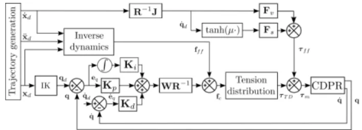
Fig. 10. Dual-space feedforward controller
automatically load and unload goods. The overall dimensions are2 m×12 m×6 m (l×L×h). The real-time control system is based on Beckhoff TwinCAT3 R and runs at a1 kHz sampling frequency. The CPU of the real-time computer is a Intel R
CoreT M2 Duo Processor T9400 @2.53 GHz.
2) COGIRO: This prototype, shown in Fig. 2, is a6-DOF 8-cable suspended CDPR (2 DOR) having a large workspace of overall dimensions15 m × 11 m × 6 m (L × l × h). In the experiments reported in this paper, COGIRO performs pick-and-place tasks, its mobile platform being equipped with a crane fork for a total mass of 93 kg. The control system is based on B&R Automation Studio R running at a1 kHz sam-pling frequency with a CPU Intel CoreR T M2 Duo Processor
L7400 @1.5 GHz.
The paper is accompanied by a video. It first shows the CABLAR prototype moving along predefined trajectories. The COGIRO prototype performing a pick-and-place task is then shown. Both CABLAR and COGIROare controlled by means of the the dual-space feedforward controller of Section VI-B.
B. Dual-space feedforward controller
The dual-space feedforward control scheme shown in Fig. 10 is very similar to the one in [13]. The difference is the use of a joint space instead of an operational spaceP ID controller, the tuning of the former being much simpler in practice.
In Fig. 10, as detailed in [13], the “Inverse dynamics” block compensates for the loaded mobile platform dynamics by means of an operational space feedforward wrench ff f
whereas the actuator dry and viscous frictions Fs and Fv are
compensated for by a joint space feedforward torque τf f.
The termtanh(µ ˙qd) is used to model dry friction in order to avoid discontinuities which may appear with the sign function. Moreover, τm is the actuator input torque vector and τT D is
the torque vector given by the tension distribution algorithm. Let us note that τT D = RtT D, where tT D is one of the
tension distribution solutions of Section IV and R is a diagonal matrix whose nonzero components account for the mechanical transmission ratios and the winch drum radii. The input to the tension distribution block is fc which is the sum of the
feedforward wrench ff f and a wrench generated by the PID
controller [13].
The control scheme of Fig. 10 includes the tension distribu-tion algorithm in the main control loop. If the latter algorithm finds a feasible tension distribution (i.e. (5) is feasible), the corresponding torque τT D is computed. Hence, care must
0 5 10 0 200 400 600 800 1000 1200 Time [s] Tensions [N] Centroid 0 5 10 0 200 400 600 800 1000 1200 Time [s] Tensions [N] Weighted barycenter 0 5 10 0 200 400 600 800 1000 1200 Time [s] Tensions [N] 1−norm 0 5 10 0 200 400 600 800 1000 1200 Time [s] Tensions [N] 2−norm
Fig. 11. Cable tensions measured on the CABLAR prototype, obtained by means of four different tension distributions
the feedforward terms ff f and τf f. Indeed, a bad tuning
leads the P ID controller to overwork making the input fc
to the tension distribution block impossible to balance with feasible cable tensions. Such a situation leads to a failure of the tension distribution algorithm (i.e. Λ = ∅), even if the current trajectory fully lies in the wrench-feasible workspace.
C. CABLAR real-time results
The control scheme of Fig. 10 is applied to the fully constrained CDPR CABLAR with tmin = 150 N and tmax =
1200 N. The mobile platform motion is controlled along a path in the(y, z) plane (i.e. x = 0) with a constant null orientation. They and z coordinates of the waypoints of the path are given in Tab. I. This path is representative of typical intralogistic applications.
TABLE I
CABLAR: WAYPOINTS OF THE DESIRED TRAJECTORY
units: m 0 1 2 3 4 [y z] [0 2] [−2.5, 1] [−2.5, 2.5] [2.5, 2.5] [2.5, 1]
The algorithm of Section III has been implemented and used to compute the four tension distributions presented in Section IV. Fig. 11 shows the measured cable tensions obtained with each method. The corresponding Root Mean Square (RMS) cable tension values are given in Tab. II. As expected, the 1-norm and 2-norm solutions result in lower cable tension values and their RMS tension values are very similar since, along the considered trajectory, λ∗1 and λ
∗ 2 are
always located at the same vertex or at nearby vertices of
the polygonA−1(Λ). The centroid results in the higher RMS
cable tension. As shown in Fig. 11, the weighted barycenter provides an interesting alternative which gives a relatively low RMS tension value compared to the centroid while keeping the cable tensions relatively far from the boundaries of the feasible cable tension setΛ.
TABLE II
ROOTMEANSQUARE CABLE TENSION VALUES OF THE FOUR
CONSIDERED TENSION DISTRIBUTIONS
centroid weighted barycenter 1-norm solution 2-norm solution CABLAR 700.9 N 569.6 N 356.5 N 354.7 N COGIRO 479.7 N 477.2 N ∅ 477.0 N
Tab. III shows the Task Execution Time (TET) of the four considered tension distributions, i.e., for each distribution, the total time needed for the computations of the three steps detailed in Section V-C. For comparison purposes, the TET of an efficient active set method (with warm start) that solves the QP (9) is also given. Tab. III illustrates that the proposed algorithm is efficient since the TETs are slightly larger but comparable to the TET of the active set method. Moreover, contrary to the latter which can only compute the 2-norm solution, the proposed algorithm is versatile since the four tension distributions in Tab. III were computed with the same computer code. To ensure real-time compatibility, the worst-case computation time should be determined. Let us assume that the TET is proportional to the number of FLOPs and let α denote the ratio of time divided by number of FLOPs. The centroid maximum TET given in Tab. III was obtained fornmt= q = 5 which, according to Section V, corresponds
to 1337 + 77nmt + 10q + 24 = 1796 FLOPs whereas
the centroid average TET was in most cases obtained for nmt = q = 4 which corresponds to 1709 FLOPs. The
corresponding values of the ratio α are 0.0127 and 0.0119. The same analysis for the barycenter, 1-norm and 2-norm cases corroborate these values ofα. In the remainder of this section, we thus chooseα = 0.013. Hence, the worst-case TET can be estimated from the maximum number of FLOPs given at the end of Section V-C by multiplying these number of FLOPs by α = 0.013. The results are worst-case TETs of 49.4 µs, 42.3 µs, 41.8 µs, and 44.6 µs for the 2-norm, 1-norm, centroid and weighted barycenter solutions, respectively. This analysis proves that the proposed algorithm easily satisfies the real-time constraint which requires the TET to be smaller than 1 ms (1 kHz sampling frequency). No such worst-case bound is established for the active set algorithm whose TETs are shown in Tab. III. In case of the simple method [19], [35] analyzed at the beginning of Section V-E, an incompressible number of1337 + 3936 FLOPs, which corresponds to 68.5 µs for α = 0.013, is required in order to compute tp, N and
the vertices of A−1(Λ). Adding the computations needed to
calculate the desired tension distributions, the worst-case TET lies in the interval72−80 µs, i.e., four times as much as the TETs shown in Tab. III and twice as much as the worst-case TETs indicated above.
TABLE III
CABLAR: TASKEXECUTIONTIME OF THE TENSION DISTRIBUTIONS
average TET min TET max TET centroid 20.3 µs 18.6 µs 22.8 µs barycenter 21.3 µs 19.1 µs 24.3 µs 1-norm 17.7 µs 16.9 µs 19.1 µs 2-norm 17.7 µs 16.9 µs 18.9 µs active set 14.1 µs 13.4 µs 15.8 µs 10 20 30 40 50 60 0 100 200 300 400 500 600 700 800 900 1000 Time [s] Tensions [N] Centroid
Fig. 12. Motor torques (converted in tensions) of the COGIROprototype obtained with the centroid tension distribution
D. COGIRO real-time results
The COGIRO suspended CDPR prototype is now consid-ered with tmin = 100 N and tmax = 5000 N. The dual-space
feedforward controller of Fig. 10 is used to control the motion of the mobile platform along a trajectory described in Tab. IV, where x = [x y z φ θ ψ]T (XYZ Euler angle convention) defines the pose of the mobile platform.
TABLE IV
COGIRO: WAYPOINTS OF THE MOBILE PLATFORM DESIRED TRAJECTORY
xT [m][o] 0 [0 0 1 0 0 0] 1 [−3.8 1.2 1 0 0 −45] xT [m][o] 2 [−3.8 1.2 0.07 0 0 −45] 3 [−3 2 0.07 0 0 − 45] xT [m][o] 4 [−3 2 1 0 0 45] 5 [4 −1 0.5 0 0 11] xT [m][o] 6 [4 −1 0.07 0 0 11] 7 [4.3 −2 0.07 0 0 11] xT [m][o] 8 [0 0 0.5 0 0 0] 9 [0 0 0 0 0 0]
Nearby the center of the workspace of COGIRO, an edge of the polygon A−1(Λ) turns out to be almost aligned with
the contours of the1-norm objective function (Section IV-B). Consequently, the 1-norm tension distribution is not suitable because the optimal point switches very frequently from one vertex ofA−1(Λ) to another. This results in discontinuities in
the tension distribution evolutions along the trajectory which generate significant platform and cable vibrations.
For the suspended CDPR COGIRO, along the typical tra-jectory given in Tab. IV, the polygonA−1(Λ) is small so that
the three solutions λ∗2, λ∗c and λw are almost identical along
the trajectory. Hence, Fig. 12 only shows the motor torques— in terms of cable tensions—in case of the centroid tension distribution (λ∗c). The corresponding RMS cable tension values
are given in Tab. II. From a general point of view, the centroid may be considered to be the best tension distribution for suspended CDPRs since λ∗c is far from the boundaries of
TABLE V
COGIRO: TASKEXECUTIONTIME OF THE TENSION DISTRIBUTIONS
average TET min TET max TET centroid 24.9 µs 22.1 µs 28.3 µs barycenter 25.8 µs 23.5 µs 29.5 µs 1-norm 21.1 µs 19.7 µs 20.2 µs 2-norm 18.2 µs 17.8 µs 18.3 µs centroid [35] 74.9 µs 75.6 µs 76.8 µs
A−1(Λ), i.e., slack cables should be avoided. However, in the
present case of COGIRO moving along the trajectory given in Tab. IV, selecting the pseudo-inverse solution tp of Eq. (1)
as the desired cable tension distribution is sufficient since the other tension distribution solutions considered in this paper leads to almost the same cable tensions as those in tp.
Tab. V shows the Task Execution Time (TET), i.e., for each of the four considered tension distributions, the total time needed for the computations of the three steps detailed in Section V-C. Let us assume again that the computation time is proportional to the number of FLOPs. The computation of tp and N (step 1 in Section V-C) takes approximately
18 µs. Hence, the constant ratio α of time divided by number of FLOPs is considered to be equal to 0.0135. Accordingly, the worst-case TETs are51.7 µs, 43.9 µs, 43.4 µs, and 46.3 µs for the 2-norm, 1-norm, centroid and weighted barycenter solutions, respectively. These computation time upper bounds satisfy the real-time constraint at 1 kHz. Finally, the last line of Tab. V shows the TET of the centroid tension distribution computation described in [35]. We did our best to implement it as efficiently as possible in the casem = n + 2 = 8, using notably a simple 2D triangulation method [46] (p. 18). These TETs are consistent with the computational cost analysis of this method given at the beginning of Section V-E.
VII. CONCLUSION
This paper introduced a tension distribution algorithm dedi-cated ton-DOF CDPRs redundantly actuated by n + 2 cables. The proposed algorithm first computes the vertices of the convex polygon of feasible cable tension distributions by fol-lowing the polygon edges in a clockwise or counterclockwise order, or it proves that this polygon is empty. Along the way or once all the polygon vertices are determined, it was then pointed out that the optimal 2-norm and 1-norm as well as the centroid and weighted barycenter tension distributions can be directly determined. This results in a versatile algorithm capable of determining various cable tension distributions. Moreover, the proposed algorithm can start at an unfeasible point which eases its use and, importantly, allowed its worst-case computational cost to be assessed. Indeed, the maximum total number of iterations of the algorithm was established and proved to be fairly small. Based on this result, a detailed analysis of the maximum number of floating point operations of the algorithm was provided and compared to some previous methods. This analysis proved the efficiency of the proposed algorithm. This efficiency was also verified by experimenta-tions on the two 6-DOF 8-cable CDPR prototypes CABLAR and COGIRO.