Analyse de l'effet des lacs sur le bilan d'énergie de surface régionale dans le nord du Canada avec l'apport d'images satellites

Département de géomatique appliquée

Faculté des lettres et sciences humaines

Université de Sherbrooke

Analyse de l’effet des lacs sur le bilan d’énergie de surface régionale

dans le nord du Canada avec l’apport d’images satellites

Use of satellite data to esfimate regional surface energy budget and

analysis oflake cover impact over Northern Canada

Vahid Ikani

Mémoire présenté pour l’obtention du grade de Maître ès sciences géographiques (M.Sc.), cheminement Télédétection

May 2009

C

_{Composition du jury}

Analyse de l’effet des lacs sur le bilan d’énergie de surface régionale dans le nord du Canada avec l’apport d’images satellites

Use of satellite data to estimate regional surface energy budget and analysis of lake cover impact over Northem Canada

Vahid Ikani

Ce mémoire a été évalué par un jury composé des personnes suivantes Directeur de recherche Alain Royer

Université de Sherbrooke

Département de Géomatique Appliquée, Faculté des lettres et sciences humaines Lecteur externe : Laxima Sushama

Université du Québec à Montréal (UQAM)

Département des Sciences de la Terre et de l’Atmosphère, Faculté des sciences Lecteur interne Hardy B. Granberg

Université de Sherbrooke

Département de Géomatique Appliquée, Faculté des lettres et sciences humaines

Les lacs occupent environ 30% du territoire dans le nord du Canada. Ils peuvent avoir d’importants impacts sur le climat qui ont un effet par la suite sur les propriétés thermiques des lacs. L’étude d’un lac doit généralement débuter avec un bilan calorifique de la surface. La différentiation précise que l’énergie disponible en flux de chaleur sensible ou latent est un élément crucial pour la compréhension des interactions entre les processus climatiques à une échelle régionale.

Dans cette étude, le flux de chaleur sensible et le ratio de Bowen sont obtenus à partir des données de la télédétection. La méthodologie se base sur l’utilisation de données micro-ondes (SMM/I) afin de calculer la température de la surface du sol avec la méthode de Fily et al. (2003) et Mialon et al. (2007). La caractérisation de la surface du sol est effectuée à partir de données satellitaires optiques (capteurs SPOT & VGT). Les paramètres météorologiques utilisés pour estimer les flux proviennent de la base de données du North American Regional Reanalysis (NARR).

Les résultats présentent un portrait quotidien, mensuel et saisonnier de l’énergie sensible à l’interface sol-air par rapport à la fraction de la surface de plan d’eau (FWS). Nous comparons ensuite nos résultats avec les flux du modèle NARR et quelques mesures in situ.

Quatre sites couvrants différents types de surfaces à travers le Canada ont été étudiés pendant les étés 1998 et 2000 (de juin à septembre) : le nord du Québec (toundra), les Territoires du Nord-Ouest (le Grand lac des Esclaves [ou, en anglais, Great Slave Lake

-GSLJ et le bassin de la rivière Mackenzie), le Manitoba (zone humide) et le Labrador (taïga).

Les résultats montrent que les flux d’énergie sensible satellitaires sont semblables aux flux estimés par le NARR lorsque la FWS est petit (sans lac) ou pour des zones avec de larges surfaces d’eau (Mackenzie Great Slave Lake), mais diffèrent lorsque la FWS augmente à l’intérieur d’un pixel. Ceci signifie que les modèles climatiques régionaux devraient considérer la proposition du territoire occupée par des étendues d’eau. Nous déduisons que les effets de la taille des lacs sont reliés aux conditions environnementales du milieu. Les résultats de la comparaison avec des mesures in situ pour le GSL et la zone humide sont encourageants.

Le ratio de Bowcn sur le site du bassin de la rivière Mackenzie montre qu’il y a une augmentation de la chaleur sensible durant la deuxième moitié de l’été en comparaison à la première moitié. Il y a ainsi un plus grand stress hydrique pendant la deuxième moitié de l’été. Cependant, il n’y a pas de patrons clairs en comparaison avec le site GSL. La comparaison entre les différents sites indique une variation énergétique annuelle minimale pour la zone humide.

Mots-clés : Modèle climatique régional, Micro-ondes passives (SSMJI), Flux de chaleur sensible, Ratio de Bowen, FWS, Température de surface normalisée, Résistance de bulk.

Abstract

Lakes occupy roughly 30% of Canada’s northem landscape. They can have important impacts on the climate, and climate modification wilI affect lake thermal properties. Study of a lake most generally begins with heat budget at its surface. Accurate partitioning of die available energy at the surface into sensible and latent heat flux is crucial to the understanding of interactions between climate processes on a regional scale. In this smdy, sensible heat flux and the Bowen ratio for the summer pedod are retrieved using reanalysis and remote sensing data. fle methodology is based on the use of microwave data for retrieving land surface temperature (SSMII) with the method of Fily et al. (2003) and Mialon et al. (2007). The land cover characterization is derived from remotely sensed optical data (SPOT VGT sensor). Some meteorological parameters used for retrieving flux are derived from the North American Regional Reanalysis (NARR) database.

The resuits from this study present a picture of the daily, monthly and seasonally sensible energy over summer period at the land-air interface versus the Fraction of Water Surface (FWS). We compare our resuits with the NARR model’s flux in addition to few in situ measurements.

Four sites covering different land cover types across Canada were investigated during the 1998 and 2000 summers (June to September): Northem Quebec (tundra), Northwest Territodes (Great Slave Lake, or GSL, and Mackenzie River Basin), Manitoba (wetlands) and Labrador (taiga).

The results show that the satellite-derived sensible flux is close to the NARR flux estimate when the fraction of water surface is small (no lakes) and over large open water areas (Mackenzie Great Slave Lake), but differs when the FWS increases within the pixel. This means that regional climate models should take into account lake cover fraction. We infer that effects of the lake-size are closely related to sunounding environmental conditions. The results of the comparison with in situ measurements for Great Slave Lake (1998) and the Wetland site are encouraging.

For the Mackenzie River Basin site, the results of the Bowen ratio show that there is an increase of sensible heat partition during the second half of the summer in comparison with the first hait’, meaning that there is more water stress over the second haif of the summer than the first. But for the Wetland site, there is no clear pattem, and in comparison with GSL, temporal variation is less significant. Comparisons between different sites indicate minimum year to year energy variation for the Wetland area.

Keywords: Regional climate model, Passive microwave SSM/I, Sensible heat flux, Bowen ratio, Fraction of Water Surface, Normalized Surface Temperature, Bulk resistance.

Table of contents y

List of figures vii

List of tables ix List of Appendix ix Glossaiy x 1. Introduction 1 1.1 Problem 1 1.2. Objectives 7 1.3. Hypothesis 7 1.4. Plan 8

2. The energy budget constraint 8

3. Site description 11

4. Data description 12

5. Methodology 14

5.1 Data processing 14

5.1.1 Temperature derived from satellite measurements 16

5.1.2 Determination of fractional water surface 16

5.1.3 Satellite-derived temperature daily normalization 17

5.1.4 Image processing 18

5.1.5 Extraction the NARR data 19

5.2 Retrieval of sensible heat flux from satellite data 20

5.2.1 Retrieved sensible heat flux 20

5.2.2 Estimation of latent heat and Bowen ratio 24

5.3 Temperature condition 25

6. Results 25

6.1 Comparison between retrieved and modelled sensible heat flux 25

6.2 Importance oflake size 33

6.3 Seasonal (rnonthly) sensible heat fluxes variation 35

6.4 Site to site Comparison 41

6.5 Comparison between 1998 and 2000 47

6.6 Bowen ratio estimation— “GSL” and “wetland” sites 49

6.7 Compadsons with in situ measurements 50

7. Conclusions and verification ofhypothesis 57

8. References 58

1. Lake —wide average sensible and latent heat flux in 1999

(Great Slave Lake and Great Bear Lake) 4

2. Direction of sensible heat fluxes 9

3. Schematic figure ofthe heat budget ofa thin interfacial layer near the surface

(Source: Sun et al., 1995) 10

4. Location ofthe study sites 11

5. A quick view of the data and acquired sources 14

6. Algorithm used for study 15

7. Normalization process: applying ERA-40 diumal cycle (dashed line) to satellite-derived temperaffire (x) derived from SSMJ I sensor leads to

nomialized (hourly) series (continuous) 18

8. Land cover classification ofNorth American year 2000(Latifovic et al., 2002) (a) EASI-Grid projection and (b) visualization the same figure

in geographical coordinates 19

9. Schernatic description ofmodels for heat transfer (source: Lia 2004) 21 10. The daily variation of sensible heat as a ifinction ofFWS for the GSL

site - August 1998 26

11. The daily variation of sensible heat as a flrnction ofFWS for the GSL

site - August 2000 27

12. The daily variation of sensible heat as a flinction ofFWS for the GSL

site- July 1998 28

13. The daily variation of sensible heat as a fiinction ofFWS for the GSL

site - July 2000 29

14. Average sensible heat flux versus FWS%, GSL 31

15. Average sensible heat flux versus FWS%, Wetland 32 16. Daily values of sensible heat flux for GSL site for SL, ML and LL

Classes separately, July and August 1998 34

17. Average surface-air temperature gradient versus FWS% for four

months (July, August and September) of 1998 and 2000 for the GSL 37 1 8. Average sensible heat fluxes (retrieved) versus FWS% for four months

(June, July, August and September) of 1998 and 2000 for the GSL 37 19. Average surface-air temperature gradient versus FWS% for four months 38

(July, August and September) of 1998 and 2000 for the Tundra 20. Average sensible heat fluxes (retrieved) versus FWS% for four rnonths

(JuIy, August and September) of 1998 and 2000 for the Tundra 38 21. Average surface-air temperature gradient versus FWS% for four

rnonths (June, July, August and September) of 1998 and 2000 for the

Wetland 39

22. Average sensible heat fluxes (retrieved) versus FWS% for four months (June, July, August and September) of 1998 and 2000 for the

Wetland 39

23. Average surface-air temperature gradient versus FWS% for four months (June, July, August and September) of 1998 and 2000 for the

Taiga 40

24. Average sensible heat fluxes (retrieved) versus FWS% for four months

(June, July, August and September) of 1998 and 2000 for the Taiga 40 25. Comparison between the 4 sites - modelled and retrieved values over

the summers of 1998 42

26. Comparison between the 4 sites - modelled and retrieved values over

the summers of 2000 43

27. Cornparison between 4 sites, over 1998 and 2000, SF cJass 47 28. Comparison between 4 sites, over 1998 and 2000, MF class 48 29. Comparison between 4 sites, over 1998 and 2000, LF class 48 30. Bowen ratio as a fiinction ofFWS for the GSL—years 1998 and

2000 51

31. Bowen ratio as a fiinction of FWS for the wetland—years 1998 and

2000 52

32. Spatial distribution of the H/R ratio for the “GSL”, rnodelled and

Retrieved 54

List of tables

1. List of studies related to surface flux measurement derived from

Jiang et al., 2004 6

2. The geographical coordinates ofthe study sites 12 3. Name of sites and close meteorological stations 25

4. Ratios (yir) for GSL site 45

5. Ratios (vit) for Wetland site 45

6. Ratios (vit) for Tundra site 46

7. Ratios (y/x) for Taiga site 46

8. Bowen ratio values for the GSL site 50

9. Bowen ratio values for the wetland site 50

10. Comparison ofH/R110 ratio within situ (Rouse et al., 2001)- GSL 53 11. Comparison ofH/R ratio with in situ (Rouse et aL, 2001)- wetland 55

List of appendix

Appendix 1- Classification of land covers 66

Appendix 2- Values of aerodynamic roughness 67

Appendix 3- Temperature condition for the study sites 68

Appendix 4- The retrieved values for GSL site 69

Glossary

AVHRR Advanced Very High Resolution Radiometer

CRCM Canadian Regional Climate Model

C Air specific heat at constant pressure

(

₎

KgK

d Zero plane dispiacement (m)

DMSP Defence Meteorological Satellite Program

w

E Latent heat

_(—-)

In

-EASE Grid Equal Area Scalable Equal Area

Emissivity at horizontal polarization

Emissivity at polarization p

Emissivity at vertical polarization

ew Ernissivity of water

FWS Fraction of water surface

G Ground heat flux

(tÇ)

ni

G Gravitational acceleration

GCM General Circulation Model

GSL Great Slave Lake

Canopy Height (ni) H Sensible beat flux

_(—-)

‘n

K Kofeman Coefficient (Dimensionless)

kW’ Excess resistance parameter (Dimensionless)

L Obukhov stability length (rn)

w

L4. Incoming long wave radiation

_(—-)

ni

[4

Outgoing long wave radiation

_(—-)

‘n

LF Large Fraction of water surface MAE Mean Absolute Error

MF Medium Fraction ofwater surface

MRB Mackenzie River Basin

NF No Fraction of water surface

NARR North American Regional Reanalysis

NCEP National Center for Environment Prediction

NSIDC National Snow and Ice Data Center

POM Princeton Ocean Model

w

Net radiation flux

_(—-)

‘n

ra Aerodynarnic resistance

(—e-—)

‘n

w

S Outgoing short wave radiation

_(—-)

‘n

54. Incoming shortwave radiation

_(—-)

in

SF Srnall Fraction ofwater surface SSMII Special Sensor Microwave Image

Ta Airtemperamre (KO)

Tb Downward atmospheric contribution

Tau Upward atmospheric contribution

TBH Apparent brightness temperamre at horizontal polarization (satellite level)

TBV Apparent brightness temperature at vertical polarization (satellite level)

TB Apparent bdghtness temperature at satellite level

Surface temperature

(KO)

PI

U Wind velocily in X direction

_(—)

s

ni

V Wind velocity in Y direction

_(—)

s

W Wind speed

_(-)

-—

s

Z Reference height Aerodynamic roughness Iength (rn)

Stability correction fiinction for heat transfer (Dimensionless)

Stability correction fiinction for momentum transfer (Dimensionless)

fi

Bowen ratio (HI (R0 -W) (Dimensionless)

p Air density

₍

ni

Remerciements

Je tiens à remercier en premier lieu le Professeur Alain Royer pour son soutien scientifique, ses avis, ses encouragements, sa patience et sa bonne humeur.

Je tiens aussi â exprimer ma reconnaissance au Conseil de Recherches en Sciences Naturelles et en Génie du Canada qui a permis de financé cette recherche.

Un grand merci à l’équipe DAT (Donnée Accês Intégration) pour les donnes de NARR, la Cartothèque de l’université de Sherbrooke et Stéphane Poirier de l’équipe de Royer et GEC3.

An understanding of the energy budget of lakes and wetlands and their interaction with the atmosphere is crucial for assessing the impacts of resource development and climate change (Long et ah, 2007). In recent years, various stadies have been conducted to estimate surface energy fluxes using remote sensing techniques. Remotely sensed data are the only tools that have the potential to provide spatially distributed information relating to land surface parameters and state variables on a regular basis, on a range of spatial scales. This information is potentially very usefiil in hydrology and meteorology for quantifying the spatially distributed parameters and variables that control the interaction of land surface and atrnospheric processes (Humes et aI., 1997).

In this study we estimate sensible heat flux and its variations as a ffinction ofthe Fraction ofWater Surface (FWS). For the purpose ofthis smdy, based on method Puy et al (2003), Mialon (2005) and SSMft data, an algorithm for estimating sensible heat flux svas developed. The SSMII data are applicable any time of day, in ail weather conditions, and provide a resolution of25 km. In the following section, the problem wiiIl be discussed. The objectives and hypotheses are then explained. Finally, we present the plan of the thesis.

1.1 Problem

Canada has nearly two million fresh water lakes ranging in size from less than 1 km2 up to some of the largest lakes in the world. The lakes occupy roughly 30% of Canada’s northem landscape. Because oftheir abundance, lakes are important factors pertaining to the regional climate. Air and water exchanges of heat and moisture have climatological implications not only on water bodies but also on the climate ofthe overlying air and the areas adjacent to water masses (Long et aI., 2007).

Swayne et al. (2004) indicated that the inland water (lakes, wetlands) can have important impacts on the climate on various spatial scales; also, climate variations wilI affect lake

2

thermal properties. Furthermore, Nagarajan et aI. (2004) conclude that small lakes have a substantial effect on the atmospheric heat and water budgets.

On the other hand, understanding of the physical characteristics and processes of Canada’s northem lakes is poor, and the impact of numerous small lakes on regional weather and climate is even less well known (Spence and Rouse, 2002).

Much research on the physical climatology of lakes has focused on the variation of heat and moisture exchanges at the air-water interface. The study of a lake begins with the heat budget at its surface, and the fluxes of heat Ihrough the lake-atmosphere interface is the major source and sink for the heat involved in the thermal processes (Dutton and Biyson, 1962). Furthermore, one of the most recent studies by Mommi and Ito (2008) indicates that the study of the heat budgets of lakes is an essential component of efficient lake-water management as it gives direct information on evaporation, thus on an important component ofthe lakes’ water budget.

Inclusion of a ffihly interactive lake model in the regional climate model is an important objective of the Canadian Regional Climate Modeling and diagnostics (CRCMD) network. The North American Regional Reanalysis (NARR) only considers large lakes and not small lakes in the process. Lake surfaces have very different interactions with the atmosphere, as compared to land surfaces, particularly moisture evaporation, wind forcing and energy exchanges. These air-water interactions, however, are complex and continue to be a critical issue considering the millions of lakes in Canada that are neglected in the curent clirnatic models (Swayne et al., 2005).

In order to examine the interaction between northem lakes and surrounding regional atmosphere, Long et al. (2007) used the atmosphere-lake coupled model. The Princeton Ocean Model (POM) was coupled to the Canadian Regional Climate Model (CRCM) for Grcat Bear Lake and Great Slave Lake. The simulated sensible and latent heat fluxes in July and August 1999 (without and with lake) are shown in Figure 1.

o

r E D t, L V L V. z V u, (a) C’ E X D w t, V n V n la = V (M (b) X D w q t, V n q C V (c) X D w ØV V n C V (d)

Figure 1. Lake-wide avcraged sensible heat flux in 1999: (a) Great Bear Lake, (b)Great Slave Lake and averaged latent heat flux, (e) Great Bear Lake, (d) Great Slave Lake; simulations without (dashed) and with (solid) lakes (Source: Long et al., 2007)

4

Uncoupled simulations (without lake) resuit in overestimation ofthe surface sensible and latent heat fluxes in summer (July-August) and underestimation of these surface heat fluxes in October. fle associated summer overestimation in the surface sensible heat fluxes is more than 50W/m2 and the October underestimation, by more than 50W/rn2 (Figs. la and lb). In addition, uncoupled simulations resuit in a summer overestimation in latent heat transport from the lake surface (as estimated from surface evaporation), by about 1 OOW/m2, and an October underestimation by about 50W/rn2 (Figs. 1 c and 1 d). Therefore, the impacts of northem lakes on regional surface heat exchange between the lakes and the atmosphere are significant.

To better understand the exchange of heat and moisture between the surface and the lower atmosphere, it is important to quanti the components of the surface energy balance in a distributed fashion on the landscape scale (Segal and Arritt, 1992).

In this study sensible heat flux is quantified. Sensible heat can be used to verify climate and weather models and is necessary for regional studies of lakes and also desertification (Bolle, 1997). Accurate representation of sensible heat is beneficial to compute the heat flux in Numerical Weather Prediction (NWP), General Circulation Models (GCM) and to develop surface flux data sets (Cao et al., 2006).

Furthcnnore, accurate partitioning of available energy into sensible and latent heat flux (Bowen ratio) is crucial to the understanding of surface-atmosphere interaction. Bowen ratio is critical in determining the hydrological cycle, boundary layer development, weather, and climate. For example, Bowen ratio can be interprctcd as an indicator of water stress.

The search for methods for estimating sensible and latent heat fluxes using low-cost, transportable and robust instrumentation constitutes a subject of interest (Castelivi et aL, 2006). The measurement of turbulent fluxes requires sophisticated instruments. These measurements have been mainly confined to intensive fleld expedments. The direct method is expensive and complicated. When performed over a water surface, for example over a lake, these measurements are usually more difficuit to obtain with great accuracy, and few direct measurements ofthese fluxes are available (Rouse and Spence, 2003).

Table 1 provides a Iist of studies related to the issue of surface flux measurement. We must emphasize that this is a representative set ofprevious studies, flot an exhaustive Iist ofearlier work (Jiang et al., 2004).

Because there are not enough data and meteorological stations, remotely sensed data are tools that have the potential to provide spatially distributed infonnation. Before the advent of satellite technology, the surface fluxes, especially sensible heat fluxes and latent heat fluxes, had to be calculated exclusively relying on in situ measurements. Kampf and Taylor (2006) indicate that remote sensing is usefiil for identil’y’ing spatial pattems not apparent from point measurements on the ground, and it provides important insight into land surface energy budget analyses.

Therefore, understanding the energy budget of lakes and wetlands and their interaction with the atmosphere is crucial for assessing the impacts of resource development and climale changes. fle current regional climate model without accounting for water

components, overestimates the heat transfers when forecasts are performed in lake- or wetland-covered areas. Although several surface-based methods accurately measure surface energy fluxes at point locations, the spatial vadability of the fluxes limits their application to larger spatial areas. With satellite technologies, we now have a complementary way to remotely derive surface fluxes with uniform spatial and temporal samp ling.

6

Table 1. List of studies related to surface flux measurement derived from Jiang et al., 2004

Reference (Derived from Jiang et al.,2004) Technique, case study or experience Blad and Rosenberg (1974)

Soer (1980)

Kustas et aI. (1989)

Dugas et al. (1991), Fritschen et al. (1992), Kustas and Norman (1997) Stewart et al. (1994)

Kustas et al. (1994)

Pelgrum and Basliaanssen (1996) Eichinger et aI. (1996)

Moran et al. (1996)

QuaIls and Bmtsacrt (1996)

Bastiaanssen et al. (1998) Gao et al. (1998)

Kustas et al. (1998)

Ibanez et al. (1998; 1999) Kustas et al. (1999) Kustas and Jackson (1999)

Mecikalski et al. (1999)

Castelli et al. (1999) Nishida et al. (2003) Norman et al. (2003)

Aerodynamic formulation for H(adjusting kBj MetFlux observation

Different methods for area-avemged KE with remote sensing data Priestley-Taylor method

Trapezoidal method

Evaluation of ground-based and remotely sensed data to estimated spatially distributed sensible heat fluxes (FIFE measurements) “Triangle” method for sou moisture and surface fluxes from remote fluxes from remote sensing

SEBAL algodthm with remote sensing data at HEIFE

Comparison ofestimated Cloud and Radiation Testbed (CART) average and EBHR-derived average fluxes

Comparison between dual-source model and observations of instantaneous surface fluxes

Radiative Bowen ratio model

Atmosphedc boundary layer data and remote sensing data, N95 model Impact on area-averaged heat fluxes using remote sensing data at different resolutions (Washita’92)

ALEXI model and Geostationary Operational Environmental Satellite 8 (GOES-8) data

Variational data assimilation approach (adjoint technique) (FIFE) Simple two-source model of ET, combined with T—VI diagram Twn-source model DisALEXI and combination of Iow- and high resolution remote sensing data

Bowen ratio melhod

Residual method for regional evapotranspiration Residual method with thermal infrared data Bowen ratio and eddy covariance systems

Carlson et al. (1995), Gillies et al. —l997)

1.2. Objectives

The objectives ofthis research are to:

• Derive sensible heat fluxes on a daily, monthly and seasonal basis as fractional values of water surfaces by combining satellite and model data at a resolution of

25 x 25 km2.

• Analyse the impacts of northem lakes on the regional energy cycle; develop and improve the cotuprehensive picmre of the seasonal thermal and energy regime (sensible heat fluxes) and its variability over lakes and wetlands.

• Analyse the impact of a very warm summer (1998 — the year when BI Nino

occuned) on the energy budget over northem areas.

• _{As a specific objective, we will examine the error in the energy exchange}

calculation between the atmosphere and land that may occur in the North American Regional Reanalysis (NARR) data due to the presence ofsmall lakes.

1.3. Hypotheses

• To verii’y if the Fraction of Water Surface (FWS) modifies the surface sensible heat flux. The tuore the FWS increases, the more the sensible heat flux decreases, but this impact is seasonally variable. We hypothesize that this effect is more important during late summer in comparison to the early summer period.

• In the second half of the summer, the increasing sensible heat is greater than the increasing latent heat. Therefore, the Bowen ratio of the second half is greater than the first halL

8

1.4 Plan

The organization of the thesis is as follows: the next section describes the concept and theory of energy fluxes and turbulent energy, then the subsequent section presents the site and data descriptions of the study. The section thereafter presents the rnethodology. The penultimate section describes the resuits and hypotheses verification, and the final section contains the summary and conclusion.

2. The energy budget constraint

The turbulent fluxes of water vapour and sensible heat near the Earth-atmosphere interface are linked not only by similarity relationships in the turbulent air, but also by the energy budget. Indeed, both evaporation, as a latent heat flux, and the related sensible heat flux, require the supply of some other forms of energy. Therefore, their magnitudes are constrained by this available energy. Energy equation can be treated quantitatively by considering the energy budget for the layer of surface Énatenal. Depending on the nature ofthe surface, this layer may consist ofwater, or ofsome other substrate like soil, plant canopy or snow (Bnitsaert, 2005).

There are essentially four types ofenergy fluxes at the surface:

The net radiation (W/m2); sensible heat: H (W/m2); latent heat: L (W/m2); and the flux

mb

or out of sub-medium soil or water: G (W/m2). The energy budget equation can be written as (Arya, 2000):

R01=H+L+G (1)

The sensible heat flux (H) at and above the surface arises as a result ofthe difference in the temperatures of the surface and the air above. In the case of sensible heat transfers, a temperature gradient must exist between the surface and the subsurface for a heat transfer to occur (Arya, 2000).

Sensible heat fluxes in lake surfaces play an important rote in the energy balance between lakes and the atmosphere. The sensible heat flux is the direct physical contact of the atmosphere and lake, and enables energy to be exchanged between them by conduction (Bigg, 1996).

Through sensible heat fluxes, the lake absorbs (releases) the heat energy from (to) the atmosphere, compensating for the sharp temperature change in the atmosphere and adjusting the local clirnate and beyond (Pan et ai., 2003).

We used the sign convention that ail the radiative fluxes directed towards the surface are positive, while other (non radiative) energy fluxes directed away from the surface are positive. Figure 2 shows the sensible heat flux away from (positive) and toward (negative) the surface.

H+4

_H*

Figure 2. Direction of sensible heat fluxes

The latent heat flux (L) is a resuit of evaporation, evapotranspiration or condensation, and the rate of evaporation or condensation at the surface. Evaporation occurs from water surfaces as well as from moist soil and vegetation surfaces whenever the air above is drier, i.e., it has iower specific humidity than the air in the immediate vicinity ofthe surface and its transpirating element (Arya, 2000).

The ground heat flux (G), to or from the sub-medium and heat, is transferred via conduction (Aiya, 2000). This flux is a small, but not insignificant, component of the surface energy budget. This flux is also relatcd ta the surface temperature (StulI, 1998).

Q

10

The net radiation (R) absorbed by the surface is the sum of the net shortwave (solar) and long wave (thermal) radiations:

R11,= (S S1) + (L -L1) (2)

81 and S are the respective incoming and outgoing (or reflected) shortwave radiations,

and L1 and L1 are the respective incoming and outgoing long wave radiations (Aiya, 2000). Figure 3 shows a schematic figure of the heat budget near the surface. The energy incoming into a layer adjacent to the ground, the so-called available energy

(R0 — G), must be divided behveen sensible heat (H) and latent heat (L) energy

(Manilo, 1989).

[idownward

I

short- and long-I

wave radiatioj turuience)

___7

obs. surface, z=O

L

J,

air

I

conduction

m

ground

_HQ

absorbed radiation (Anet)

E

LL.0

Figure 3. Schematic figure of the heat budget or a thin interfacial layer near the surface (Source: Sun et al., 1995)

3. Site description

Four different vegetation types were selected for this study, ranging from mature forest to tundra. Figure 4 shows the locations of the sites. The four sites used in ibis study are as follows:

The first site is some parts of Great Slave Lake (GSL) and Mackenzie River Basin (MRB) in the Northwest Teritories. Lackman and Gyakum (1996) reported that evaporation over the MRB exceeds adjective transport of moisture during the summer season, suggesting that the MRB is in itself a significant source of moisture and a suitable place for orographie or lee-cyclogenesis and front genetic processes which influence the east of Canada. The dominant land cover type at this site is boreal forest. This thesis refers to the site as

t..-. s... C L bI Edmonton * Tomme Fv.dtilcion o t o

12

The second site is Iocated in northem Manitoba, south of Hudson Bay. This region is characterized by dominance of wetland areas. Understanding the energy exchange of wetlands is important because it affects radiative and temperature regimes, water transport, plant growth, and productivity (Burba et al., 1999). This thesis refers to this site as “Wetland.”

The third site is located in north-westem Labrador. The area is very important in the field of hydrology, and this region is characterized as Taiga (open forest), Tundra and a number of small bodies ofwater. The thesis refers to this site as “Taiga.”

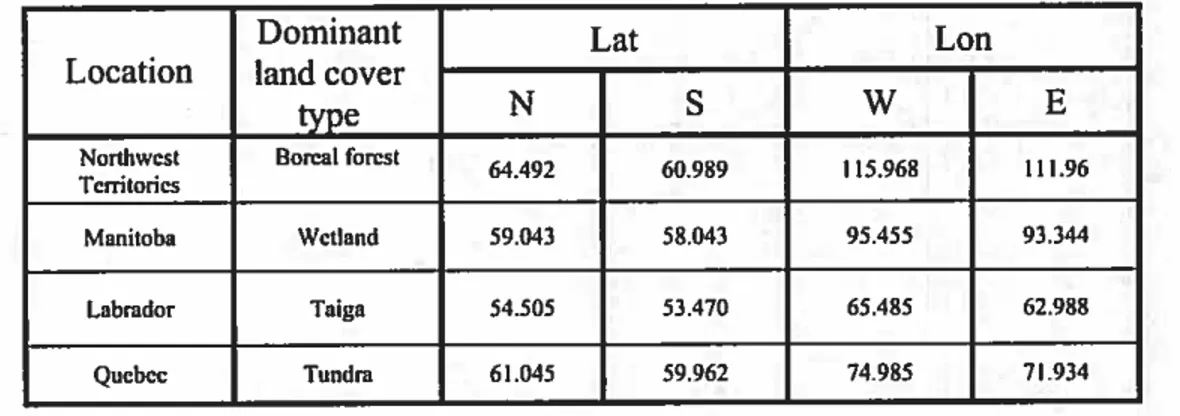
The fourth site, located in the northem Quebec, k covered with tundra. The tundra area has a unique water cycle due to the presence of frozen ground (Kodama et al., 2007). The distribution of low vegetation, such as lichens, moss, and sedge, also plays an important role in surface energy over the tundra watershed (Sato, 2004). This research refers to this site as “Tundra.” The geographical coordinates of the sites are given in Table 2.

Table 2. The geographical coordinates of the study sites

Dominant _{Lat Lon}

Location land cover

type N S W E

Northwcst Borcal fowst _64.492

60.989 115.968 111.96 Tenilofles Maniloba \Vciland 59043 58043 95455 93.344 Labrador Taga 54.505 53.470 65485 62.988 Quebec Tundra 61.045 59.962 74.985 71.934 4. Data description

The estimation of surface sensible heat fluxes can be accomplished through several methods. Most of these methods usually require key input parameters such as air

temperature, wind speed and surface temperature (StuIl, 1988). Furtherniore, estimation energy flux requires the combination of data from several sources. In this study, there are three essential sources of data.

The flrst source is the remote sensing. We used the data provided by the Special Sensor Microwave Imager (SSMJI). The SSMR is onboard the Defence Meteorological Satellite Prograin (DMSP), a satellite series that visits the same part of the Earth’s surface twice a day. Passive microwave measurements are independent of solar illumination, and infornrntion from the surface can be acquired even through clouds as opposed to optical sensors (FiIy et aI., 2003).

The pixel spatial resolution depends on the frequency measured. However, in the re sampled Northem Hernisphere Equal Area Scalable (EASE-Grid) format, the data are readily available at a resolution of 25 km. These data are distributed by the National Snow and tee Data Center (NSIDC), located in Boulder, Colorado (USA). Our research is restricted to the 19.35 and 37 GHz frequencies, as they are less affected by atmospheric effects. Oniy the 37 GHz are used from this point on because the penetration depth is smaller than it is for the 19.35 GHz channel, making it sensitive to soil moisture, and because the spatial resolution at this frequency is doser to the EASE Grid resolution: 27 km x 18 km at 37 GHz as opposed to 69 km x 43 km at 19.35 GHz. In addition, we used the land-cover database of North America for the year 2000. It ïs generated jointly by the Canada Centre for Remote Sensing (Naffiral Resources Canada) and the US Geological Survey. It was compiled using SPOT VEGETATION data at the spatial resolution of 1 km land-cover type.

The second source of data is the North American Regional Reanalysis (NARR). The North American Regional Reanalysis is a reprocessing of the histodcal meteorological observations using National Centers for Environmental Protection NCEP’s regional climate model. The NARR project was completed in 2004. NARR products are in GRIB format on a Lambert conformai conic grid (32 km) at 29 pressure levels.

14

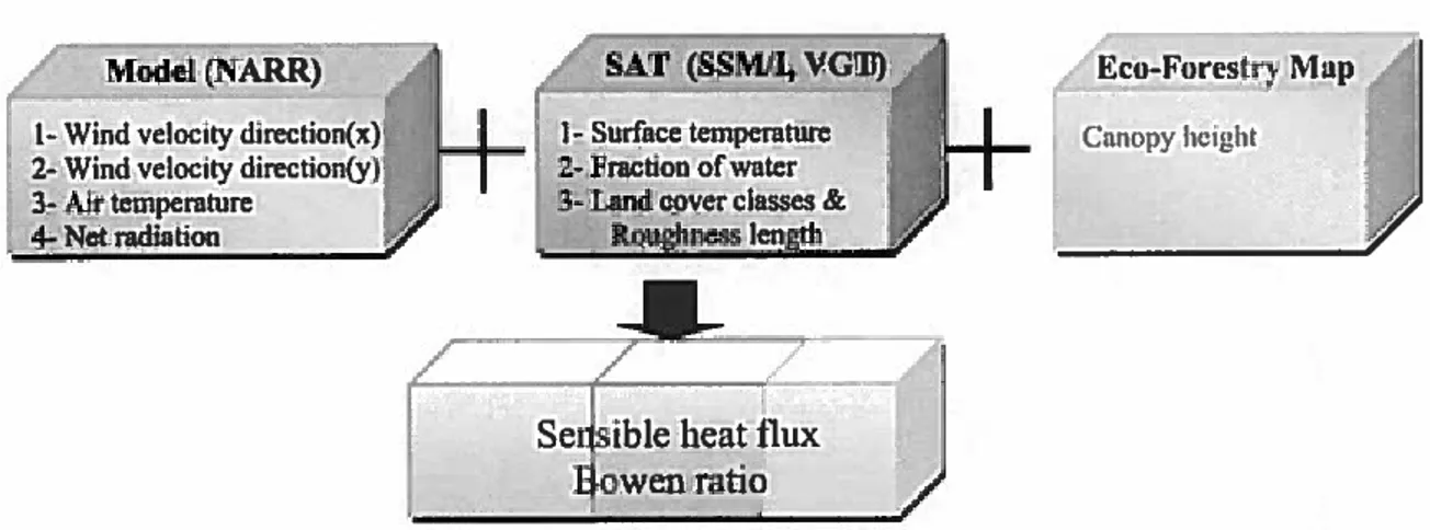
They were produced using a 45-layer topography model. The NARR is a long-term, dynamically consistent high-resolution, high-frequency atrnosphedc and land surface hydrology dataset for North American domain (Mesinger et al., 2006). The output analyses are 3-hourly with 9 additional variables in the 3-hour forecasts to reflect accumulations or averages.Finally, we used an Eco-forestry map in order to find the canopy height. Figure 5 shows bdefly data and acquircd sources.

4

Model(NARR) 14SAT(SSM/IVGTJ Eco-Forestr

1- Wind velocity direction(x)r4______ j i-Surface temperature L...L... (unopvIici”hl

2- Wind velociLy direction(y)i1I “ 2- Fraction ofwaier

3-Air tempenture 3- Land cover classes &

4- Net radiation Rai ness Iength

Sedsible heat flux Bowen ratio

Figure 5. A quick view of the data and acquired sources

5. Methodology

Based on satellite remote sensing data (SSMJI and SPOT VOT sensors), the NARR model and the atmospheric boundaiy layer, the methodologies to determine sensible heat fluxes and the Bowen ratio are deduced. Figure 6 shows the algorithm used for this study.

The methodology is divided into hvo essential parts: the first part is data processing and the second partis retrieval processing.

5.1 Data processing

In this part we extracted surface tempemture, FWS, atmosphcric temperawre, wind speed, net radiation, and land surface characteristies:

r1

summer1998-2000

satellite SSMR SPOT VEGETATION

16

5.1.1 Temperature derived from satellite measurements

At a given polarizationp, for any ftequency, the apparent brightness temperature TB at satellite level can be written (Fily et al., 2003):

TB =epxtxï +Q—ep)xixl +I,,

(3)

Where

ep

is emissivity at polarization p, t is atmospheric transmission, Tab is downward atmospheric contribution, Tau is upward atmospheric contribution, T5 is land surface temperature.

Bdghtness temperature consists of gridded data in an EASE-Grid projection. They are provided at a 25 km resolution at a given location in our station area: up to two measurements per day are available.

5.1.2 Determination of Fraction of Water Surface (FWS)

Assuming a linear relationship between emissivity at vertical polarization (ev) and emissivity at horizontal polarization (eH )as suggested by Fily et al. (2003) such as e-=ae +b (a=OE5022 and b0.4838 at 37 0Hz) we can eliminate the unknown emissivity from the relation (3), the surface temperature is (Fily et al., 2003):

T = (TBV —

o x TBH

— (i — b — a)x t x T x T,,

x

(i — a))

(4)

(txb)

Where TBV and TBH are the apparent brightness temperature at polarization vertical and horizontal respectively. We then obtain two sets of temperatures (T5 - 19 and T5

-27), one for each frequency; from Equation 4, the ernissivity can be cornputed as:

(TB —txT

_Tad)

ep=

(5)

And finally, the fraction ofwater surface (FWS) in the obsewed pixel (Fily et aI., 2003): (6)

(ew- ediy)

where ediy is the emissivity ofa dry surface and

ew

is the emissivity ofwater. The FWS includes surface bodies of water, saturated wetland swamps, marshes, or fens. Therefore, based on FiIy et al. (2003), the FWS values are aggregated at a 25 x 25 km pixel resolution on the EASE-Grid geographical projection.

5.1.3 Satellite-derived temperature dally normalizafion

Remote sensing images record a snapshot in time, whereas land surface energy fluxes change continuously. In this study, since a maximum of only two temperamres can be derived daily from satellite overpasses, it is difficult, it is difficult to compare satellite derived temperatures with other climatic sources based on mean daily. In order to obtain the daily mean surface temperature, the method proposed by Mialon (2007) was used to extract the Nomialized Surface Temperature (NST).

A normalization approach based on the 40-year ECMWF reanalysis (ERA-40; 2.5° resolution) temperature diumal cycle fitted for each pixel is applied to overcome the time acquisition variation of measurements as well as to interpolate missing data. An adaptive mask for discriminating between ice-free pixels and snow-free pixels is also applied. The resulting database is thus a new consistent hourly series of near-surface air temperatures during the summer (without snow). For consistent time sedes, it is necessary to accurately interpolate the gaps between measurements by taking into account the diumal cycle(Mialon et al 2007).

ERA-40 air temperatures are available eveiy 6 h at a spatial resolution of 2.5°. An hourly diumal cycle is obtained from ERA-40 data interpolated with a spline cubic ffincfion (Mialon et al., 2005).

18

This interpolation technique has the advantage of producing smooth sedes at measurement points. The principles of this approach are presented in Figure 7. One or two AT (i.e. Tsat minus ERA-40 temperature interpolated at a given hour) are available every day. A linear interpolation is then used b obtain hourly AT series. Adding hourly AT series to hourly ERA-40 temperature sedes results in an hourly temperature series (hereinafter referred to as normalized temperature norm) fitted with satellite derived temperatures from Equation 4 (Mialon et al., 2005).

Diumal variation model fromERA4OaIr

A _{f temperature} A

st4,r

J

L

lime _lime

a)

b)

Figure 7. Normalization process: applying ERA4O diurnal cycle (dasheil Ihie) to satellite-derived temperature (x) derived from SSM/ I sensor Ieads to normalized

(hourly) series (solid une) 5.1.4 Image processing

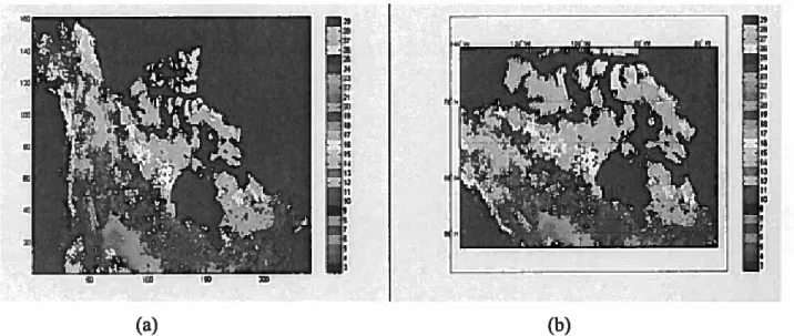
The estimation of sensible and latent heat fluxes typically requires knowledge of land cover charactedstics and surface states (Bertoldi et aI., 2008). Different land covers wilI have unique surface roughness and thermal characteristics, which affect the sensible and ground heat flux (Kampf and Taylor, 2006). In this part we used the “Land cover database of North America” for the year 2000. It is produced jointly by the Canada Centre for Remote Sensing (NRCan) and the US Geological Suiwey (Latifovic et al., 2002). It includes 29 classes (See Appendix B). In the present study, we will focus on 6 classes, as follows: 1-sub-polar mixed broadleaved or Needleleaved Forest,

2-G

k 2, 3, z 2, e t o N s n II t 4 I, I, w

Shrubland, 3-grassiand, 4-Cropland, 5-lichen and sparse vegetation, and 6-Water bodies.

We changed the resolution and projection on EASE-Grid for a resolution of 25 km. This way we were able to determine the percentage of classes for each pixel at 25 x 25 km (Kôhn, 2006). Figure 8 shows the resuits on the EASE-Grid projection.

_s F4’

I

• I, I,

I

II w

ii

Figure 8. Land cover classification ofNorth American year 2000 (Lafifovic et aI., 2002) (a) EASE-Grid projection and (b) visualization of the same figure in geographical

coordinates

5.1.5 Extraction of the NARR data

The wind components in x and y directions (U and V respectively), were acquired from the NARR at a 32 km resolution. After re-sampling and projected on EASE-Gdd (25 km), the wind speed (W) was calculated as follows (Holton, 2004):

W = (U2+ V2)”2 (7)

In addition to wind components, upward long radiation, downward long radiation upward short radiation , and downward short radiation are obtained from the NARR model at a 32 km resolution. After re-sampling and projected on EASE-Grid, net

20

radiation was calculated by relation (2). In order to compare the retrieved resuit with modelled; the sensible heat flux was extTacted.

The NARR air temperature (at 10 rn above ground) is used for the satellite-based retrieved sensible heat flux. It is assurned that this value depends pdrnarily on atmospheric conditions given by the model and then Ta is littie linked to the land cover (at the second order). It is then justified to use the NARR data (Ta, W,

5.2 Retrieval of sensible heat flux from satellite data

On the ground, sensible heat flux k typically determined from high frequency wind speed and air temperature measurements (eddy correlation technique). For remote sensing application, the sensible heat flux can be calculated based on the surface-air tcrnperature gradient and on aerodynamie resistance (Karnpfand Tyler, 2006).

The method of resistance is a combination method of energy balance, the relation between fluxes and gradients of mean quantities and an a priori evaluation of surface conditions. The general form is (Berkowice and Prahm, 1982):

Potential difference

FIux= . (8)

resistance

Depending on which quantity the flux refers to, the potential difference corresponds to the proper parameter. Thus, when the flux of heat is considered, the potential difference refers to temperature difference.

5.2.1 Retrieval of sensible heat flux

The sensible heat flux H (W/m2) can be deflned using the bulk resistance in a fashion analogous to Ohrn’s Law (Monteith, 1973). Figure 9 shows the schematic general form ofthe lheory:

H=pÇ

(9)

The regional distribution of sensible heat flux k expressed as follows (Ma and Ishikawa, 2003):

HG,y)=pÇ

7,y)—ï,,y)

surface temperature (°K) obtained from the SSMII, 7, is the air temperature (°K) obtained from the NARR model, ç is the aerodynamic resistance (snf’) determined by the Monin-Obukhov surface layer similarity theory, as follows:

çÇ,y)

=

kit

*

(x,y)

[ln(

Z—d0Ç,y)

_I+kB

_—,,G,y)

Z0,y)

Q

Where

k

is Von-Karman’s constant and its empirical constant with a value of about 0.40 (Hogstonn, 1985), while

u

* _{is the friction velocity (mis), expressed as follows (Ma and}

Ishikawa, 2003):

G

Reference height T, above eanopyr -T9

Figure 9. Schematic description of model for heat transfer (Source: Lia, 2004)

(10)

Where

p

is the air density(kgnï3),

C,,

is the specific heat of the air (Jkg’k’), ] is the

22

jjt,y) =kW,y) in[Z _do(xY) (ty)1 (12)

Z0,y) _j

Where Wft y) is the wind speed (mis) obtained relation (7). Z (Reference height = 10 m) is the height of the wind speed observed (StulI, 2000), Zo (t, j’,) k the aerodynamic

roughness length (m), roughness length is deflned by the logarithmic wind profile, and is valid in the lower part ofa neutrally stratified boundaiy layer (Dejong et al., 1999), and it is determined based on land cover classes. The value of Z0 depends on the characteristics of the surface (Sec Appendix 2) ranging from a value of 0.00 1 cm over smooth ice to 10 m over large buildings (Oke, 1978). d9is the zero-plane displacement height (m), which k proportional to the canopy height, as shown in the following (Quattrochi and LuvaIl, 2004):

d0fty) = 2/3 h,,(çy) (13)

where 1k is the canopy height (m), and is determined by the Eco-forestiy map. The

C)

added resistance term K’ = 2 (Garratt and Hicks, 1973), ift is a non-dimensional parameter, K& taking into account the flrndamental difference in the mechanisms determining heat and momentum transfer (Thom, 1972).

qi,, and çtçare the stability correction firnctions (dimensionless) for heat and

momentum transfers, respectively. The stability correction ffinctions are related to the stability condition of the atmosphere, which is characterized by the dimensionless Richardson number R (Businger, 1988):

Rftx,y)= 5• g(Z

—d0(x,y)1,Ç ,y) — Tjx,y))

(14)

;

(x)]+ 273.16]

where g is the acceleration due to gravity (mis2), Z is the reference height (m), d(t, y) the zero displacement height (m), Tsft y) the surface temperature (°K), Taft y)

atmosphedc temperature (°K), 11’(v, y) is the wind speed (mis). To detenEine correction

ftrnctions, we first calculated R (x, y).

Normal conditions exist when Ri = O, corrections fiinctions are as follows (StuIl 1998):

WmC’Y) = O and yi,,(.’çy) = 0.64 (15)

For unstable conditions (R<0), the stability correction ffinctions can be determined using the Businger-Dyer formulations (Businger, 1988; Sugita et al., 1990), which yield die following expressions:

m=2{1J+1{1t2att)+ (l

(1÷x2

çtç=2l9——

_I

(17)

©

For stable (R>0) conditions (Webb 1970)

(1

Where x=Q—16Ç)Zand(=(zr

—d)/L0,

in which L0 is the Obukhov stability length. 11e stability factor 4ean be replaced by the Richardson nutuber (Ri) using the following relationships (Thom, 1975; Businger, 1988):

Unstable

(19) Stable

I + 5

24 ____

Hftv) =çC,k2W(x,y) 7(x,y)—1(x,y) (20)

[i7_4-Y)]+

_WhCY)}[4 —G;Y)]mC’Y)

Z0(x,y)

_L

Z9Ç,y)

5.2.2 Estimation of Bowen Ratio

The energy balance equation (I) can be written as follows:

(x, y)— G (x, y) =L(x, y) ÷ H(x, y) (21)

Ground heat flux (G) is assumed negligible in Ibis study (mean daily budget), so the latent heat flux was retrieved as follows:

L(x, y) = R(x, y)— H(x, y) (22)

The partition of energy behveen sensible (H) and latent heat (L) flux is usually obtained by the Bowen ratio-energy balance method (Tanner et al., 1987; Kustas et al., 1996) by means ofthe Bowen ratio:

J3(x, y)= H(x, y)/ L(x, y) (23)

The Bowen ratio (j3) is a dimensionless quantity which measures the ratio of sensible to latent heat-flux densities and can be expressed as being proportional to the ratio of air temperature increment to vapor pressure increment over a finite height interval. Such a quantity is important to understand because knowledge of this variable quantifies the relative magnitudes of surface energy expenditure to heat the air and to evaporate water, and has been used widely in evaporation estimation (Revfeim and Jordan., 1976).

5.3 Temperature condition

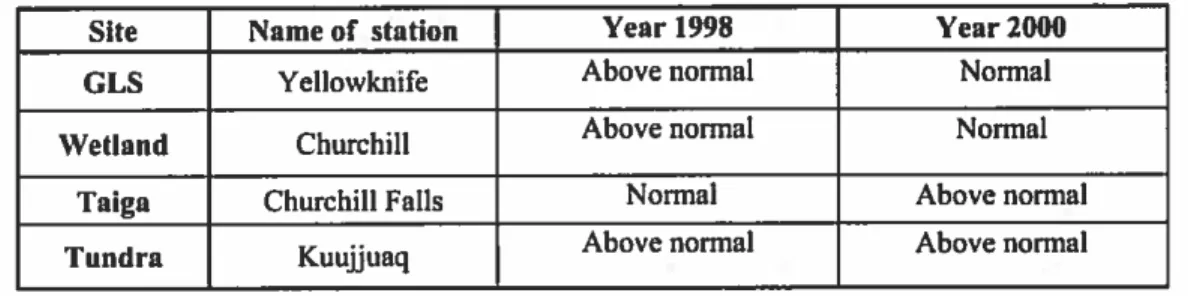
Atrnospheric temperatures of meteorological stations which were close to each site were considered as representative ofthe temperature conditions during the estirnated period. Table 3 shows the names of stations which are close to our study sites and the conditions for ifie two years considered as compared to the 197 1-2000 normaI (See Appendix 3).

Table 3. Name of sites and close meteorological stations

Site Name of station Vear 1998 Vear 2000

GLS Yellowknife Above normal Normal

Vetland Churchill Above normal Normal

Taiga ChurchillFalIs Normal Above normal

Tundra Kuujjuaq Above normal Above normal

6. Results

Ibis section presents the resuits of a concerted effort to compare the retrieved data on sensible heat at various sites in northem Canada with the resuits ofmodelling studies for the regions. The resuits from this study present a picture of the daily, rnonthly and seasonal behaviour of sensible energy over two summers (1998 and 2000) at the land-air interface.

6.1 Comparison behveen retrieved and modelled sensible heat flux

Figures 10, 11, 12, and 13 show the 3-dimensional variation of sensible heat flux as a function of FWS(% )and day in JuIy and August 1998-2000 for the GSL site. The rnodelled results show there are larger variations for less than 25% FWS and more than 70% FWS. However, when the FWS is between 25% and 70%, the modelled results indicate low variations. On the other hand, retrieved resuits show more variations of sensible heat flux for the range behveen 25% and 70%.

©

Sensible heat flwc( W1m2)

o

u, 0 0 00 00 w 0 o O o, O Sensible heat flux (W1m2) *

_ru

_n t n G

=

‘n O t’, G pz — o D -t, C 9:. -G ‘n C 5 z O E n D. n — I, “t— ‘t t’s ‘n *t’ D n © D C (t -t e D. n ci (t

r

‘n e n

z

I

O o, o w o e s Ce Q. _wt 0 (D (D w G,0 0 Mo o w o o0. C C 0. (0 t cc wo, M O O O o 3 oo o t’) ON o _{O o 3 o} ‘è

D

Sensible heat flux (W1m2) u, 0 00 0 0 0 0 0 *

_ru

_{p., n z z n} t I, n n z‘-t o z n

o

o

-è

z-

n

o z

z-o

Sensible heat flux (W/m2) u, o ô, u, 00 0 0 0 0 0 (no

ego

C -I (D

z.

(D

o-

t: t: -t t: e

o z o

-, rM (D

z

rd, D- (D

r

(D t: e t: r,, t:

z

n © z

o

-J Cl) -t e

r

(D C, Cl)

r

rM e (D

=

z

rM e C C C * -J 0 o, 0 w o :0 e e e u. _‘o ‘q M 0o 0 0 w o o oe e n. (n C‘q M 0o o M 0 o _o o 3 o w D o o M o w

na t o. (t R = SensIe heat lux (Whn2)

ul

:

H

!iil).h

DZ DZ

j

Sensible heat flux (W/mZ) La 3 o e

z -t (t

o

o

e

* _{rri n z z (t -t (t} t 1 o rM o z rn Q z n C Q z o Q z p-Sensible heat flux (Wdn2) o o D. et o -t C D C rM et D r,, et o o— o D n e © D C Ci) -t e D. et Ci)

r

rM e et z ze 9: e C eQ. C C M 0 0 0 £0 Sensible heeL flux (W/m2) — — 00 Cii O Cii 00 0 0 0 0 Cc

30

In order to evaluate the performance of the NARR model for different fraction values of water surfaces, we computed the retrieved and modelled sensible heat fluxes for the monthly mean and standard deviation against FWS during the summer months. Enor bars reflect the variance of sensible heat versus FWS for retrieved and modelled results.

For this purpose, we divided FWS into 5 equal intervals (1-20, 21-40, 41-60, 61-80, and 8 1-100% FWS). Then, monthly mean sensible heat fluxes and standard deviation for the pixels situated in each interval are calculated separately. Figure 14 shows the monthly mean of sensible heat versus FWS for the GSL site. It should be noted that for the GSL site in 2000, the month ofJune is incomplete. Because ofthe snow cover in the first half ofthe month, only the second halfwas processed.

For the GSL site, the two intervals (1-20% and 81-100% FWS) both resuits overlap (same mean values), meaning that there are no significant differences between the modelled and retrieved values for the area with no lake and the area covered with large lakes. On the other hand, for 20% < _FWS < _{80% values, there are fewer overlaps} between the modelled and retrieved enor bars. This indicates that there are more differences (in comparison) between the retrieved and modelled values over areas partially covered by water bodies.

Figure 15 shows the monthly mean of sensible heat versus FWS for the Wetland site. As the figure shows, for this site the modelled mean values are always higher (high negative values) than the retrieved satellite-based sensible heat flux (positive values). This could mean that the model does not take into account the land cover type. As a matter of fact, water bodies (small lakes and wetlands) remain wanner in August and September than the air. This Ieads to positive sensible heat flux for areas having high fraction of water surface. If the model does consider neither wetlands nor small lakes, it will calculate a high negative (downward) sensible heat flux, 50 the partition of sensible heat will be increased and the partition of latent heat decreased. On the other hand, the retrieved values which are based on high sensitivity to fracrional water surfaces show

ç’ C C o .4-’ t ce C’ o -c C u, t o ce o o o t u, o -o u, C o ‘n t— C C C .4-’ t ce C o -C 4-è et O -C o -o u, C O u, j O ce > z z O 8 ce E .2

I

* C ce z z o .2 Q u, t 2 t ce — .2 ce t Q -C Q — ce -o z ce Q z Q tE ce j-O Q -4-’ C o 4 .5 — Q C j-O CE -c E-* g g B B

}

(rwrA) nUII.q.I R R R

r

B 8

[Vi

9 4 8 E e R

I

‘D t O u, ce O s O C O -c 3 4-C O 4-ce

o

R w R R (zza% nJ èq aq...3 ‘z,A) nnu In.unqI,u.s R .t ..t’J.s

Q

o

o

SmnueI, xcix fi, (M,iQl Sensible noix flux wlmZ) M b à

o

SInI!bl. finI Ou, (Wrn2) C -t fit u’ et -t _1: et [M et z [M o. et z, et e C et -t [M C [M CM * et e z t z b * _{n n o -q, e n n n} pi, ou D, -t [M C- n p,e (D

I

s L s Sensible hast flux (VV1m2)

Ut

II Sensible heu flux W1m2) S,ns,bI. h.cl lii, b w t b g s s

I

Ut

k should be noted that for Wetland site, there are less variations of sensible heat flux versus FWS in comparison with the GSL site in the same period. Not only the retrieved results but also the modelled resuits show this pattem.

6.2 Emportance of lake size

In order to study the degree of importance of lake size in the variation of the sensible heat

flux, we considered cases with less than 20% FWS as a “No FWS” (NE), from 30-50% FWS

as a “Small EWS” (SF), from 50-80% FWS as a “Medium FWS” (MF), and from 80-100% as a “Large FWS” (LE).

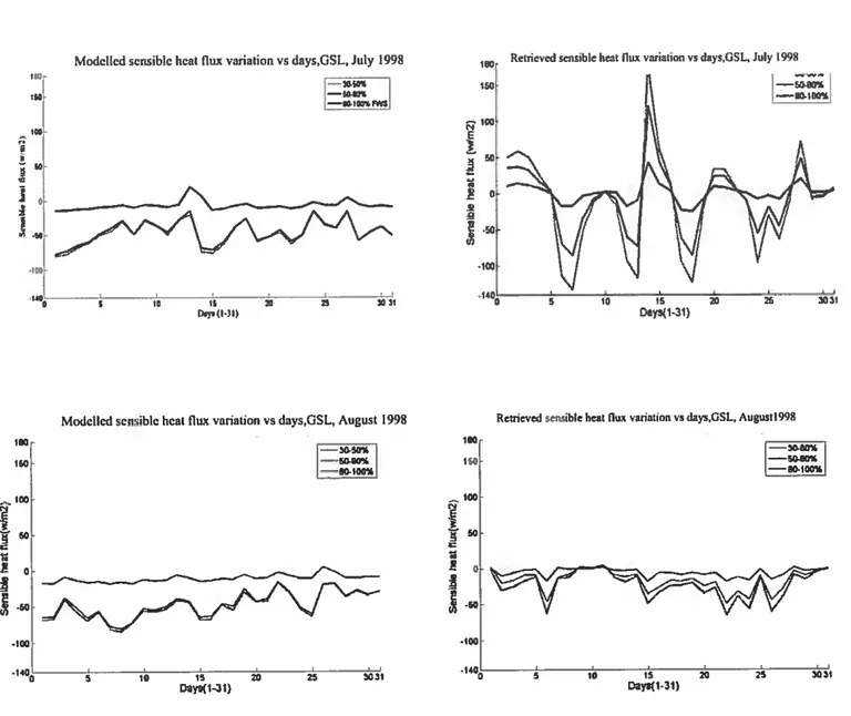
The daily average flux of sensible heat over these classes of fraction of water surface was estimated from retrievals and the NARR model. Figure 16 shows the daily values ofretrieved (right hand) and modelled (Ieft hand) sensible heat flux for three different classes, SF, ME and LE. As Figure 16 shows, the modelled sensible heat flux for the SE and ME are either very close or the same. However, for die retrieved flux, there are relatively more discrepancies between SF and MF classes.

In order to quantify these discrepancies, we used the Mean Absolute Enor (MAE) as sensible

heat flux measure difference between small FWS (SE) and medium FWS (MF).

1 ‘ci! cil

M4E= ZSHF-SHF (24)

IVtoiat i=i

where SHF and SHFt are the daily mean sensible heat flux values for the small EWS and medium FWS (ME) respectively. N,01, is the total number of days involved in the MAE. The derived MAE values are given in Table 4. The comparison of the retrieved MAE with the modeled MAE shows less sensibility ofthe model for small FWS and medium FWS.

34 550’ ‘sa 100 E ta 3 t. ! o, s .50[ o,’ ‘.0 ‘w 100 s t 10 -50

Figure 16. Daily values of sensible heat flux for separately, July and August 1998*

*Tle retHeved data are shown in the lefi and the modelled in the right hand.

GSL site for SL, ML and LL classes

Table 4. The MAE values (absolute difference behveen small and medium FWS) for modelled and

retrieved heat flux over July and August 1998

Resuit MAE (July 1998) MAE (August 1998)

Model 5.59 8.65

Retrieved 17.91 12.56

Modellcd sensible heat flux varialion vs days.GSL, Joly 1998

—n L’50’ rw:

Retrieved sensible hem flus variation vs days,GSL, JuIy 199g

-lot .100. l50f ‘t0

oh

_E E 5 10 15 3 -Days(1-31) 1 ‘0 il 20 20 5Oil [)ap(I-31)

ModelIed sensible heal flux variation vs days,GSL. AugusI 1998

—35n

5O-00

—50400%

Reffieved sensible hem flux variation vs days,GSL, AugustI99S

-—san —san 50-I00% .100 t 5 10 15 20 25 303’ 0 5 10 ‘5 20 25 3031 Days(1-31) Days(1-31)

6.3 Seasonal (monthly) sensible heat fluxes variation

In this part, surface-air temperature gradient (Ts-Ta) and monthly mean values of sensible heat fluxes versus FWS for the smdy sites were retrieved. Figures 17, 18, 19, and 20 show the surface-air temperature gradient and Lnonthly sensible heat flux variations for GSL and Tundra. As mentioned before for the GSL site in 2000, because of the snow cover, the month of June is incomplete. For the same reason, the graphs start with the month of July for the Tundra site.

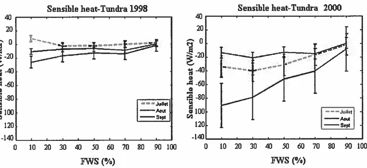
For the GSL and Tundra sites with an increasing FWS, surface-air temperature gradient and sensible heat flux magnitude typically decreases. In accordance with the increasing (decreasing) magnitude of surface-air temperature gradient, the partition of net radiation into sensible flux increased (decreased). Furthermore, we can say that when the FWS approaches 80-100%, the sensible heat values of the different months tend to overlap. Altematively, when the FWS is small (1-20%), the sensible heat values of different months are much more dispersed.

In general, at GSL (forested area), sensible heat decreases significantly from 460 W/m2 to 0-10 W1rn2. Over Tundra, the decreasing trend is less marked, from -20 W1m2 to O W1m2 (except for the rnonth of September 2000 where a significant increase is observed from -100 W/m2 to -10 W1m2).

Figures 21, 22, 23 and 24 show the pattems differ for the Wetland and Taiga sites. For the Wetland site, there is reverse variation; sensible heat is positive (+201+10 W/m2) for FWS<20%, and sensible heat flux varies between +10 and -10 W1m2 depending on the month. For the Taiga site, sensible heat flux is relatively constant when the FWS rises.

The year 2000 is representative of a normal summer, while the year 1998 was veiy warm (the warmest summer of the century). Both years, 1998 and 2000, show steeper surface-air temperature gradients and larger sensible heat flux magnitude for the month of Seplember, and the year 2000 presents the largest values for these two years.

36

Temperature gradient frends are different for 1998 and 2000. A warmer summer (1998, El Nino year) presents a smaller surface-air temperature gradient than summer 2000,

For the year 1998 in genemi, the seasonal heat flux for June and JuIy is aiways lower (O-20 W/rn2) than the end of the season (August and September), except for the Taiga site, where seasonally is not apparent.

Therefore, the observed variations of sensible heat versus the FWS depend on the land cover types surrounding the lakes, the summer months and the year considered.

As Figure 24 shows, there are inconsisteneies in the results between the Taiga site and the other sites, especially in the year 2000. For example, in 2000, the error bars for intervals 1-20% and 2 1-40% FWS show veiy close overlaps. On the other hand, for the inteivals 6 1-80% and 8 1-100%, there is less overlap. In 1998 the mean values versus the FWS are very close (see the mean values for intervals 1-20% and 80-100%). In section 6.4 we discuss more about the Taiga site.

In most cases, there are decreases in sensible heat with increasing FWS (except for the Taiga site). As a resuit, the inclusion of bodies of water in the undcrlying surface decreases the sensible heat flux.

—1 -2 -3 -4 -5 -6 20 -40 -80 100 3 2

co

E-4-1 E-L -3 -4 -5 -6 Ts-Ta-GSL 1998 3 2 0 Ts-Ta-GSI 2000 E-4 0 10 20 30 40 50 60 70 80 90 100

flVS

(%)

0 10 20 30 40 50 60 70 80 90100

flVS (%)

Figure 17. Average surface-air temperature gradient versus FWS% for four months (June, July, August, and September) in 1998 and 2000 for the GSL site

Sensible heat- GSL 1998

[

J20 n-60 Q 4) Sensible heat- GSL 2000 -100 —IIJl Jue1 —A —511’t 0 10 20 30 40 50 60 70 80 90 FWS (°/e) 0 10 20 30 40 50 60 70 80 90 100

Figure 18. Average sensible heat fluxes (retrieved) versus FWS% for four months (June, JuIy,

FWS (°,‘o)

38

Figure 19. Average surface-air temperature gradient versus FWS% for three months (July, August and September) in 1998 and 2000 for the Tundra

Figure 20. Average sensible heat fluxes (retrieved) versus FWS% for three months (JuIy, August and September) in 1998 and 2000 for the Tundra

e

Is-Ta-Tundra 1998

Is-Ta-Tundra 2000

3 2 c0 E-l-1 E-C .3 .4 .5 .6 --—JuIy ç—, —,

o

io

20 30 4850 60 70 80 90100

FWS

(%)

—StpI 3 2 E-l-1 b E-C .3 .4 .5 -6 40 20 ‘0 .4jJ o • -60 w -80 100 C., 120 -140 010203040 50 60 70 80 90 100

FWS (%)

Sensible heat-Tundra 1998 Sensible heat-Tundra 2000

———JutIIei —MiS —Sep 40 20 -40 o • -60 o 100 120 -140 0 10 20 30 40 50 60 70 80

o

100 FWS (%) —“ _Juillet —AoiS ——SepI 0 10 20 30 40 50 60 70 80 90 100 FWS

(%)

3 2 -3 -4 -5 -6 D 3 2 E-l-1 E-l -3 -4 -5 -6

Figure 21. Average surface-air temperature gradient versus FWS% for four months (June, July, August, and September) in 1998 and 2000 for the Wetland site

30 20

110

-c

k:

30 —20

L

-20 -30 10 10

Figure 22. Average sensible heat fluxes (retrieved) versus FWS% for four months (June, July, August, and September) in 1998 and 2000 for the Wetland site

o

Ts-Ta- Wetland 1998

Is-Ta- Wetland 2000

0102030405060708090100

FWS

(%)

0 10 20 30 40 50 60 70 20 90 100

FWS

(%)

Sensible heat-wedand 1998 Sensible heat-wetland 2000

—jwn Juillet — — FWS (%) o 10 20 30 40 50 60 70 80 90 100 FWS (%)

40

Figure 23. Average surface-air temperature gradient versus FWS% for four months

30 20

10

1M z o cil

(June, July, August, and September) in 1998 and 2000 for the Taiga site

(¾) 30 20

I

F0

-30 10 -20 -30 0 tO 20 30 4050 FWS

Figure 24. Average sensible heat fluxes (retrieved) versus FWS% for four months

10 0

Ts-Ta- Taiga 1998

3 2 co E-1-1 E-l -3 -4 -5 -6 Ts-Ta- Taiga 2000 I 3 2 E-1M’ E-4 -2 -3 -4 -5 -6 — — —sw1 0 10 20 30 40 50 60 70 80 90 100

flVS

(%)

10 20 30 40 50 60 70 80 90 100 FWS (°/o)

Sensible heat- Taiga 1998

— ——

—*o

—Sep

60 7080 90 1W

FWS /)

To better understand the spatial-temporal sensible heat variation, the energy balance relationships for the previously mentioned categories of FWS and for two different time intervals were calculated. The two time inteiwals were defined as follows:

1- First halfofthe summer: Early season (June lOto July 20). 2- Second haif ofthe summer: Late season (July 21 to August 30).

The (y/r) ratio was calculated for the two time intervals. The parameterx specifies the sensible energy balance component when there is less than 20% FWS (No FWS) and y is the sensible heat flux for the three different FWS classes (SF, MF, LF). This approach allows us to nomialize each site by their respective reference without lake that renders possibility the comparison between sites, having their own climate condition.

In order to determine the effect of different land type on sensible heat flux partition, the estimated and modelled ratios (y/r) are considered for 4 different sites. The early and late season periods have been distinguished. Figure 25 shows the ratio (y/x) for the GLS, Wetland, Taiga, and Tundra sites in 1998 and Figure 26 shows the ratio for 2000. The values of ratio are given for each site separately: Table 5. GSL; Table 6. Wetland; Table 7. Taiga; and Table 8. Tundra.

Figures 25 and 26 show the maximum retrieved ratios for the Taiga and Tundra sites and the minimum retrieved values for the GSL and Wetland sites. Such different results are mainly derived from the sites’ different land cover types. The predominant terrain type for the Tundra and Taiga sites is open mndra with less vegetation. This means that in these areas the greater part of the net radiant energy has to be converted into sensible heat and ground heat fluxes. Therefore, Figures 25 and 26 imply that the effects of lakes are closely related to the local setting of the lake and its surroundings. This is due to the difference in heat capacity, roughness length of water compared with nearby forest. In addition, Figures 25 and 26, just like the preceding results, show modelled ratios changed very little from one class of FWS to another, and suggests that the model is insensitive to the FWS in the interval 30-80%. Some examples are highlighted in green in Tables 5, 6, 7, and 8.

Retrieved ratio(y/x) for ail the sites-Early season 1998

42

Retrieved ratio(ylx) for ail the sites-bite season 1998

Modeiled ratio(ylx) for ail the sites-Eariy season 1998

o

Modelied ratio(y/x) for ail the sites-Ente season 1998

Figure 25. Comparison of the 4 sites- modelled and retrieved values over the

summer of 1998 5 4 3 2 I

n

H

5 4 3 2 I n

g

w Rcfricved GLS JjRefrieved WeUand JRcfrievedTaigaRefrievedTundra

.ri

__i

—1 -2 4 4 30-50% 50-80% 80-100% FWS% u ..

[JW

:.:.:îz.:.zzz.zz

g

w o 5 4 3 o -1 -2 -3 4 -5 30-50% 5030% 80-100% FWS% I ModeIIcdGSL LjModclledWeuand jJMcdcIIedTaiga -. ModellcdTurdra t o n 5 4 3 2 1

o

—1 -2 -3 4 -5 ModeIIedGSL

L

L

CModellcd WoUand ElMcdelledTaiga ModelledTundra 30-50% 5030% 80-100% 3040% 50-80% FWS% FWS% 80-I 00%

43

Retrieved ratjo(y/x) for ail the sites-Eariy season 2000 Retrieved ratiu(v/x) for ail the sites-Late season 2000

D 4 3

zzfrzzzzjIz

g

[:

_ni

j...

-2

!

•Refrieved E:JRefrieved WeUand 3 _{IjZJRefrievedTaip} 4 Hefrieved Tundra -5 I 3040% 50-80% 60-100% FWS%

Modelled ratjo(v/x) for ail the sites-Eariy seasun 2000 Modelied ratio(y/x) for ail the sites-Early season 2000

R j 5 4 3

g.

g.2

t

ti R ... .. x-i ModeIIedGSL -2 ..__ModeIIedWeUand -2 ModelledTundra 4

.

4 - I I 4 30-50% 50-60% 60-100% 3040% 5040% 60-100% FWS %

Figure 26. Comparison of the 4 sites- modelled and retrieved values over the

summer of 2000

3040% 5040% 60-100%

FW6%

ha

ihri in.

I....

. ModelIed

. I