arXiv:1105.4116v1 [astro-ph.IM] 20 May 2011
A Fast Algorithm for Muon Track Reconstruction and its Application to the
ANTARES Neutrino Telescope
J.A. Aguilara, I. Al Samaraib, A. Albertc, M. Andr´ed, M. Anghinolfie, G. Antonf, S. Anvarg, M. Ardidh, A.C. Assis Jesusi, T. Astraatmadja1i, J-J. Aubertb, R. Auerf, B. Baretj, S. Basak, M. Bazzottil,m, V. Bertinb, S. Biagil,m, C. Bigongiaria, C. Bogazzii, M. Bou-Caboh, M.C. Bouwhuisi, A.M. Brownb, J. Brunner2b, J. Bustob, F. Camarenah, A.
Caponen,o, C.Cˆarloganup, G. Carminatil,m, J. Carrb, S. Cecchinil,q, Ph. Charvisr, T. Chiarusil, M. Circellas, R. Coniglionev, H. Costantinie, N. Cottinit, P. Coyleb, C. Curtilb, M.P. Decowskii, I. Dekeyseru, A. Deschampsr, C. Distefanov, C. Donzaudj,w, D. Dornicb,a, Q. Dorostix, D. Drouhinc, T. Eberlf, U. Emanuelea, J-P. Ernenweinb, S.
Escoffierb, F. Fehrf, V. Flaminioy,z, U. Fritschf, J-L. Fudau, S. Galat`ab, P. Gayp, G. Giacomellil,m, J.P. G´omez-Gonz´aleza, K. Graff, G. Guillardaa, G. Halladjianb, G. Hallewellb, H. van Harenab, A.J. Heijboeri, Y. Hellor,
J.J. Hern´andez-Reya, B. Heroldf, J. H¨oßlf, C.C. Hsui, M. de Jong1i, M. Kadlerac, N. Kalantar-Nayestanakix, O. Kalekinf, A. Kappesf, U. Katzf, P. Kooijmani,ad,ae, C. Kopperf, A. Kouchnerj, V. Kulikovskiyaf,e, R. Lahmannf, P.
Lamareg, G. Larosah, D. Lef`evreu, G. Limi,ae, D. Lo Prestiag, H. Loehnerx, S. Loucatost, F. Lucarellin,o, S. Manganoa, M. Marcelink, A. Margiottal,m, J.A. Martinez-Morah, A. Mazurek, A. Melif, T. Montarulis,ah, M. Morgantiy,z, L. Moscosot,j, H. Motzf, C. Naumannt, M. Nefff, D. Palioselitisi, G.E.P˘av˘alas¸ai, P. Payreb, J. Petrovici, N. Picot-Clementeb, C. Picqt, V. Popaai, T. Pradieraa, E. Presanii, C. Raccac, C. Reedi, G. Riccobenev, C. Richardtf,
R. Richterf, A. Rostovtsevaj, M. Rujoiuai, G.V. Russoag, F. Salesaa, P. Sapienzav, F. Sch ¨ockf, J-P. Schullert, R. Shanidzef, F. Simeonen,o, A. Spiessf, M. Spuriol,m, J.J.M. Steijgeri, Th. Stolarczykt, M. Taiutie,ak, C. Tamburiniu, L. Tascak, S. Toscanoa, B. Vallaget, V. Van Elewyckj, G. Vannonit, M. Vecchin,b, P. Vernint, G. Wijnkeri, E. de Wolfi,ae,
H. Yepesa, D. Zaborovaj, J.D. Zornozaa, J. Z´u ˜nigaa
aIFIC - Instituto de F´ısica Corpuscular, Edificios Investigaci´on de Paterna, CSIC - Universitat de Val`encia, Apdo. de Correos 22085, 46071 Valencia, Spain
bCPPM - Centre de Physique des Particules de Marseille, Aix-Marseille Universit´e, CNRS/IN2P3, 163 Avenue de Luminy, Case 902, 13288 Marseille Cedex 9, France cGRPHE - Institut universitaire de technologie de Colmar, 34 rue du Grillenbreit BP 50568 - 68008 Colmar, France
dTechnical University of Catalonia,Laboratory of Applied Bioacoustics,Rambla Exposici´o,08800 Vilanova i la Geltr ´u,Barcelona, Spain eINFN - Sezione di Genova, Via Dodecaneso 33, 16146 Genova, Italy
fFriedrich-Alexander-Universit¨at Erlangen-N ¨urnberg, Erlangen Centre for Astroparticle Physics, Erwin-Rommel-Str. 1, 91058 Erlangen, Germany gDirection des Sciences de la Mati`ere - Institut de recherche sur les lois fondamentales de l’Univers - Service d’Electronique des D´etecteurs et d’Informatique, CEA
Saclay, 91191 Gif-sur-Yvette Cedex, France
hInstitut d’Investigaci´o per a la Gesti´o Integrada de Zones Costaneres (IGIC) - Universitat Polit`ecnica de Val`encia. C/ Paranimf 1. , 46730 Gandia, Spain. iNikhef, Science Park, Amsterdam, The Netherlands
jAPC - Laboratoire AstroParticule et Cosmologie, UMR 7164 (CNRS, Universit´e Paris 7 Diderot, CEA, Observatoire de Paris) 10, rue Alice Domon et L´eonie Duquet 75205 Paris Cedex 13, France
kLAM - Laboratoire d’Astrophysique de Marseille, P ˆole de l’ ´Etoile Site de Chˆateau-Gombert, rue Fr´ed´eric Joliot-Curie 38, 13388 Marseille Cedex 13, France lINFN - Sezione di Bologna, Viale Berti Pichat 6/2, 40127 Bologna, Italy
mDipartimento di Fisica dell’Universit`a, Viale Berti Pichat 6/2, 40127 Bologna, Italy nDipartimento di Fisica dell’Universit`a La Sapienza, P.le Aldo Moro 2, 00185 Roma, Italy
oINFN -Sezione di Roma, P.le Aldo Moro 2, 00185 Roma, Italy
pLaboratoire de Physique Corpusculaire, IN2P3-CNRS, Universit´e Blaise Pascal, Clermont-Ferrand, France qINAF-IASF, via P. Gobetti 101, 40129 Bologna, Italy
rG´eoazur - Universit´e de Nice Sophia-Antipolis, CNRS/INSU, IRD, Observatoire de la C ˆote d’Azur and Universit´e Pierre et Marie Curie, BP 48, 06235 Villefranche-sur-mer, France
sINFN - Sezione di Bari, Via E. Orabona 4, 70126 Bari, Italy
tDirection des Sciences de la Mati`ere - Institut de recherche sur les lois fondamentales de l’Univers - Service de Physique des Particules, CEA Saclay, 91191 Gif-sur-Yvette Cedex, France
uCOM - Centre d’Oc´eanologie de Marseille, CNRS/INSU et Universit´e de la M´editerran´ee, 163 Avenue de Luminy, Case 901, 13288 Marseille Cedex 9, France vINFN - Laboratori Nazionali del Sud (LNS), Via S. Sofia 62, 95123 Catania, Italy
wUniv Paris-Sud , 91405 Orsay Cedex, France
xKernfysisch Versneller Instituut (KVI), University of Groningen, Zernikelaan 25, 9747 AA Groningen, The Netherlands yDipartimento di Fisica dell’Universit`a, Largo B. Pontecorvo 3, 56127 Pisa, Italy
zINFN - Sezione di Pisa, Largo B. Pontecorvo 3, 56127 Pisa, Italy
aaIPHC-Institut Pluridisciplinaire Hubert Curien - Universit´e de Strasbourg et CNRS/IN2P3 23 rue du Loess, BP 28, 67037 Strasbourg Cedex 2, France abRoyal Netherlands Institute for Sea Research (NIOZ), Landsdiep 4,1797 SZ ’t Horntje (Texel), The Netherlands
acDr. Remeis Sternwarte Bamberg, Sternwartstrasse 7,Bamberg,Germany
adUniversiteit Utrecht, Faculteit Betawetenschappen, Princetonplein 5, 3584 CC Utrecht, The Netherlands aeUniversiteit van Amsterdam, Instituut voor Hoge-Energie Fysika, Science Park 105, 1098 XG Amsterdam, The Netherlands
afMoscow State University,Skobeltsyn Institute of Nuclear Physics,Leninskie gory, 119991 Moscow, Russia agDipartimento di Fisica ed Astronomia dell’Universit`a, Viale Andrea Doria 6, 95125 Catania, Italy
ahUniversity of Wisconsin - Madison, 53715, WI, USA
1Also at University of Leiden, the Netherlands
2On leave at DESY, Platanenallee 6, D-15738 Zeuthen, Germany
aiInstitute for Space Sciences, R-77125 Bucharest, M˘agurele, Romania
ajITEP - Institute for Theoretical and Experimental Physics, B. Cheremushkinskaya 25, 117218 Moscow, Russia akDipartimento di Fisica dell’Universit`a, Via Dodecaneso 33, 16146 Genova, Italy
Abstract
An algorithm is presented, that provides a fast and robust reconstruction of neutrino induced upward-going muons and a discrimination of these events from downward-going atmospheric muon background in data collected by the ANTARES neutrino telescope. The algorithm consists of a hit merging and hit selection procedure followed by fitting steps for a track hypothesis and a point-like light source. It is particularly well-suited for real time applications such as online monitoring and fast triggering of optical follow-up observations for multi-messenger studies. The performance of the algorithm is evaluated with Monte Carlo simulations and various distributions are compared with that obtained in ANTARES data.
1. Introduction
The main goal of neutrino telescope experiments such as AMANDA [1], IceCube [2], NT-200 in lake Baikal [3] and ANTARES [4] is the observation of high energy neutrinos from non-terrestrial sources. These instruments detect Cherenkov light from the passage of relativistic charged particles produced in neutrino interactions in the detector or its surrounding material. By measuring the photon arrival times at known positions, the particle trajectory can be re-constructed. The flight direction of these particles is nearly colinear with the incident neutrino direction for neutrinos above 10 TeV. The best angular resolution can be reached for νµ, ¯νµcharged current interactions where the measured particle is a muon that can travel several kilometres in water at TeV energies. Events induced by neutrinos from astrophysical sources must be distinguished from background which originates in the Earth’s atmosphere. Whereas atmospheric neutrinos are considered a non-reducible background (at least without the use of their energy), atmo-spheric muons can in principle be excluded by simple geometrical considerations. To exclude the contribution from downward-going atmospheric muons, it is sufficient to identify upward-going events, which can only be produced by neutrinos. This distinction requires a reliable determination of the elevation angle, because downward-going at-mospheric muons outnumber upward-going atat-mospheric neutrinos by 5 to 6 orders of magnitude for typical neutrino telescope installation depths.
In the following, a tracking algorithm is presented which meets this goal. Apart from providing an excellent up-down separation, it is very fast and therefore well-qualified for real time applications. This has been demonstrated in ANTARES, where the algorithm can cope with a trigger rate of 100 Hz, running on a single PC. It is used in various online monitoring tasks, for an analysis of atmospheric muons [5] and as an alert sending program to trigger optical follow-ups of selected neutrino events [6]. Other potential applications include the study of magnetic monopoles and nuclearites and the measurement of atmospheric neutrinos. The presented algorithm is complementary to other reconstruction methods which have been developped in ANTARES [7, 8].
Section 2 describes the ANTARES detector, Section 3 explains the geometrical approximations which are used in all subsequent steps. The hit merging and hit selection methods are detailed in Sections 4 and 5 whereas the fitting procedure can be found in Section 6. The performance of the entire algorithm introduced in Sections 2-6 is discussed in Section 7.
2. The ANTARES detector
The ANTARES detector is located about 40 km off the coast of Toulon, France, at a depth of 2475 m in the Mediterranean Sea (42◦48′N, 6◦10′E). It consists of 12 flexible lines, each with a total height of 450 m, separated by distances of 60-70 m from each other. They are anchored to the sea bed and kept near vertical by buoys at the top of the lines. Each line carries a total of 75 10-inch Hamamatsu photo multipliers (PMTs) housed in glass spheres, the optical modules (OM) [9], arranged in 25 storeys (three optical modules per storey) separated by 14.5 m, starting
100 m above the sea floor. Each PMT is oriented 45◦downward with respect to the vertical. A titanium cylinder in each storey houses the electronics for readout and control.
The positions of the line anchors on the sea bed and the construction details (cable length etc.) of each detector line are well known and stable in time. However the absolute positions and orientation of the individual OMs vary with time as the lines move freely in the sea current. Their movements are monitored by a system of acoustic transponders and receivers distributed over the lines and on the sea bed. After each cycle of acoustic signal exchange between these elements, a triangulation provides the shape of each line. This is complemented by data from a compass card within each electronics cylinder which measures the heading and the inclination of its storey. The processing of these combined data provides the position and orientation of each OM with a precision of better than 10 cm, but after an important delay.
3. Geometrical approximations
To qualify for real time applications the presented method uses only time independent geometrical informations and the following approximations are applied:
Line shape Detector lines are considered to be perfectly vertical. Line distortions due to sea currents are ignored. Storey geometry The detailed geometry of the storey is ignored. Each storey is considered as a single OM, which is
located directly on the detector line with an axis-symmetric field of view. The signals of the three PMTs within one storey are combined.
These approximations are used in the hit merging, hit selection and fitting steps. Their effect on the angular resolution is discussed in Section 7.3. Under the above approximations, a detector line is a straight line in space. It is also assumed that a muon track is a straight line, i.e. multiple scattering etc. is ignored. Except for the special case that the muon track and a detector line are parallel (in the case of an exactly vertical track), the point of closest approach of the muon track to the detector line can be determined. Most of the Cherenkov light is expected to be seen in the vicinity of this point. This is used in the hit selection as well as in the fitting procedure of the algorithm described below.
4. Hits and hit merging
The PMT signals are digitized by a custom built ASIC chip [10]. If the analog PMT signal crosses a preset threshold, typically 1/3 photoelectron (p.e.), its arrival time is measured together with its charge. The latter is obtained by integrating the analog PMT signal within a time window of 40 ns. Each such pair of time and charge is called a hit and the corresponding data for each hit are sent to shore. The data stream is processed by a computer farm in the shore station which searches for different physics signals according to predefined trigger conditions. If at least one trigger pattern is found, all hits within a time window of few µs around the trigger time are stored on disk. The DAQ system is described in detail in [11].
For the data which will be presented in Section 7.3 two trigger algorithms are used. Both rely on L1 hits which are defined either as 2 hits in coincidence within 20 ns in two OMs on the same storey or as a single hit with an amplitude larger than a threshold of 3 or 10 p.e.. One of the used triggers requires at least five causally connected L1 hits with respect to a given track direction. The second used trigger requires two pairs of L1 hits in adjacent or next-to-adjacent storeys within 80 ns and 160 ns respectively.
Before starting the actual hit selection, time and charge calibrations are applied to transform raw data to physical units such as time (in nanoseconds) and charge (in equivalent number of photoelectrons). Up to now the standard data handling in ANTARES has been described. The following steps are instead related to the presented algorithms. Different reconstruction methods might apply other hit treatment and hit selection procedures.
The calibrated hits are time-ordered for each storey. All hits on the same storey within a predefined time window are merged, as applied to early ANTARES data in [7]. Merging is performed by adding the hit charges and keeping the time of the earliest hit. The merging time window has to be chosen short enough to ensure a clean hit selection, with the earliest of the merged hits having a high probability of originating from a particle track. On the other hand,
the merging time window must be long enough to select most of the signal hits. For a 10-inch phototube, operated at a threshold of 0.3 photoelectrons a typical noise rate of 60-100 kHz is observed in sea water [12]. In this case a merging window of 20 ns is appropriate. As a result, a list of merged hits per storey is obtained and is the basis for all subsequent steps.
5. Hit selection
The light pattern expected from a highly relativistic charged particle is illustrated in Figure 1. The goal of the hit selection is to choose hits due to Cherenkov photons and avoid random hits from the optical background or scattered late hits. Late hits due to scattering are rare compared to typical optical background of 60-100 kHz. The probability of a Cherenkov photon at λ = 470 nm to suffer from light scattering on a path of 60 m (the inter-line distance and coincidentally the water absorption length) is only few per cent [13].
For tracks which are not parallel to a detector line, most of the Cherenkov light is expected near the point of closest approach of the track to the detector line. Therefore, the first step of the hit selection consists of finding a “hot spot” of light on a detector line which originates from Cherenkov light induced by a passing particle. In the presence of background light, a single high charge hit does not provide a “hot spot” with sufficient purity; two high charge hits in adjacent or next-to-adjacent storeys are needed. The detector storeys are numbered consecutively along the z-axis, like floors in a building. For a given floor i the adjacent or next-to-adjacent storeys are at floor i ± j with j = 1, 2. To ensure that hits on floors i and i ± j were caused by the same particle, the following condition on the absolute hit time difference ∆t is imposed
∆t < j∆zn
c+ ts, (1)
with ∆z the absolute vertical distance between adjacent storeys, c the speed of light in vacuum, n the refractive index of the medium and ts an additional time delay which accounts for the timing uncertainty of the photon detection
itself and the simplifications of the detector geometry. It is assumed that storeys are equally spaced. Such a causality condition has been used for hit selection prior to track reconstruction in Baikal [3] and AMANDA [14]. For the ANTARES detector with ∆z = 14.5 m and ts = 10 ns, one finds ∆t < 80 ns for adjacent and ∆t < 150 ns for
next-to-adjacent storeys. Only merged hits which originate from different PMTs or with a charge above 2.5 photoelectrons are considered here, because they have a high probability of being caused by a particle track. All hits which contribute to the above defined “hot spots” are stored as selected hits for the next steps. If several “hot spots” occur in the same storey at different times, only the earliest of them is kept.
For the following steps, only detector lines having at least one “hot spot” are considered. This condition removes all isolated hits from the sample. Using the “hot spot” hits as seeds, hits are added to the list of selected hits. From this point on, the hit selection is exclusively based on timing information. No charge cut is applied at this stage. This allows to use the attenuated signal at larger distances from the point of closest approach as illustrated in Figure 1. New hits on a given detector line are recursively sought within a narrow time window around the times of already selected hits. The expected hit times in adjacent or next-to-adjacent storeys are calculated, assuming the hits arrive linearly in the z-t plane as indicated by the asymptotes of the hyperbola in Figure 1. The projected arrival time ti± jat floor i ± j, ( j = 1, 2) is related to any pair out of the three hit times ti, ti∓1, ti∓2at floors i, i ∓ 1, i ∓ 2 in the following way
ti± j = ti+ j (ti− ti∓1), (2)
ti± j = ti+ j (ti− ti∓2)/2, (3)
ti± j = ti∓1+ ( j + 1) (ti∓1− ti∓2). (4)
In the following, time windows [tearlyi± j , tlate
i± j] based on the above equations are defined, which are used for the hit
selection. If only two out of the three hits in floors i, i ∓ 1, i ∓ 2 exist, only one of the extrapolations above can be performed. A new hit in floor i ± j is accepted if it occurred within a time window of
tearlyi± j = ti± j− jts (5)
tlatei± j = max(ti+ j∆z n
Time (ns) −1000 −500 0 500 1000 1500 Height (m) −200 −100 0 100 200 o 90 60o 30o 0o o 90 o 60 o 30 o 0 Time (ns) −1000 −500 0 500 1000 1500 Height (m) −200 −100 0 100 200 o 90 60o 30o 0o o 90 o 60 o 30 o 0
Figure 1: The pattern of Cherenkov light from a muon track; (left: upward-going; right: downward-going) on a single detector line. Vertical position (z-coordinate) along the detector line and photon arrival time are related by a hyperbola (see Equations 17,18). The point z = 0, t = 0 defines the point of closest approach between track and detector line; here, the track passes at 10 m. The colours correspond to different track
angles: black 90◦(vertical), red 60◦, green 30◦, blue 0◦(horizontal). The thickness of the lines indicates the brightness of the expected signal.
with ts and ∆z from Equation 1. This time window is asymmetric according to the generic shape of the Cherenkov
cone hyperbola in the z-t plane (see Figure 1 and Equations 17,18 discussed later). If all three hits exist, the minimum and maximum ti± jare determined and a time window of
tearlyi± j = ti± jmin− jts (7)
tlatei± j = ti± jmax+ jts, (8)
is used for floor i ± j. If several hits in floor i ± j meet the criteria, only the earliest one is selected. This procedure is applied recursively. If new hits cannot be found in either floor i ± 1 or i ± 2, the procedure stops, avoiding gaps of more than one floor. The occurrence of several well-separated “hot spots” on the same detector line serves as independent seeds to restart the procedure. The described hit selection is performed once. It yields at most one hit per storey. The result of the hit selection on a bright neutrino candidate event from 2008 can be seen in Figure 3.
6. Fitting procedure
Before starting any fit, the list of selected hits is examined. Only events with more than 5 hits are accepted. If all selected hits are on a single detector line, a procedure for a single-line fit is started, otherwise a multi-line fit procedure is performed. Both procedures are discussed in the following.
6.1. Fitting particle tracks
A particle track is considered to be a straight line in space. The particle is assumed to move with the speed of light in vacuum. All space-time points, ~p(t), that are part of the track can be parameterized as
~p(t) = ~q + c(t − t0)~u. (9)
The particle passes through the point ~q at time t0(i.e. ~q = ~p(t0)) and moves in the direction ~u. The vector ~q can be shifted along the track by redefining t0. Therefore the track is defined by a total of 5 parameters: three values to fix ~q for a given time and two angles to define ~u:
~u = {cos θ cos φ, cos θ sin φ, sin θ} , (10)
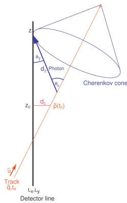
Detector line Track Cherenkov cone u q,to zc dc p(tc) Photon dγ z Lx,Ly θc θγ
Figure 2: Illustration of the variables used to describe a track and its corresponding Cherenkov cone with respect to a vertical detector line.
with θ the elevation angle and φ the azimuth angle. The detector lines are approximated as vertical lines along the z-axis (see Section 2) at fixed horizontal positions (Lx, Ly). The z-component of the point of closest approach of a particle track to a detector line is given by
zc=
qz− uz(~q · ~u) + uz(Lxux+ Lyuy)
1 − u2 z
, (11)
through which the particle passes at time tc= t0+ 1 c(Lxux+ Lyuy+ zcuz− ~q · ~u), (12) at a distance dc= q (px(tc) − Lx)2+ (py(tc) − Ly)2. (13)
The above-defined variables are illustrated in Figure 2. If the track is exactly vertical, and therefore parallel to the detector line, tc= t0and zc= qzare chosen. The track can be conveniently reparametrized in terms of zc, tc, dcfor each
detector line and the two angles which define ~u. For a single-line fit the detector line can be placed at the coordinate origin (Lx, Ly) = (0, 0) and Equations 11,12,13 simplify to
zc= qz− uz(~q · ~u) 1 − u2 z , (14) tc= t0+ qzuz− (~q · ~u) c(1 − u2 z) , (15) dc= q p2 x(tc) + p2y(tc). (16)
A single detector line is invariant against a rotation of the coordinate system around the z-axis. This means the track is not fully defined and only 4 parameters zc, tc, dcand uzcan be determined. No dependence from azimuth is observed.
To perform the track fit, it is necessary to know (a) the arrival time tγof a Cherenkov photon at the detector line positions (Lx, Ly, z), (b) its corresponding travel path dγand (c) its inclination with respect to the detector line, cos θγ. All three values can be derived from the parameters defined above and the refractive index n which is related to the Cherenkov angle θcby 1/n = cos θc:
tγ(z) = (tc− t0) + 1 c (z − zc)uz+ n2− 1 n dγ(z) ! , (17) dγ(z) = n √ n2− 1 q d2 c+ (z − zc)2(1 − u2z), (18) cos θγ(z) = (1 − u2z)z − z c dγ(z) + uz n. (19)
These equations hold exactly for Cherenkov photons of a given wavelength. Dispersion and group velocity effects as well as delays due to light scattering are ignored. An appropriate effective refractive index is used, depending on the medium in which the detector is installed.
6.2. Fitting point-like light sources: the bright-point fit
In contrast to a particle track, a ‘bright-point’ is defined as a point-like light source which emits a single light flash at a given moment. The light emission is assumed to be isotropic. The model of a bright-point does not only apply to artificial light sources such as optical beacons installed for detector calibrations [15] but also in some approximation to light from hadronic and electromagnetic showers, for which the actual extension of the shower is typically smaller than the detector line distances. A bright-point is defined by four parameters: its position ~q and its time t0. In analogy with the definitions of the point of closest approach for particle tracks, it is straightforward to see that for a bright-point zc= qz, tc= t0and dc= q (qx− Lx)2+ (qy− Ly)2, (20) which simplifies to dc= q q2 x+ q2y, (21)
for a single detector line at (Lx, Ly) = (0, 0). In this case, only the three parameters zc, tc, dccan be determined, which again means that the number of parameters is reduced by one. The photon arrival time tγ, its travel length dγand its angle with respect to a given arrival point z along the detector line can thus be determined in analogy to the case of a particle track: dγ(z) = q d2 c+ (z − qz)2, (22) tγ(z) = t0+ n cdγ, (23) cos θγ(z) = (z − q z) dγ . (24)
As in the treatment of particle tracks, it is assumed that all photons have the same wavelength, which corresponds to a fixed effective refractive index.
6.3. Quality function
The quality function is based on the time differences between the hit times ti and the expected arrival time tγ
of photons from the track or bright-point, as in a standard χ2 fit. The quality function is extended with a term that accounts for measured hit charges aiand the calculated photon travel distances dγ. The full quality function is
Q = Nhit X i=1 (tγ− ti)2 σ2 i +A(ai)D(dγ) haid0 , (25) 7
where hai is the average hit charge calculated from all hits which have been selected for the fit. The normalisation term d0and the functions A(ai) and D(dγ) are discussed below. The second term of the right hand side of equation 25
exploits the fact that an accumulation of storeys with high charges (hot spots) is expected on each detector line at its point of closest approach to the track. If such hot spots on several detector lines are arranged in a way that their z, t coordinates indicate an going pattern, the event has indeed a high probability to originate from an upward-going neutrino. This allows the isolation of a high purity neutrino sample. The concept is illustrated in Figure 3 where the arrangement of the “hot spots” on the various detector lines allows to classify this event as upward-going even without an overlaid fitted track. The quality function depends on a number of parameters which have been tuned for sea water [12, 13] and the ANTARES detector [4].
The timing uncertainty, σiis set to 10 ns for ai > 2.5 photoelectrons and to 20 ns otherwise. These values are
significantly larger than the intrinsic transit time spread of the ANTARES phototubes (1.3 ns). They take into account an additional smearing due to the applied geometrical approximations from Section 3 and due to the occasional presence of late hits from small angle scattering or from electromagnetic processes which passed the hit selection.
The charge term of the quality function is not arranged as a difference between expected value and measured charge in order to avoid incorrect penalties from large expected charges. Instead, the chosen form gives a heuristic penalty to the combination of high charge and large distance. The product is divided by the average charge of all the selected hits in an event, hai, to compensate for the fact that more energetic tracks or showers will produce more light at the same distance. The normalisation d0balances the weight between the two terms. For ANTARES a value of d0= 50 m has been chosen, motivated by the fact that at this distance the typical signal in a photodetection unit which points straight into the Cherenkov light front is of the order of one photoelectron.
The charges have to be corrected for the angular acceptance of the storey. Assuming a downward-looking hemi-spherical photodetection surface with a homogeneous efficiency for photodetection (a good approximation for an ANTARES storey), the following simple correction function for the hit charges a′
iis obtained: a′i = 2ai
cos θγ+ 1
. (26)
The average charge hai is calculated from these corrected hit charges:
hai = N1 hit Nhit X 1 a′i. (27)
Furthermore, charges are protected against extreme values by the following function: A(ai) = a0a′i q a2 0+ a′2i . (28)
The function A(ai) introduces an artificial saturation such that for a′i ≪ a0, the charge is relatively unaffected, i.e. A(ai) ≈ a′i, whereas for a′i≫ a0, the charge saturates at A(ai) ≈ a0, the chosen saturation value.
The photon travel distance is similarly protected using the function D(dγ) =
q d2
1+ d2γ, (29)
which introduces a minimal distance d1. For large distances, dγ ≫ d1, D(dγ) ≈ dγ, whereas for very small distances, dγ ≪ d1, D(dγ) ≈ d1. This avoids an excessive pull of the fitted trajectory towards the detector line.
Equations 28 and 29 can be motivated by the following consideration. The intensity of Cherenkov light decreases linearly with distance (ignoring absorption, dispersion and similar effects). Thus one can write a′idγ = a0d1. For ANTARES, the constant a0d1should be around 50 m×photoelectron, which corresponds to the observation that about 50 photoelectrons can be measured for a minimum ionizing particle at 1 m distance, or equivalently 1 photoelectron is seen at a distance of 50 m. Using this identity, it follows that A(ai)D(dγ) = a′idγ, i.e. the two functions have no effect
on the product of charge times distance for Cherenkov light; however, for background light they produce the desired penalty.
6.4. Minimization procedure
The MIGRAD function of the MINUIT package [16] is used to determine the minimum of the quality function Q. The value of Q/NDF (with NDF the number of degrees of freedom of the fit) after minimisation is called fit quality
˜
Q and is used for further selections. For the single-line bright-point fit, the parameters determined are the point of closest approach (i.e. zc, tc, dc) with an additional parameter uzin the case of a track fit. Equations 17-19 and 22-24
are used to obtain dγ, tγand cos θγfor particle tracks and bright-point fits, respectively.
The multi-line fits use the same set of equations. But in this case one more parameter is needed to evaluate them. For the multi-line track fit ~q, uzand φ are used, for the multi-line bright-point fit ~q and tc. Table 1 summarizes the
number of fit parameters for the different cases.
single-line multi-line
particle track 4 5
bright-point 3 4
Table 1: Number of parameters for the different fits. Since multi-line events do not have rotational symmetry, an additional parameter is required. A critical issue is the choice of the starting values and possible boundary conditions. As explained above, the set of fit parameters used for single-line bright-point fits is zc, tc, dc. Considering that most of the hits are grouped around the point of closest approach, zc ≈ hzii at tc ≈ htii, the mean values of the selected hit positions and times are used
as starting values. The initial choice of dcis not critical for the fit stability. It is set to dc = 10 m. This completely
determines the starting values for the single-line bright-point fit. For the single-line track-fit, a starting value for uz
has to be chosen as well. To avoid finding a wrong uz, due to the inherent ambiguities when fitting Cherenkov light
cones, three different starting values of uz are tried: −0.9, 0 and 0.9. The fit with the smallest fit quality ˜Q is taken.
The allowed parameter range for uzis limited to physical values (i.e. −1 ≤ uz ≤ 1). Fit results for which the fit stops
at a boundary are excluded.
The multi-line bright-point fit starts from the center of gravity of the selected hits in space and time. The multi-line track fit requires, however, a prefit. For this purpose, an improved version [8] of the “DUMAND prefit” [17] is used, which fits a straight line to the hit positions while allowing for a variable effective particle speed.
7. Test of the algorithm with Monte Carlo simulations and ANTARES data
The entire algorithm as described in Sections 3-6 was tested with ANTARES data and simulations of atmospheric muons and neutrinos.
7.1. Data sample
For the following analysis data are used which have been taken from December 2007 until end of 2008. During this time a minimum of 9 detector lines was active. From May 2008 on the ANTARES detector was complete with its 12 lines. Only runs are used, which have at least 80% of active channels when averaged over the run. A channel is called active if it has an instantaneous counting rate of at least 40 kHz, well below the typical baseline noise rate of 60 kHz. Further, runs are excluded for which more than 40% of the active channels have been in burst mode, which means they measure an instantaneous counting rate more than 20% above the usual baseline rate. This selection provides a data sample which corresponds to an active livetime of 173 days.
7.2. Simulations
Downward-going atmospheric muons were simulated with Corsika [18]. The primary flux was composed of several nuclei according to [19] and the QGSJET hadronic model [20] was used in the shower development. An average Mediterranean atmosphere is simulated, i.e. one which corresponds to a situation typically found in spring or autumn. Seasonal variations of the muon flux due to atmospheric temperature and density variations are found to be smaller than 3% in this region [21], and they are ignored in this analysis. Upward-going neutrinos were simulated according to the parameterization of the atmospheric νµflux from [22] in the energy range from 10 GeV to 10 PeV.
Only charged current interactions of νµand ¯νµwere considered. Disappearance of muon neutrinos due to neutrino oscillations was included in a simplified two-flavor model assuming maximal mixing and ∆m2= 2.4 · 10−3eV2.
The Cherenkov light, produced in the vicinity of the detector, was propagated taking into account light absorption and scattering in sea water [13]. The angular acceptance, quantum efficiency and other characteristics of the PMTs were taken from [9] and the overall geometry corresponded to the layout of the ANTARES detector [4]. The optical noise has been variable during the considered data taking period. It is simulated from counting rates observed in real data. At the same time the definition of active and inactive channels has been applied from real data runs of the selected period. The generated statistics corresponds to an equivalent observation time of 10 years for atmospheric neutrinos and, depending on primary cosmic ray energy, from 2 weeks up to 1 year for atmospheric muons.
A dedicated simulation has been done to study the impact of coincident atmospheric muon events. One month of equivalent livetime has been simulated using the MUPAGE code [23]. An increase of 0.1% is found at trigger level. The fraction of downward reconstructed tracks increases by a similar fraction whereas for misreconstructed upward-going tracks an increase of 0.2% is found without using a cut in the fit quality.
7.3. Results
The accuracy in the reconstruction of the elevation angle (the angle with respect to the horizontal plane), which needs to be good for up-down separation of the reconstructed tracks, is illustrated in Figure 4. The reconstructed elevation angle is plotted versus the true elevation angle for down-going atmospheric muons and upward-going at-mospheric neutrinos, that are reconstructed as multi-line events. No further event selection was applied. More than 95% of the fits converge for all events with selected hits on at least two lines. Most events are located within a narrow band around the diagonal and 80% of the events have their elevation angle reconstructed to better than 5◦. No other structures are visible on the plots. It should be noted that this excellent agreement is obtained, even though more than half of the triggered atmospheric muon events are muon bundles, whereas here just a single track reconstruction is performed.
Figure 5 confronts data and the two Monte Carlo samples for the full 173 days livetime. The left plot of Figure 5 shows the fit quality for the multi-line track fit of all the tracks reconstructed as upward-going. A cut on the track fit quality can effectively suppress background from misreconstructed atmospheric muons while maintaining a good efficiency for the atmospheric neutrino sample. A cut in the track fit quality of ˜Q < 1.4 ensures a 90% purity while keeping 48% of the total sample of upward reconstructed multi-line neutrino tracks. The cut selects 665 neutrino candidates in data (about 4 events per day), to be compared to 609 events from the atmopheric neutrino Monte Carlo sample and 40 misreconstructed downward-going atmospheric muon events. No event from the coincident muon sample survives the cut which gives a 90% upper limit of 13 such events in the final sample. Data and simulation agree within the shown statistical errors of the data for ˜Q < 1.4, whereas for ˜Q > 1.4 there is a systematic 30% excess of data. This excess is well within the estimated systematic error of the atmospheric muon simulation (see below). The resulting elevation angle distribution of the selected events with ˜Q < 1.4 is shown on the right plot of Figure 5. An excellent agreement between data and the atmospheric neutrino Monte Carlo sample based on the Bartol flux [22] is observed for the upward-going events, whereas the downward-going part features again a 30% excess of data with respect to the atmospheric muon simulation. The grey band gives the systematic error of the simulation. An extensive discussion of systematic effects is given in [5]. Main contributions are from the uncertainty in the effective area of the PMTs (10%), the uncertainty in the water absorption length (10%) and the uncertainty in the angular acceptance of the PMTs. The latter is better known close to the PMT axis (15% error) than in the backward hemisphere (up to 35% error) which leads to a larger total systematic error of 45% for downward-going atmospheric muons than for upward-going atmospheric neutrinos (32%). Within the quoted errors, data are compatible with the chosen flux models both for atmospheric neutrinos and for atmospheric muons.
Figure 6 compares data and simulation of some related quantities as the number of storeys used in the fit and the total charge of all hits used in the fit. Both plots show the comparison for the selected sample ˜Q < 1.4, which is dominated by atmospheric neutrinos. The shape of both distributions in data is well reproduced in the simulations.
Figure 7 shows the effective area for all reconstructed multi-line events as function of the true neutrino energy. The comparison of the solid and the dotted line indicates that more than 40% of the events pass the quality cut of ˜Q < 1.4 for energies below 10 TeV. This fraction reduces to 20% at 100 TeV and decreases further for higher energies. The low efficiency at highest energy can be explained by the use of a quality cut, which has been derived from Figure 5 for
Zenith : 27.2 Fit on 8 line(s) time (nsec) −1000 −500 0 500 1000 1500 2000 height (m) 0 50 100 150 200 250 300 350 400 450 500 Line 1 time (nsec) −1000 −500 0 500 1000 1500 2000 height (m) 0 50 100 150 200 250 300 350 400 450 500 Line 2 Run 37246 Frame 44741
Wed Nov 19 05:28:37 2008 UTC
Trigger bits 80002020 Line 1−12 Physics Trigger − Noisy channels treated
1 2 3 4 5 6 photons time (nsec) −1000 −500 0 500 1000 1500 2000 height (m) 0 50 100 150 200 250 300 350 400 450 500 Line 5 time (nsec) −1000 −500 0 500 1000 1500 2000 height (m) 0 50 100 150 200 250 300 350 400 450 500 Line 3 time (nsec) −1000 −500 0 500 1000 1500 2000 height (m) 0 50 100 150 200 250 300 350 400 450 500 Line 4 time (nsec) −1000 −500 0 500 1000 1500 2000 height (m) 0 50 100 150 200 250 300 350 400 450 500 Line 6 time (nsec) −1000 −500 0 500 1000 1500 2000 height (m) 0 50 100 150 200 250 300 350 400 450 500 Line 9 time (nsec) −1000 −500 0 500 1000 1500 2000 height (m) 0 50 100 150 200 250 300 350 400 450 500 Line 7 time (nsec) −1000 −500 0 500 1000 1500 2000 height (m) 0 50 100 150 200 250 300 350 400 450 500 Line 8 time (nsec) −1000 −500 0 500 1000 1500 2000 height (m) 0 50 100 150 200 250 300 350 400 450 500 Line 10 time (nsec) −1000 −500 0 500 1000 1500 2000 height (m) 0 50 100 150 200 250 300 350 400 450 500 Line 11 time (nsec) −1000 −500 0 500 1000 1500 2000 height (m) 0 50 100 150 200 250 300 350 400 450 500 Line 12
Figure 3: Event display of a bright neutrino event from the 2008 data taking period. The arrangement of the 12 histograms corresponds approxi-mately to the octagonal layout of the 12 detector lines on the sea floor. For each line the vertical position above the sea floor (m) is given as function of the hit time (ns) (see also Figure 1). t = 0 corresponds to the time of the first hit which participated in the trigger. A window of −1000/ + 2000 ns is shown with respect to this time. z = 0 indicates the sea floor. Active detector elements are between z = 100 and z = 450 m. Circles denote hits which participated in the trigger, crosses are other hits, boxes indicate the hit selection of Section 5. Colors refer to the hit charge as shown in the legend on the top right part of the figure. The line width and style of the fitted track illustrates the minimal distance between track and detector line; thick and solid lines stand for closer distances than thin or dotted lines.
MC θ sin 0.4 0.5 0.6 0.7 0.8 0.9 1 Reco θ sin 0.4 0.5 0.6 0.7 0.8 0.9 1 5000 10000 15000 20000 25000 30000 35000 40000 45000 MC θ sin −1 −0.9 −0.8 −0.7 −0.6 −0.5 −0.4 −0.3 −0.2 −0.1 0 Reco θ sin −1 −0.9 −0.8 −0.7 −0.6 −0.5 −0.4 −0.3 −0.2 −0.1 0 0 0.2 0.4 0.6 0.8 1 1.2 1.4 1.6
Figure 4: Correlation between reconstructed and simulated elevation angle; Left: down-going atmospheric muon events; Right: upward-going atmospheric neutrino events.
Track Fit Quality
0 0.5 1 1.5 2 2.5 3 Number of events 1 10 2 10 3 10 4 10 Reco θ sin −1 −0.8 −0.6 −0.4 −0.2 0 0.2 0.4 0.6 0.8 1 Number of events 1 10 2 10 3 10 4 10 5 10 6 10
Figure 5: Left: track fit quality for all upward reconstructed multi-line tracks for 2008 data (points with error bars) compared to a Monte Carlo sample of downward-going atmospheric muons (dashed histogram) and upward-going atmospheric neutrinos (solid histogram); right: Elevation
angle distribution for events with ˜Q < 1.4. The grey band indicates the error band of the combined prediction from neutrino and muon simulations.
Number of Storeys 5 10 15 20 25 30 35 40 Number of events −1 10 1 10 2 10 Amplitude (p.e.) 50 100 150 200 250 300 350 400 Number of events −1 10 1 10
Figure 6: Left: Number of storeys and Right: total charge used in the track fit for all upward reconstructed multi-line tracks for events with ˜
Q < 1.4. Data (points with error bars) are compared to a Monte Carlo sample of downward-going atmospheric muons (dashed histogram) and
) ν (E 10 log 1 2 3 4 5 6 7 ) 2 (m eff A −6 10 −5 10 −4 10 −3 10 −2 10 −1 10 1 10
Figure 7: Effective area for all multi-line events (solid), selected events with ˜Q < 1.4 (dotted) and selected events with ˜Q < 1.3 + (0.04 · NDF)2
(dashed) as function of the true neutrino energy for upward-going neutrinos.
atmospheric neutrinos. By modifying the selection criteria one can easily recover the high energy part. The condition ˜
Q < 1.3 + (0.04 · NDF)2 is used for the dashed line. It has the same performance as ˜Q < 1.4 for E
ν < 10 TeV where atmospheric neutrinos dominate, but a much improved performance at Eν > 10 TeV. NDF = Nstorey− 5 is here used as a simple estimator for the brightness and therefore energy of an event. This modified cut selects 624 events in data to be compared to 588 atmopheric neutrinos and 40 atmospheric muons keeping the quoted 90% purity of the neutrino sample. A full likelihood fit [8] has a similar performance at high energies when requiring a 90% purity for atmospheric neutrinos. For energies below 1 TeV the method presented here is found more efficient than the likelihood fit.
| Reco θ − MC θ | 0 1 2 3 4 5 6 7 8 9 10
Number of events (a.u.)
0.005 0.01 0.015 0.02 0.025 0.03 0.035 0.04 0.045 0.05 ) data u • MC u acos( 0 2 4 6 8 10
Number of events (a.u.)
0.0005 0.001 0.0015 0.002 0.0025 0.003 0.0035 0.004
Figure 8: The distributions, normalized to the same content, of the angular error in degrees for selected atmospheric neutrinos (full) and atmospheric muons (hatched); left: elevation angle error for multi-line events; right: space angle error for non-coplanar hit selection.
Figure 8 shows the angular resolution of the data sample which is selected by a cut of 1.4 on the fit quality. Both plots of Figure 8 are integrated over the full angular range and over the atmospheric neutrino energy spectrum. The elevation angle is reconstructed with a precision of 0.4◦for upward-going neutrino-induced muons and 0.5◦for down-going muons (median of the angular error compared to the true muon direction). The space angle can only be unambiguously defined if the selected hits do not lie in a plane. Mirror solutions in azimuth are otherwise unavoidable. Because of the simplifications of the detector geometry used during reconstruction, a non-coplanar hit selection can only be achieved when hits from at least three detector lines are used. This condition is fulfilled for 25% of the
selected multi-line atmospheric neutrino events. For this sub-sample a median space angle error of 1.0◦is found for atmospheric neutrinos and 1.4◦for atmospheric muons as shown on the right plot of Figure 8.
7.4. Improving the angular resolution
The angular resolution which has been quoted in the previous section can be improved in several ways, without changing the event selection and without compromizing the speed of the algorithm.
Resolving azimuthal degeneracy
For a particle trajectory reconstructed using hits on only two straight detector lines, there always exists an alterna-tive trajectory having an identical ˜Q-value, but a different direction. The two trajectories will have the same elevations, but will differ in their azimuthal orientation. The degenerate trajectory is easily determined given the positions of the two detector lines and the trajectory resulting from the fit. First, the point at which the particle trajectory crosses the plane connecting the two detector lines is determined. The trajectory is then rotated about this point by an angle 2ψ to form the degenerate track candidate, where ψ is the angle between the fit result and the plane connecting the two detector lines.
Armed with both possible track solutions, the two candidates can be discriminated with the following procedure. The time residuals of all hits are calculated from the differences of the actual hit times and the theoretical hit times according to Equation 17. The sum of the charge of each hit having a time residual smaller than 30 ns is then calculated. This can include hits from any line and not just the two used in the original fit, helping to break the degeneracy. The hit selection is done separately for both track candidates and the candidate with the largest total charge is chosen. In simulations of both downward-going muons and upward-going neutrinos this procedure chooses the correct track candidate 70% of the time and improves the two-line angular resolution by 42% for upward-going atmospheric neutrinos and by 15% for downward-going atmospheric muons.
Additional fit step
Taking the result of a multi-line track fit or its mirror solution as it was described in the previous sections as a prefit, a new hit selection and a subsequent fit is performed. Every hit which has a time residual smaller than 20 ns with respect to the prefit track is chosen. These hits are then used to minimize the function
M = Nhit X i=1 2 s 1 + (tγ− ti) 2 2σ2 − 2 , (30)
which is a robust estimator that combines the properties of both least-squares and absolute-value minimizers [24]. This estimator is quadratic for small values of the time residual (i.e. when |tγ− ti|/σ ≪ 1), just as with a standard χ2estimator, but is linear for large time residuals. It is therefore not affected as dramatically by background hits with large residuals surviving the hit selection. Note that only the time residual of hits are minimized at this stage; no information concerning the number of photoelectrons detected is used. For the current studies σ = 1 ns has been taken. The precise value of σ has little impact on the angular resolution.
Use of the detailed detector geometry
While the algorithm has so far assumed a simplified detector geometry, it is possible to extend it in order to exploit the actual location and orientation of the PMTs. This detailed geometry information can be employed in the calculation of the predicted photon arrival time (tγin Equation 30). The use of the resulting time residual for both the hit selection and track fit minimization, as described in the previous section, has been studied. Simulations for this study have been performed in the absence of sea currents, i.e. again for straight detector lines. The systematic angular shift due to the coherent inclination of all detector lines in a horizontal sea current is estimated to be smaller than 0.2◦ for a typical sea current of 5 cm/s as measured at the ANTARES site. However, such a systematic shift is not included in the numbers and figures quoted below.
Results
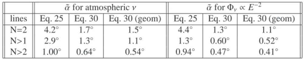
The effect of these three additional steps can be seen in Table 2, which compares the median angular error of the multi-line algorithm described in Section 6.1 to the subsequent fit using Equation 30 with and without the use of a detailed detector geometry. The condition on the number of detector lines N, from which hits have been used in the fit, is specified in the first column of Table 2. Results are given for upward-going atmospheric neutrinos as well as for neutrinos from an E−2ν flux, which is typical for astrophysical sources. Only events which fulfill the condition
˜
Q < 1.3 + (0.04 · NDF)2are included.
For tracks reconstructed using hits on only two lines in the initial fit, the improvement can be attributed mainly to the partial resolution of the azimuthal symmetry. For the case where more than two lines had been used initially, the main improvement comes from the additional fit step. An additional 0.1◦in resolution may be gained by using the detailed detector geometry within each storey. The full multi-line sample (N > 1) profits from a combination of both effects.
˜
α for atmospheric ν α for Φ˜ ν∝ E−2
lines Eq. 25 Eq. 30 Eq. 30 (geom) Eq. 25 Eq. 30 Eq. 30 (geom)
N=2 4.2◦ 1.7◦ 1.5◦ 4.4◦ 1.3◦ 1.1◦
N>1 2.9◦ 1.3◦ 1.1◦ 1.3◦ 0.60◦ 0.52◦
N>2 1.00◦ 0.64◦ 0.54◦ 0.94◦ 0.47◦ 0.41◦
Table 2: The median angular error ( ˜α) in the multi-line fit algorithm as of Section 6.1 and the subsequent fit with and without using geometry
information, for atmospheric neutrinos and neutrinos from an E−2flux.
The improvement in the angular error for neutrino-induced muons can also be seen in Figure 9 (left), which shows the energy dependence of the median angular deviation from the true muon direction for all reconstructed tracks using hits on more than 2 lines having a ˜Q-value better than 1.3 + (0.04 · NDF)2. The selection is applied only to the original track fit, so that the observed improvement of the angular resolution is the result a refined hit selection, combined with a new fit. The three curves correspond to the multi-line track fit from Section 6.1 (solid) and the fits using Equation 30 with an approximated geometry (dotted) and with a detailed geometry of each storey (dashed). The muon track angular error is almost energy independent at neutrino energies above 10 TeV. It converges to the values quoted in table 2 for an E−2flux.
This can be compared to the performance of a full likelihood fit [8] which uses the full geometry, a detailed modelling of the time residual, (e.g. an energy dependent tail of late hits and a contribution of noise hits) and which applies a scan of starting positions of the fit to avoid local minima. Such a procedure can reach an angular resolution of 0.3◦at high energies for the entire multi-line sample, while using about 10 times more computing time than the method presented here.
Figure 9 (right) shows the point spread function for neutrino events after the fit from Equation 30. Contrary to the figures shown earlier the angular error is given here with respect to the neutrino direction - a quantity which is relevant to point back to a potential neutrino source. The optical followup program [6] uses a sub-sample of the events, shown on the dashed line in Figure 9 (right). As the field of view of the used robotic telescope is of the order of 2◦, it can be seen that more than 70% of the candidate sources would lay inside the field of view.
The improvement is further demonstrated by the time residual distributions, as shown in Figure 10. The time residuals are shown for all hits in each event for atmospheric neutrino events. The residuals of the subsequent fit using the detailed geometry show a more pronounced peak at zero, whose width is roughly 40% smaller compared to the multi-line fit from Section 6.1.
These extensions to the algorithm do not significantly affect the time needed for track reconstruction. Including the subsequent fit, the entire reconstruction algorithm takes an average of 5 ms per muon event on an Intel Xeon 2.66 GHz CPU for events recorded by the 12-line ANTARES detector.
8. Conclusions
A generic and fast track fit algorithm for muon tracks in neutrino telescopes has been presented which can reliably distinguish upward-going neutrinos from the overwhelming background of downward-going muons. The method is
(GeV) ν E 10 Log 1 2 3 4 5 6 (deg) α∼ 0 0.2 0.4 0.6 0.8 1 1.2 1.4 1.6 1.8 2
Angular error (degree)
0 0.5 1 1.5 2 2.5 3 3.5 4 4.5 5 Fraction of events 0 0.1 0.2 0.3 0.4 0.5 0.6 0.7 0.8 0.9 1
Figure 9: Left: Dependence of the angular resolution for selected tracks ( ˜Q < 1.3 + (0.04 · NDF)2, N > 2) on Eν. The median angular error
of the multi-line fit (solid line) is compared against the fit from Equation 30 without (dotted) and with (dashed) use of a detailed description of
the geometry of a storey; right: Cumulative point spread function for selected upward-going neutrino events with an E−2spectrum and ˜Q <
1.3 + (0.04 · NDF)2, N > 2 for multi-line fits (solid) and fits from Equation 30 with an approximate geometry (dotted).
used in ANTARES for different applications such as an online event display, a neutrino monitor and an alert sending program to trigger optical follow-ups of selected neutrino events. It has also been used for an analysis of atmospheric muons [5]. Other potential applications include the study of magnetic monopoles and nuclearites and the measurement of atmospheric neutrinos.
9. Acknowledgement
The authors acknowledge the financial support of the funding agencies: Centre National de la Recherche Sci-entifique (CNRS), Commissariat `a l’Energie Atomique et aux Energies Alternatives (CEA), Agence National de la Recherche (ANR), Commission Europenne (FEDER fund and Marie Curie Program), R´egion Alsace (contrat CPER), R´egion Provence-Alpes-Cte d’Azur, D´epartement du Var and Ville de La Seyne-sur-Mer, France; Bundesministerium f¨ur Bildung und Forschung (BMBF), Germany; Istituto Nazionale di Fisica Nucleare (INFN), Italy; Stichting voor Fundamenteel Onderzoek der Materie (FOM), Nederlandse organisatie voor Wetenschappelijk Onderzoek (NWO), the Netherlands; Council of the President of the Russian Federation for young scientists and leading scientific schools supporting grants, Russia; National Authority for Scientific Research (ANCS), Romania; Ministerio de Ciencia e In-novaci´on (MICINN), Prometeo of Generalitat Valenciana and MultiDark, Spain. Technical support of Ifremer, AIM and Foselev Marine for the sea operation and the CC-IN2P3 for the computing facilities is acknowledged.
References
[1] J. Ahrens et al. [AMANDA Collaboration], Astrophys. J. 583 (2003) 1040. [2] R. Abbasi et al. [IceCube Collaboration], Astrophys. J. 701 (2009) 47. [3] V. A. Balkanov et al. [Baikal Collaboration], Astropart. Phys. 12 (1999) 75. [4] M. Ageron et al. [ANTARES Collaboration], Astropart. Phys. 31 (2009) 277. [5] J.A. Aguilar et al., [ANTARES Collaboration], Astropart. Phys. 34 (2010) 179. [6] D. Dornic et al., arXiv:0810.1416 [astro-ph].
[7] R. Bruijn, PhD thesis, University of Amsterdam, March 2008.
(http://www.nikhef.nl/pub/services/biblio/theses_pdf/thesis_R_Bruijn.pdf ) [8] A. Heijboer, PhD thesis, University of Amsterdam, June 2004, p.57ff.
(http://www.nikhef.nl/pub/services/biblio/theses_pdf/thesis_A_Heijboer.pdf ) [9] P. Amram et al., [ANTARES Collaboration], Nucl. Instrum. Meth. A 484 (2002) 369.
(ns) pred - t hit t -30 -20 -10 0 10 20 30
Number of hits (a.u.)
-7 10
-6 10
Figure 10: Time residuals of all hits (not just those used in the fit) for the multi-line track fit (full) and the subsequent fit using geometry information (hatched).
[11] J.A. Aguilar et al., [ANTARES Collaboration], Nucl. Instrum. Meth. A 570 (2007) 107. [12] P. Amram et al., [ANTARES Collaboration], Astropart. Phys. 13 (2000) 127.
[13] J.A. Aguilar et al., [ANTARES Collaboration], Astropart. Phys. 23 (2005) 131. [14] J. Ahrens et al. [AMANDA Collaboration], Nucl. Instrum. Meth. A 524 (2004) 169. [15] M. Ageron et al., [ANTARES Collaboration], Nucl. Instrum. Meth. A 578 (2007) 498. [16] F. James and M. Roos, Comput. Phys. Commun. 10 (1975) 343.
[17] V. Stenger, DUMAND External report HDC-1-90, 1990.
[18] D. Heck et al., Report FZKA 6019 (1998), Forschungszentrum Karlsruhe; D. Heck and J. Knapp, Report FZKA 6097 (1998), Forschungszentrum Karlsruhe. [19] S.I. Nikolsky et al., Sov. Phys. JETP 60 (1984) 10;
E.V. Bugaev et al., Phys. Rev. D58 (1998) 05401.
[20] N.N. Kalmykov and S.S. Ostapchenko, Yad. Fiz. 56 (1993) 105; N.N. Kalmykov and S.S. Ostapchenko Phys. At. Nucl. 56(3) (1993) 346. [21] M. Ambrosio et al., [MACRO Collaboration], Astropart. Phys. 7 (1997) 109;
Y. Becherini et al., [MACRO Collaboration], Astropart. Phys. 23 (2005) 341.
[22] G. Barr et al., Phys. Rev. D39 (1989) 3532; V. Agrawal et al., Phys. Rev. D53 (1996) 1314. [23] G. Carminati et al., Comput. Phys. Commun. 179 (2008) 915.
[24] Z. Zhang, Image and Vision Computing Journal 15 (1997) 59.