Élasticité de la demande d'autoroutes à péage au Mexique = : Demand elasticity for Mexican toll roads

MARCO ANTONIO LOPEZ CASTRO

ELASTICITE DE LA DEMANDE D'AUTOROUTES

À PÉAGE AU MEXIQUE

Demand Elasticity for Mexican Toll Roads

Mémoire présenté

à la Faculté des études supérieures et postdoctorales de l'Université Laval dans le cadre du programme de maîtrise en économique

pour l'obtention du grade de Maître es arts (M.A.)

DEPARTEMENT D'ECONOMIQUE FACULTÉ DES SCIENCES SOCIALES

UNIVERSITÉ LAVAL QUÉBEC

2012

Résumé

Cette étude cherche à estimer l'élasticité-prix de la demande pour les segments du principal réseau d'autoroutes payantes du Mexique ainsi que d'établir quels sont les facteurs qui déterminent sa magnitude. L'expérience mexicaine sur la concession d'autoroutes illustre le risque d'ignorer la sensibilité de la demande au péage. L'élasticité-prix est estimée en utilisant une analyse de régression sur des données de type panel. Les résultats indiquent que les usagers des autoroutes payantes du Mexique sont plus sensibles aux variations des prix qu'on s'y serait attendu. En outre, la valeur absolue de l'élasticité-prix à court terme diminue selon la longueur du segment routier et selon la proportion de camions lourds dans les voix alternatives. Ce résultat pourrait impliquer que la sensibilité aux variations du péage diminue quand les économies potentielles de temps augmentent et la dégradation des routes alternatives due au trafic lourd accroît.

11

Abstract

The objective of this study is twofold. First, to provide price demand elasticity estimates for each road segment of Mexico's largest tolled motorway network. Second, to establish which factors can explain the variation of these estimates. Unawareness about the users' sensitivity to toll variations can lead to crucial mistakes as has already happened during Mexico's first road concession program. We estimate toll elasticities for each road segment using a panel data regression approach. Our results show that on average Mexican toll road users are more sensitive to tariff variations than usually expected. Furthermore, the absolute value of the short term elasticity decreases with the toll road segment length and with the freeway's proportion of heavy traffic. This could indicate that toll road users become less sensitive to tariff changes as time savings increase with the distance and as the freeway conditions are deteriorated by freight trucks.

A mi familia, quien siempre me ha apoyado À ma famille, qui m'a toujours soutenu To my family, who always support me

Table of contents

7. Results 33 Conclusion 40 Bibliography 42 Appendix 46

List of tables

Table 1 Results of previous studies on toll demand elasticity 6

Table 2 FARAC Network 22 Table 3 Monterrey - Nuevo Laredo Highway (2007) 25

Table 4 Descriptive Statistics 27 Table 5 Estimated toll demand elasticity 33

Table A. 1 Estimated demand equation 46 Table A. 2 Road segments identifiers 49

List of figures

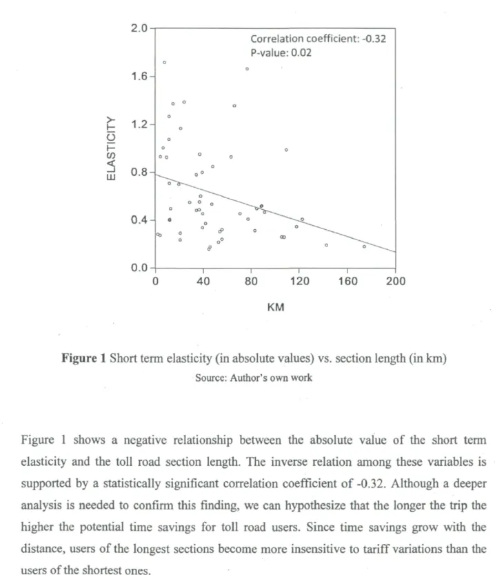
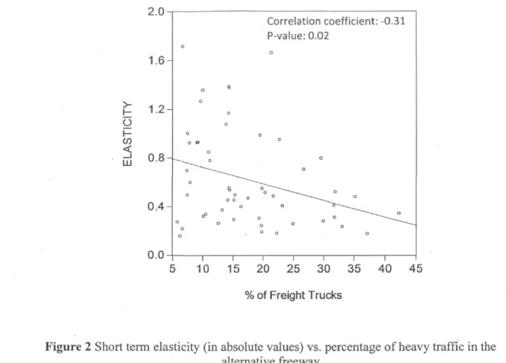
Figure 1 Short term elasticity (in absolute values) vs. section length (in km) 37 Figure 2 Short term elasticity (in absolute values) vs. percentage of heavy traffic in the

Introduction

This research is motivated by the need to provide policy makers with reliable tools allowing them to develop effective economic policies. Therefore, the objective of this study is twofold. First, we will estimate own-price demand elasticities for the largest Mexican tolled network. Second, we will determine which factors are more likely to explain the variation in our elasticity estimates.

The price elasticity of demand is one of the key parameters needed to design an appropriate tariff structure for tolled motorways (De Rus et al. 2000 and Rico Galindo 2005). Therefore, we expect that our results will help decision makers to improve those structures and also will let them evaluate potential traffic management strategies. Also by explaining why price demand elasticity values vary among road segments we will help to have a deeper understanding of what drives users' sensitivity to toll changes.

According to De Rus (2001), accurate price demand elasticity estimates are vital to promote an efficient use of road infrastructure. For instance, if in a situation of lower than expected demand for a specific toll road we found evidence that potential users are sensitive enough to tariff changes, then a toll reduction will increase traffic in this particular toll way and eventually income. This could be a desired outcome for policymakers especially if the toll-free alternative is saturated. However, if we are in the exact opposite case and traffic levels are higher than initially predicted, causing congestion or bottlenecks in the tolled motorway then tariff increases would reduce demand by diverting drivers to less used alternative routes. In both instances, an appropriate knowledge of toll elasticities would encourage better traffic management.

There are several examples that illustrate the consequences of lacking a precise knowledge of the information conveyed by price demand elasticity. Mexico's experience with its first road concessions program of 1989-1994 is probably one of the most striking cases (De Rus and Nombela 2000). As mentioned by Carpintero and Gômez-Ibanéz (2011) and Ruster (1997), the Mexican government established very high tariff maximums in exchange for short concession periods for the new toll roads constructed and operated by private firms. Most private concessioners decided to take advantage of this pricing leeway and charged the maximum toll allowed even though demand was probably very sensitive to high tariffs levels. Indeed, Mexico's Constitution required the presence of a parallel free road near to the tolled motorway. Hence, setting a high toll level has likely redirected a large volume of traffic to the free alternative (De Rus and Nombela 2000). This inadequate traffic structure was one of the main factors behind private motorway operators' bankruptcy and the subsequent financial rescue implemented by the Mexican government in 1997.

This public funded bailout had an initial cost of 1.8% of Mexico's Gross Domestic Product (GDP) reaching 2.2% of GDP in 2002 when a special government trust fund issued debt notes to help finance the tolled roads rescue and took over bank credits assumed originally by the former road concessionaires (CEFIP 2004). In light of this heavy burden over Mexico's public finances it becomes relevant to provide an instrument of economic policy to manage major public infrastructure. Therefore, there is a need for reliable price demand elasticity estimates of the country's main tolled motorway network. This would provide a framework under which it will be possible to analyze any proposed tariff structure change and its potential effect over a given network section.

Previous studies that have analyzed toll road demand have found that users of these road infrastructures are generally insensitive to price changes. However, tariff movements around certain critical values can considerably increase users' sensitivity to toll variations. Also some limited success has been observed when tolls have been used as traffic management tools. Furthermore, some evidence suggests that as toll levels increase

elasticity absolute values also increases. But perhaps the most important finding is that toll road users sensitivity to tariff changes mainly depends on traffic conditions in the alternative freeway.

We use a panel data regression methodology proposed by Matas and Raymond (2003) in order to obtain long and short term elasticity estimates for all the toll road segments in our sample. Since toll roads demand is not exclusively determined by tariff changes, we included in the regression other variables such as the fuel price and indicators of economic activity that are also likely to affect traffic volumes. Using this approach, we observe that in average Mexican toll road users are more sensitive to price changes than what is reported in other studies. However, this can be at least in part explained by Mexico's legal requirement that every toll road must have an alternative parallel free route nearby. We also find evidence of a negative relationship of the short term elasticity estimates (in absolute values) with the toll road section length and the percentage of heavy traffic in the parallel free road. This could mean that users of the longest toll segments are more insensitive to tariff variations because they benefit from higher time savings than users of the shortest road sections. Also, this might indicate that an increasing presence of freight trucks in the alternative freeway deteriorates its quality making toll road users' demand more inelastic.

This mémoire is structured as follows: Section 1 provides an overview of the history and current status of Mexico's toll roads network. Section 2 describes the main literature findings with respect to demand elasticity estimation for tolled highways. Section 3 defines the methodology necessary to develop the research objective and further clarifies the variables required to implement it. Section 4 mentions the information sources used during the empirical analysis. Section 5 summarizes the variables' main descriptive statistics. Section 6 introduces some econometric challenges and how they were overcome. Section 7 displays the elasticity estimates and presents some factors that explain their magnitude. This mémoire concludes with a presentation of our principal findings.

1. Background

Between 1989 and 1994 Mexico started an ambitious highways concessions program. Under this program almost three thousand kilometers of high specification roads were built.1 Notwithstanding the program's success on construction, road infrastructure projects

developed during this period suffered several shortcomings. For instance, building costs surpassed original estimations by a large margin. Operators' financial structures were put under great distress from the very beginning by these misleading forecasts. Furthermore, toll road demand estimations were too optimistic and new highways' actual traffic densities did not generate enough revenue to cover financial and operational costs. Compounding this situation was the decision by several private road operators to set their tariffs too high in a bid to recoup their investments faster. However, this strategy failed as traffic and income decreased thereby deepening concessionaries' insolvency. Several attempts by Mexican authorities and financial institutions to restructure the new highways debt burden proved insufficient. Mexico's economic crisis of 1995, also known as the "Tequila" crisis, skyrocketed domestic interest rates and completely shutdown foreign sources of financing. This pushed private road operators into bankruptcy and forced the Mexican government to instrument a rescue package for the whole toll road network. In 1997, the financial rescue was consolidated into a public trust fund known as the FARAC by its Spanish initials.

As a result of this intervention, the Mexican public sector now controls the largest toll road network in the country. According to Rico Galindo (2005) the federal government set up an expert panel with the task of developing a multi criteria tariff scheme for its toll roads. From the point of view of Mexican authorities the tolls proposed by the panel should be able to address the following three aspects of road infrastructure pricing: 1) long term

1 This section is based mainly on two studies: (1) Ruster, J. (1997). A Retrospective on the Mexican Toll Road

Program. Public Policy for the Private Sector. Note No. 125 September 1997, pp. 1-8. (2) Carpintero, S. and Gômez-Ibaflez, J.A. (2011). Mexico's Private Toll Road Program Reconsidered. Transport Policy. Vol. 18 No. 6, pp. 848-855.

2 Fideicomiso de Apoyo al Rescate de Autopistas Concesionadas (Support Trust Fund for the Rescue of

financial solvency, 2) recovery of maintenance and operational costs, and 3) traffic management.

The tariff panel includes representatives from different public entities such as the Treasury Ministry, the Transport and Communications Ministry and The National Public Works Bank (BANOBRAS), who manages the FARAC trust fund. Since the panel recommendations have not been made public it is hard to know exactly over which parameters it is basing its decisions. However, it is worth noting that the panel's methodological outline identifies income and price elasticities of demand as two of the key parameters needed to design an appropriate tariff structure for the FARAC network.

2. Literature Review

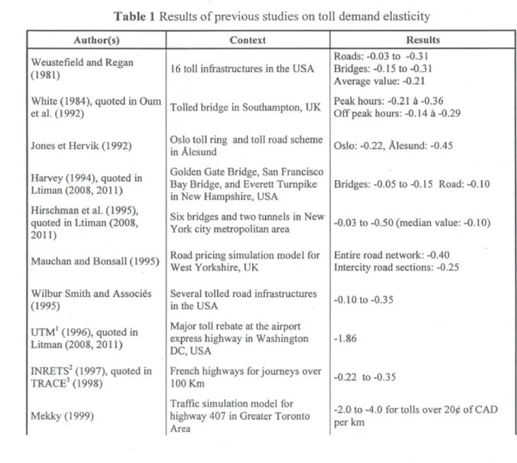
Table 1 summarizes the main results of the studies reviewed in this section and also shows empirical evidence reported by other authors with respect to price demand elasticity for tolled infrastructures. One of the main conclusions that emerges from this table is that, in most cases, the toll road demand is inelastic. However, the degree of inelasticity depends on several factors such as traffic conditions not only on the toll way but also on the alternative freeway.

Table 1 Results of previous studies on toll demand elasticity

Author(s) Context Results

Weustefield and Regan (1981)

White (1984), quoted in Oum etal. (1992) Jones etHervik( 1992) Harvey (1994), quoted in Ltiman (2008, 2011) Hirschmanetal. (1995), quoted in Ltiman (2008, 2011)

Mauchan and Bonsall (1995) Wilbur Smith and Associés (1995) UTM' (1996), quoted in Litman (2008, 2011) INRETS2 (1997), quoted in TRACE3 (1998) Mekky(1999)

16 toll infrastructures in the USA Tolled bridge in Southampton, UK Oslo toll ring and toll road scheme in Alesund

Golden Gate Bridge, San Francisco Bay Bridge, and Everett Turnpike in New Hampshire, USA

Six bridges and two tunnels in New York city metropolitan area Road pricing simulation model for West Yorkshire, UK

Several tolled road infrastructures in the USA

Major toll rebate at the airport express highway in Washington DC, USA

French highways for journeys over 100 Km

Traffic simulation model for highway 407 in Greater Toronto Area

Roads: -0.03 to -0.31 Bridges:-0.15 to-0.31 Average value: -0.21 Peak hours: -0.21 à-0.36 Off peak hours: -0.14 à -0.29 Oslo: -0.22, Âlesund: -0.45

Bridges:-0.05 to-0.15 Road:-0.10 -0.03 to -0.50 (median value: -0.10) Entire road network: -0.40

Intercity road sections: -0.25 -0.10 to-0.35

-1.86

-0.22 to-0.35

-2.0 to -4.0 for tolls over 200 of CAD per km

UTM (2000), quoted in Litman (2008, 2011) Matas and Raymond (2003) TCRP4 (2003)

TCRP (2003) and Burris et al. (2004)

Odeck and Brâthen (2008) Melandetal. (2010) Xing etal. (2010)

Holguin-Veras et al. (2011)

Representative sample of toll ways in the USA

Panel data for 72 Spanish toll road sections

SR 91 highway in Orange County, California (USA)

Variable road pricing scheme in Lee County, Florida (USA) 19 tolled infrastructures in Norway Toll ring removal in Trondheim, Norway

Interurban highway in Tomei, Japan

Six tunnels and bridges connecting New Jersey to New York City

Average value: -0.20 Short term: -0.21 to-0.83 Long term: -0.33 to-1.31 -0.40 to -0.90

Average value (1999): -0.14 Average value (2002): -0.08 Short term average value: -0.45 Long term average value: -0.82 Including time costs: -0.59 Excluding time costs: -0.22 -0.30 à -0.72

-0.11 à-0.24

1 UTM: Urban Transportation Monitor

2INRETS: Institut national de recherche sur les transports et leur sécurité Optional Institute for Research on

Transport and Transport Safety)

3 TRACE was an European research project on private travel road costs and their effects on transport demand 4 Transit Cooperative Research Program

Source: Author's review of various studies with additional information from Table 1 of Matas and Raymond (2003) and Table 1 of Odeck and Brâthen (2008).

Matas and Raymond (2003) estimate a demand equation using a panel data sample of Spanish toll roads over the 1980-1998 period. The level of traffic is assumed to depend upon toll variations but also on other factors as economic activity growth, changes in fuel price and regional characteristics such as the affluence of tourists. The authors find short run elasticities varying from -0.21 to -0.83 and long run estimates between -0.33 to -1.31. They also notice that demand is more price-sensitive in toll roads that compete with freeways that experience low congestion levels, since drivers probably considérer those alternatives as a good substitute to the toll way.

The Transit Cooperative Research Program (TCRP) shows similar results as Matas and Raymond's study, particularly for the Riverside Freeway (SR 91) in Orange County, California. The TCRP report on a series of studies commissioned by the California Department of Transportation intended to analyze traffic patterns between tolled express lanes built in the middle of SR 91 and their parallel toll-free alternatives. Two methodological approaches were used to estimate price demand elasticities for the SR 91 corridor. First, elasticities were calculated by comparing traffic volume before and after the express lanes' first toll increase in January 1997. This initial analysis finds a toll elasticity of -0.4 in the eastbound lane and of -0.5 in the westbound one. Afterwards, a second approach, using surveys results and transport network data to calibrate discrete choice models for travel demand, finds that drivers were more sensitive to tariff changes with price elasticities between -0.7 to -0.9. This result is likely due to the existence of an adjacent freeway option with acceptable service conditions (TCRP 2003).

According to a review by Litman (2008, 2011), the freeway conditions seem more relevant inside urban contexts where the users of the toll-free alternatives usually face high congestion levels. Hirschman et al. (1995) find that given the high level of congestion in the free alternatives, the demand for toll bridges and tunnels in the New York metropolitan area is highly inelastic, with a median value of-0.10.3 Harvey (1994) finds similar results

for. the San Francisco metropolitan area's bridges and for a tolled motorway in New Hampshire, with elasticity estimates ranging from -0.05 to -0.15.

Other studies reviewed by Litman (2008, 2011) seem to indicate that the previous findings of inelastic toll road demand hold for different contexts inside the United States. For instance, a study performed by the New Jersey Turnpike Authority finds an elasticity of -0.2 for small toll increases within a representative sample of toll ways in the U.S. (UTM 2000). Nevertheless, in some circumstances a much higher level of sensitivity to tariff has

3 Matas and Raymond (2003) report that if we only considered the significant coefficients in the equation

been observed. When the Dulles Greenway toll road, an express highway heading to Washington D.C. airport, reduced its tariff by 43% (from $1.75 to $1.00) the daily demand grew by 80%, indicating an elasticity demand close to -2 (UTM 1996).

Some studies results suggest that there exist a critical point above which the demand reacts more than proportionally to toll changes. For example, Mekky (1999) analyzes traffic patterns for highway 407 in the Greater Toronto Area (GTA), a tolled option to the highly congested 401 highway. The author uses a sequential four-stage model4 with different

tariffs to replicate and forecast daily trips on highway 407. Mekky finds price elasticities in a range of -2.0 to -4.0 for tolls over 200 of Canadian dollar (CAD) per km, which led him to conclude that the absolute value of the elasticity increase with the toll level. He also shows evidence that a tariff higher than 100 of CAD per km would produce a significant reduction in traffic volumes and toll revenues.

The presence of this critical toll level seems to point to a trade-off between the travel time savings and the pecuniary cost of using the toll road. Toll reductions around this turning point would transform the potential gain in travel time attractive enough to cause a significant transfer from freeway's users to the toll way. Similarly, if there is a tariff increase near this critical toll level it is possible that a considerable number of drivers will choose the free alternative (TCRP 2003). This would be reflected in price elasticities higher than the ones usually found in the specialized literature.

Several studies have also focused on how different price mechanisms affect toll road traffic during the day making a distinction between peak and off-peak hours. In 2001, the Port Authority of New York and New Jersey implemented the use of intelligent cards on its system of toll tunnels and bridges giving a discount to users during off-peaks hours. According to evidence found by the Federal Highway Administration (2001) there were

10 some small traffic increases (around 7%) in the traffic during the off peak periods, particularly during the hours just before the period of maximum demand during the mornings. They also found small decrease in the utilization of the toll infrastructures during the maximum peak hours in the morning (-7%) and the afternoon (-4%). In 2000 the New Jersey Turnpike Authority applied a 20% increase in peak-period tariff exclusively. In this case, the increase in traffic was lower during peak hours compared to the increase in total demand. Moreover, there was a slight decrease in the proportion of users during the maximum demand period, particularly during the afternoon (Federal Highway Administration 2001).

The TCRP (2003) describes another tariff reduction scheme applied during off-peak hours at the two toll bridges of Lee County, Florida in 1998. The discount was only offered to drivers using electronic toll collection devices, which represented around 25% of the bridges' traffic. These users obtained a 50% toll discount during off-peak periods. The aggregate traffic pattern on the bridges didn't significantly change after the implementation of the toll reduction program. However, demand shifts were observed among drivers eligible for the discount. Those users started to travel more often during the off-peak periods, with the main trips increase occurring just before the morning rush hour. One of the bridges showed an 18% increase from 6:30 to 7:00 AM which implied a toll elasticity of-0.36. While on the second bridge traffic grew by 10% during the same period leading to a price elasticity of-0.20.

The TCRP report on the Lee County bridges' variable pricing scheme includes price demand elasticity estimates for all off-peak periods. These were calculated by comparing demand levels during the pre-discount period of January to July 1998 and the post-discount period of January to July 1999. These toll elasticities vary from a minimum of-0.03 in the post-PM5 peak hour to a maximum of-0.36 during the pre-AM peak period6 (TCRP 2003).

11

Burris et al. (2004) continued to analyze the variable toll scheme in Lee County from 1999 to 2002. These authors find a significant reduction in the elasticity compared to those originally reported by the TCRP. For instance, for one of the bridges, the maximum elasticity value decline from -0.36 in 1999 to -0.18 in 2002. In order to further compare both studies, we calculate the mean price elasticity for both bridges using the TCRP 1999 data and find a value of -0.14, while if we compute the same average with Burris et al. 2002 data we obtain a result of only -0.08.

Burris et al. (2004) conclude that this reduction in the absolute values of the bridges' elasticities could be explained by two factors. First, during the observed period the nominal amount of the discount remained stable at approximately 250 of US$ per trip. Therefore, it is conceivable that some users started to regard this potential monetary saving as too small to merit a modification in their travel behavior. This would be reflected in fewer drivers shifting to the off-peak periods and since the percentage of toll rebate stayed constant at 50% this would give us smaller elasticity estimates. Second, a telephone survey conducted in July 2001 showed that only 18% of the eligible discount users had the option of flexible working hours. Hence, near 2002 a high proportion of the variable pricing scheme potential beneficiaries were faced with significant schedule constraints. This probably made them highly insensitive to the tariff discount offered in off-rush hours.

More recent studies by Odeck and Brâthen (2008) and Meland et al. (2010) analyze the impact of tolls in Norway. The former authors study 19 road infrastructures where tolls were implemented or removed during a 15 years span (from 1987 to 2002). They use a combination of arc elasticity techniques and time series regressions to estimate an average

6 From 6:30 to 7:00 AM.

7 The elasticity for 1999 represents the discount period from 6:30 to 7:00 AM while the value for 2002 stands

for the pre-PM peak hour promotion (from 2:00 to 4:00 PM).

8 Since Burris et al. (2004) affirm that the toll discount didn't have an impact on traffic growth during the 6:30

12 short term elasticity of-0.56 and a mean long term elasticity of-0.82. They also established that elasticities vary with roads characteristics and that it seems to exist a positive relationship (although a weak one) between the elasticity and toll levels.10

Meanwhile, Meland et al. (2010) analyze the removal of the Trondheim toll cordon on December 31, 2005. Norwegian toll cordons or rings are road pricing schemes that charge users when they enter a particular city area (including, but not limited to, the downtown). Their main purpose is to finance road investment and public transportation. Although, Trondheim scheme had also a variable pricing component used for traffic management purposes.

According to Meland et al. (2010), all toll projects in Norway are approved for a maximum period of 15 years. Therefore, once the Trondheim toll cordon reached the 15 year mark, local authorities felt compelled to remove it, even when it was widely considered a financial and traffic management success. The authors compare demand levels before and after the toll ring closure, they found a peak-hours average traffic increase of 11.3%, with a higher afternoon surge of 15.5%. Based on these results they calculate the change in the average generalized cost per car trip in Trondheim one year after the toll ring was removed. The authors work with two scenarios depending on whether drivers take the increase in time costs (due to congestion growth in Trondheim former cordoned areas) into account or not. Excluding the travel time rise, they obtain a 30% reduction in generalized costs and an implicit elasticity of -0.22. However, if motorists in Trondheim take into account the increment in time costs then the estimated decrease in generalized costs is of only 12.4%." Under these circumstances, the authors find a price elasticity of-0.59.

9 They analyzed three types of tolled infrastructures: rural roads, trunk roads and urban motorways. 10 Implying that as toll levels increase elasticity values also increases.

1 ' Because the increase in time costs partially offsets the toll cordon elimination effect over the generalized

13 More recent studies, such as Xing et al. (2010) and Holguin-Veras et al. (2011), have been more focused on how to switch traffic between off peak and peak periods using different tariff structures. Holguin-Veras et al. (2011) estimate elasticities between -0.11 to -0.24 for several toll infrastructures connecting New Jersey to New York. They also found that drivers faced with a higher toll during peak hours are more likely to shift mode (carpooling or using public transport) rather than travelling during off peak periods. These authors conclude that this response is probably due to scheduling constraints (i.e. be on time at work, etc) preventing car users to fully take advantage of the differentiated toll structure.

Xing et al. (2010) studied different traffic management strategies implemented on the Tomei Expressway in Japan. These measures consisted in offering tariff discounts during major Japanese holidays as well as during off-peaks periods, but only for vehicles equipped with electronic toll collection systems. The authors calculate the demand shift from rush hours to off-rush hours and then estimate arc elasticities that vary from -0.30 to -0.72. The variation on these elasticities seems to depend on the specific holiday and the time period where toll discounts were offered. In general the authors find that drivers were more sensitive to discounts during off peak morning hours and when toll savings exceeded the 1,000 yens threshold. Based on these results, the authors calibrate a traffic flow model and conclude that without the toll discount program delay times and congestion levels during peak hours would have been higher to the observed ones.

In summary, the main conclusions that can be drawn from the literature are the following. First, several studies find low levels of price demand elasticities, which imply that toll road users are not very sensitive to tariff variations. However, toll elasticity also appears to depend upon the traffic conditions on the alternative freeway. In particular, drivers would be more sensitive to tariff changes if the toll-free option had a good service level (low road congestion, acceptable levels of freight traffic, etc). Also, when studies distinguish between the short and the long term they find higher absolute values of price elasticity in the long run. This could be because in the long run toll road users are able to better adjust their

14 travel pattern in response to tariff variations. Furthermore, there is evidence that not only price changes affect tolled motorways demand but there are also other factors such as economic conditions and fuel costs that may also have an impact on it.

In addition, some authors find a critical toll level above which demand sensitivity becomes much higher. Hence, tariff adjustments near this critical point would be reflected in steep changes in the demand and in elasticity estimates near or higher than one (in absolute values). Moreover, at least some evidence suggests a positive relationship between the toll level and the absolute value of the price demand elasticity. Finally, several studies indicate that switching traffic between peak and off peak hours using variable toll schemes is possible. However, the presence of daily schedule constraints probably hinders the effectiveness of these traffic management programs.

From the previous review we can conclude that most of these studies obtain toll demand elasticities by comparing situations with and without tariff. This means that they perform elasticity estimates when a particular tariff structure is implemented or removed and comparing traffic behavior during brief transition periods. Only a few published articles, such as Matas and Raymond (2003), have introduced methodologies to study the impact of toll changes in road transport systems using panel data.

In view of the above, the research developed in this study will contribute to enrich our understanding of price demand elasticity estimation in a context of large tolled networks where panel data regressions can be applied. Also there is an additional benefit given that it studies a developing country (Mexico), an area where there is still a gap in the relevant literature.

15

3. Methodology

This section starts by defining the concept of elasticity. According to Varian (1990) price demand elasticity can be defined as the percent change in quantity divided by the percent change in price. Therefore, the elasticity concept provides a measure of how responsive demand is to a particular price change in a unit-free fashion since everything is expressed in percentage terms. For discrete price changes, price demand elasticity (£PD) can be defined

as follows:

Thus, any elasticity could be calculated as the ratio of price to quantity multiplied by the demand function slope (Varian 1990). For the continuous case, which implies infinitely small price variations, it is possible to use derivatives to reformulate the elasticity definition:

(2) £PD ~

dQ P_

16 Finally, for the special case of a logarithmic demand function, which implies a constant elasticity along the demand curve, expression (2) can be written as:l2

dlnQ

(3) £pn = ~

If we are dealing with a normal good (i.e. if its consumption increases as income raises, holding price constant) and if the law of demand holds13 we should expect a negative sign

for the price demand elasticity (Varian 1990).

Continuing with Varian (1990), it is possible to classify any good or service demand according to its elasticity's magnitude. For instance, if demand elasticity is greater than 1 in absolute value then the demand for such good is called "elastic", which implies that it is very sensitive to price changes. A demand that is generally unresponsive to price variations is called "inelastic" and is associated with an elasticity value of less than 1 in absolute terms. Finally, if \sPD\ is exactly equal to 1 then demand elasticity is "unitary" which implies

a proportional relation between price and quantity.

Therefore in our context price demand elasticity estimates would reflect how sensitive traffic on tolled motorways is to tariff changes. If users regard these road infrastructures as normal goods then we should expect to obtain a negative sign in our elasticity calculations. As illustrated in the literature review, we expect the toll elasticity to depend upon different factors such as the traffic conditions on the alternative freeway.

12 Varian (1990) and other classic microeconomics manuals offer a very straightforward proof of the

equivalence between all elasticity formulas presented in this section.

13 According to Jehle and Reny (2000), the law of demand states that any decrease (increase) in the own price

17

Regarding the empirical strategy, this research will follow the methodology developed by Anna Matas and Josep Luis Raymond for Spanish motorways.14 We will use panel data

regression techniques in order to obtain the toll elasticity on the different road segments of the FARAC network. Specifically, we combine information on the level of traffic and toll by road segments for the years 1999 to 2010. By combining two sources of variability (time and segment), panel data allows the estimation of richer models. Also note that the different road segments belong to 18 different highways.

Based on the models proposed by Matas and Raymond (2003) and Odeck and Brâthen (2008), our toll road demand equation should have the following overall structure:

(4) AADT =f(EA,FP,T,VOCT,TCT,VOCF,TCF,0,D)

Hence, we expect the level of traffic on a road segment - measured by the Annual Average Daily Traffic (AADT) - to depend upon indicators of the general level of economic activity (EA), the level of fuel price (FP), the toll on the road section (7), the level of vehicle operating costs (other than fuel costs) both on the toll road (VOC ) and on the free alternative (VOCf), the time costs on the tolled segment (TCT) and the freeway (TCf). The

level of demand on a road section will also depend on particular characteristics of the origin and destination. Thus, in expression (4) O and D represent trip generation and attraction factors which influence the volume of traffic on a given toll road.

14 Matas, A. and Raymond, J.L. (2003). Demand Elasticity on Tolled Motorways. Journal of Transportation

18 Unfortunately, we do not have data on VOCT, VOCF, TCT, TCF and on the O and D

factors.15 However, following Matas and Raymond (2003), it is reasonable to assume that

the operating cost and travel time have remained relatively constant over time. This assumption is justified by the fact that the road network didn't experience major changes (such as the construction of an additional traffic lane) during the period covered by our data. Moreover, the Transport and Communications Ministry probably kept a standard policy of road maintenance for both the toll roads and the freeways. Therefore, it is unlikely that during the years of public management the toll ways gained any additional competitive advantages (in terms of lesser VOC or improving time savings) over the toll free alternatives. Moreover, it is highly unlikely that network congestion issues have favored the tolled motorways over the freeways (or vice versa) since both deal mainly with intercity and regional traffic where congestion is hardly a problem.

Also, significant changes in trip generation and attraction factors (O and D) usually only occur in response to major economic and/or social shifts. The last time this happened in Mexico was during the late 80's and early 90's when the government opened the economy to foreign trade and investment. This event is not likely to have significantly altered the O and D factors of the tolled motorways included in our analysis since all of them began operating at the end of Mexico's economic liberalization process (see Table 2 in the next section). Also, the Mexican National Population Council (CONAPO) states that during the last census period (2001 to 2010) Mexico's population growth remained stable with no sudden breaks from previous observed trends. Therefore, it is reasonable to assume that the O and D factors have been relatively constant over the 1999 to 2010 period.

15 We would require an extensive fieldwork in order to obtain VOC and time savings information for every

cross-section in our sample. Also, we would need an origin-destination survey covering the entire road network to identify the main poles of trip generation and attraction.

16 The major population trends are: an increase in urban population, a diminishing fertility rate and a higher

19 Hence, these different O and D factors together with the VOC and time costs can be captured by including road segment fixed effects in our demand equation. More specifically, we can estimate the following model:

(5) AADT, = a, + /llhEAhl+/32FP, +J3ilTll + SUM„ + »u

Where the subscript / denotes each toll road segment, r is an index representing the period (years in our case), and the subscript h represents every highway in our sample (eighteen).17

In expression (5) variables AADT and T vary within time and between toll road sections, EA changes with time and across highways, and FP only changes along with time while the fixed effects vector (a.) varies exclusively across road segments. Finally, u represents the error term of the regression model.

From the variables previously introduced, we only added in equation (5) the dummy variable M with the purpose to capture any major change in the relevant road network. For example, the opening of a new complementary or alternative road, with or without toll, near a tolled section would be incorporated into the model with a dummy variable that will take a value of one from the beginning of operations of this new route. These dummy variables would help us to maintain our assumption that the fixed effects vector reflects factors that remain constant over time since any major change would be capture by M.

As we can see from equation (5), the fuel price coefficient (/?_>) will give us a unique estimate for all sections i. The reason behind this assumption is because fuel prices in Mexico only vary with respect to t and not among cities18 or regional markets. As a matter

of fact, any fuel price in Mexico is uniformly determined throughout the country by the

17 A highway has several different toll sections.

20

federal government. Thus, it is reasonable to assume that this variable behavior will equally impact all road segments in our tolled network.

Since, as noted by Matas and Raymond (2003) and Odeck and Brâthen (2008), demand for toll roads is expected to increase with income we include in (5) the variable EA in order to capture this income effect. However, it would be difficult to assign individual economic indicators to each section i in the model. Nevertheless, it is possible to link regional variables with the highways where each road segment belongs. Therefore, the coefficient Pih would have the same value for all toll road sections / inside the same highway h, but it

would differ across highways.

We also expect that this approach would allow us to reflect Mexico's regional economic disparities in our demand equation. We can use two readily available regional economic indicators to approximate the impact of variable EA on toll roads demand. The first one is GDP per capita defined as real regional gross domestic product divided by the population in the relevant area while the second one is wage income. This indicator is defined as the real average weekly earnings times the number of salaried workers in a given region. Which indicator is used in a particular highway is decided by how well each indicator helps us to explain toll road demand in its own region.19

The demand equation presented in (5) is a static model which means that all variation in the dependent variable is explained by the current value of the explanatory variables. The price demand elasticities obtained from this kind of models are usually placed between the short and long run elasticity estimates provided by a dynamic model. Therefore, in order to clearly differentiate between short and long term price effects we need to introduce a dynamic structure in our static demand equation. Following Matas and Raymond (2003)

19 The descriptive statistics of these indicators and of the rest of the variables used in our analysis are

21

and and Odeck and Brâthen (2008), we decided to transform our static model into a dynamic one by introducing as an explanatory variable the lagged value of the dependent variable AADT. Therefore, we can rewrite expression (5) as follows:

(5a) AADT,, = al+/6ihEAhl +/32FPt +/33,Tll + y,AADTII_l +SuMlt +ult

The intuition behind the dynamic structure introduced in (5 a) is that toll road users do not react immediately to changes in the explanatory variables but that they adjust their travel patterns with a delay and over several periods. Therefore, past values of the AADT in a given segment / contain relevant information that would help us to explain the current level of the dependent variable (Matas and Raymond 2003).

In order to derive long term elasticities from expression (5a) we only need to divide coefficient /??. by 1 - yi- m general, 1 - yi represents an adjustment factor which measures

how quickly toll road users adapt to changes in the explanatory variables. Thus, the larger the value of coefficient yt the lower the adjustment speed and the greater the discrepancy between the short and long run elasticities (Odeck and Brâthen 2008).

In summary, expression (5a) includes all the relevant information for our analysis. Specially, this demand equation will allow us to calculate long and short term price demand elasticities for each road segment / in our sample, which is the main objective of this research.

22

4. Data Base

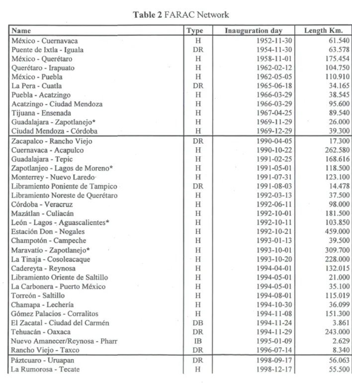
Table 2 shows FARAC network structure at the end of 2007. The information in Table 1 is divided in three sections according to the operations start date of each toll way inside FARAC.

Table 2 FARAC Network

Name Type Inauguration day Length Km.

Mexico - Cuernavaca H 1952-11-30 61.540

Puente de Ixtla - Iguala DR 1954-11-30 63.578

Mexico - Querétaro H 1958-11-01 175.454

Querétaro - Irapuato H 1962-02-12 104.750

Mexico - Puebla H 1962-05-05 110.910

La Pera - Cuatla DR 1965-06-18 34.165

Puebla - Acatzingo H 1966-03-29 38.545

Acatzingo - Ciudad Mendoza H 1966-03-29 95.600

Tijuana - Ensenada H 1967-04-25 89.540

Guadalajara - Zapotlanejo* H 1969-11-29 26.000

Ciudad Mendoza - Cordoba H 1969-12-29 39.300

Zacapalco - Rancho Viejo DR 1990-04-05 17.300

Cuernavaca - Acapulco H 1990-10-22 262.580

Guadalajara - Tepic H 1991-02-25 168.616

Zapotlanjeo - Lagos de Moreno* H 1991-05-01 118.500

Monterrey - Nuevo Laredo H 1991-07-31 123.100

Libramiento Poniente de Tampico DR 1991-08-03 14.478

Libramiento Noreste de Querétaro H 1992-03-13 37.500

Côrdoba - Veracruz H 1992-06-11 98.000

Mazâtlan - Culiacân H 1992-10-01 181.500

Leôn - Lagos - Aguascalientes* H 1992-10-11 103.850

Estaciôn Don - Nogales H 1992-10-21 459.000

Champotôn - Campeche H 1993-01-13 39.500

Maravatio - Zapotlanejo* H 1993-10-01 309.700

La Tinaja - Cosoleacaque H 1993-10-20 228.000

Cadereyta - Reynosa H 1994-04-01 132.015

Libramiento Oriente de Saltillo H 1994-05-01 21.000

La Carbonera - Puerto Mexico H 1994-05-01 35.100

Torreôn - Saltillo H 1994-08-01 115.019

Chamapa - Lecheria H 1994-10-30 36.099

Gômez Palacios - Corralitos H 1994-11-08 151.300

El Zacatal - Ciudad del Carmen DB 1994-11-24 3.861

Tehuacân - Oaxaca DR 1994-11-29 243.000

Nuevo Amanecer/Reynosa - Pharr IB 1995-01-09 2.629

Rancho Viejo - Taxco DR 1996-07-14 8.340

Pâztcuaro - Uruapan DR 1998-09-17 56.063

23

Reynosa - Matamoros H 1999-04-30 44.000

Ignacio Zaragoza IB 1999-04-30 0.810

Uruapan - Nueva Italia DR 2000-06-21 59.437

Aguadulce - Cârdenas H 2000-11-09 53.300

Tihuatlân - Gutierrez Zamora H 2001-09-22 37.297

Nueva Italia - Lazâro Cârdenas DR 2001-10-17 155.000

Las Choapas - Ocozocoautla DR 2002-09-06 198.000

Ent. Aeropuerto los Cabos - San José del Cabo DR 2002-10-17 20.200

Salina Cruz - Tehuantepec - La Ventosa DR 2003-05-15 75.500

Total Length Km. 4504.476

H = Highway (two traffic lanes in each direction). DB = Domestic Bridge.

DR = Direct Road (one traffic lane in each direction) IB= International Bridge.

* On October 3, 2007 these motorways were divested from the FARAC network and concessioned to the firm Red de Carreteras de Occidente, S. de R L. de C. V.

Source: 2007 CAPUFE Statistical Yearbook.

The first section includes the oldest road infrastructure. These sections originally belonged to a network operated directly by the Mexican Transport and Communications Ministry or were part of previous state sponsored road trust funds that were later consolidated into FARAC. The second section includes toll ways directly involved in the 1997's public financial rescue of Mexican concessioned highways, which itself gave birth to FARAC. The last section of Table 2 corresponds to road infrastructure projects funded with resources channeled through FARAC and inaugurated after the public bailout of private road investors.

Our data set focusses on the second section of Table 2 namely the toll ways originally involved in the 1997's financial rescue of the Mexican concessioned road network. Specifically, we will only include the 18 FARAC highways with two traffic lanes in each direction. We therefore exclude from our analysis special purpose infrastructures such as international bridges and direct roads which only have one traffic lane in each direction.

These 18 highways constitute a relatively homogeneous sample since they have the same number of lanes in each direction and they have been in operation for several years thereby

24

providing a good time series. Finally, Mexican authorities' dilemma about which tariff policy would be better suited for the FARAC network originally concerns those 18 toll ways that were financially rescued from private concessionaires. The older roads, included in the first segment of Table 1, probably already had a defined tariff structure when they were incorporated inside the FARAC.

Also, there are several reasons to believe that those 18 tolled motorways probably have a tariff structure that can be considered as "exogenous". First, as we mentioned in the background section, at least three government entities (BANOBRAS, the Finance Ministry and the Transports and Communications Ministry) participate in the expert panel in charge of determining FARAC network's tariff structure. It is therefore likely that tolls are the result of a consensus reaching process and are based on several factors besides cost recovery. Second, there is evidence that the government allows for political considerations to influence its toll policy. For instance, at the end of 2007 Mexican President Felipe Calderôn announced a combination of tariff freezes and reductions for the whole FARAC network as a series of steps designed to "help Mexican families' economy" (Secretaria de Comunicaciones y Transportes 2007). These special measures were in place for all 2008 and most of 2009, and they were not completely reversed. Third, even when some FARAC s motorways were auctioned again in 2007 and 2009 to private operators, the Ministry of Transports and Communications imposed strict toll structures (Red de Carreteras de Occidente 2010). Hence, it is likely that CAPUFE20 or any private firm who

took over segments of the FARAC network have taken tariffs as given.

The main data source is the statistical yearbooks of CAPUFE. These documents display information on traffic and tariffs for the FARAC network from 1999 until 2010. The CAPUFE yearbooks do not only contain general data about the toll roads but they also

20 It is the acronym in Spanish for Caminos y Puentes Fédérales de Ingresos y Servicios Conexos (Federal

Toll Roads and Bridges, and Related Services). CAPUFE is a special decentralized organism created by the Mexican Ministry of Transport and Communications to operate public road infrastructure.

25 include specific information regarding each road segment. Table 3 is an example of how the information is presented for the Monterrey-Nuevo Laredo highway in 2007.

Table 3 Monterrey - Nuevo Laredo Highway (2007)

Section Vehicle AADT Tariff1 Length Km Tariff/ Km

Monterrey - La Gloria (D) 5,832 192 123 1.56

Monterrey - Sabinas (11 )

Sabinas - La Gloria (12) Automobile2

28 60 109 83 77 46 1.41 1.81 Monterrey - Agualeguas (I) 468 78 57 1.37

12007 Mexican pesos, official toll at 16/01/07.

2 This vehicle category includes cars, motorcycles, and pickup trucks.

D (Direct): Users that drive the entire motorway.

I (Intermediate): Users that drive only one section of the toll road.

Source: Author's own work based on CAPUFE information.

Table 3 describes two different kinds of users for the Monterrey-Nuevo Laredo highway: Direct users, who drive the complete toll road length; and Intermediate users, who only drive one section of the toll way. The direct users are described in the section Monterrey-La Gloria (named as the village where the last toll booth is located), while the intermediate users are divided in three different categories depending on the section they use. In all cases, the AADT and the associated tariff for each category is shown accordingly with the traveled road section.

The other explanatory variables needed, such as economic activity indicators and fuel prices, are available through the Labor and Energy Ministries, the National Institute of Statistics and Geography (INEGI) and Mexico's Central Bank (BANXICO).

26

5. Data description

We have information for 133 road segments from 1999 to 2010. In order to choose which road sections to include in our final analysis, two selection criteria were used. First, we only considered segments with complete traffic and toll data for the entire 12 year-period. Second, it was decided to exclude sections that could be affected by the opening of new motorway stretches and/or by the installation or removal of toll booths. Mainly because that kind of network modifications probably changed the way traffic patterns were recorded by CAPUFE in its yearbooks. Based on the above criteria, 91 toll sections were finally selected for a period of twelve years. This provided us with

1092 observations to develop the data panel regression explained in the previous section.

For these 91 road sections we calculated the AADT of those vehicles classified as type "A"21 by CAPUFE. We also obtained the total length in km and the annual average toll22

for each segment. Using the previous information we determined the toll per km so we can have a price variable without the distance effect. Normalizing the tariff by the distance give us a better sense of the real price faced by toll road users23 and is a common practice in the

relevant literature (Matas and Raymond 2003).

For the fuel price variable we used the annual average price per liter of the gasolines sold in Mexico. As we discussed before, we used GDP per capita and wage income in order to

21 Vehicles type "A" includes cars, motorcycles and pickup trucks.

22 In all road segments considered we found different tolls for the same year. Therefore, we calculated a

weighted annual average tariff based in the number of days that each toll was in effect during a given year.

23 For instance, imagine two roads, one with a length of 30 km and the other one with just 10 km. Now, let's

assume that both charge $30 dollars per vehicle. Both roads seem to cost the same, but actually the users of the second road are paying three times more per km than the users of the first road.

24 We weighted the annual average price of the two type of gasolines sold in Mexico by their share in the total

sales volume of gasoline reported by the Mexican state oil company (PEMEX). An additional adjustment was made to take into account the proportion of gasoline sold in border towns. Gasoline sales in this part of the country have a lower value added tax than gasoline sold elsewhere. Hence, the border towns enjoyed a lower final gasoline sale price than the rest of Mexico,

27

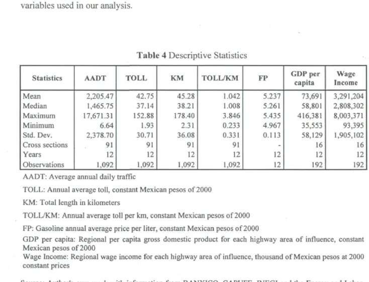
capture the effect of economic activity over toll roads demand. All the price variables and the GDP per capita are expressed in constant Mexican pesos of 2000. The fuel price and the toll per km were deflated using the consumer price index published by BANXICO while the GDP per capita was transformed in real terms through the GDP's implicit price deflator calculated by INEGI. The following table presents the main descriptive statistics of the variables used in our analysis.

Table 4 Descriptive Statistics

Statistics AADT TOLL KM TOLL/KM FP GDP per _{capita Income} Wage

Mean 2,205.47 42.75 45.28 1.042 5.237 73,691 3,291,204 Median 1,465.75 37.14 38.21 1.008 5.261 58,801 2,808,302 Maximum 17,671.31 152.88 178.40 3.846 5.435 416,381 8,003,371 Minimum 6.64 1.93 2.31 0.233 4.967 35,553 93,395 Std. Dev. 2,378.70 30.71 36.08 0.331 0.113 58,129 1,905,102 Cross sections 91 91 91 91 - 16 16 Years 12 12 12 12 12 12 12 Observations 1,092 1,092 1,092 1,092 12 192 192

AADT: Average annual daily traffic

TOLL: Annual average toll, constant Mexican pesos of 2000 KM: Total length in kilometers

TOLL/KM: Annual average toll per km, constant Mexican pesos of 2000 FP: Gasoline annual average price per liter, constant Mexican pesos of 2000

GDP per capita: Regional per capita gross domestic product for each highway area of influence, constant Mexican pesos of 2000

Wage Income: Regional wage income for each highway area of influence, thousand of Mexican pesos at 2000 constant prices

Source: Author's own work with information from BANXICO, CAPUFE, INEGI and the Energy and Labor Ministries.

As we can see in Table 4, there is a wide variation in the values of the AADT and the average toll per km. This wide range of tariffs and traffic volumes will allow us to estimate price elasticities that reflect very different demand conditions in each road segment. The fuel price shows much less variability than the previous variables. This is

28 probably because the Mexican federal government controls the gasoline price and its determination is more linked to political and fiscal concerns than to actual market forces. The wide scope of values for the GDP per capita and the wage income is likely to reflect Mexico's large regional disparities. Finally, we group the data for these latter variables in 16 highways instead of 18 because two of our highways are so close to neighborly motorways that we treat them as belonging to the same influence area as their neighbor highways.

29

6. Some econometric issues

Before we can estimate the model presented in the methodology section we should discuss some econometric issues. When we introduced expression (5a) we added a lagged dependent variable in order to introduce dynamic effects in our demand equation. However, as mentioned by Bilotkach and Huschelrath (2010), Crotte (2008) and Murray (2006), this is likely to cause an endogeneity problem in our model since the lagged variable is going to be correlated with the regression's error term.

The lagged dependent regressor will be correlated by construction with the individual effect ott (fixed or random) and with lagged value of the error term. Furthermore, the lagged term could also be correlated with current values of the error term if this is serially correlated (Arellano 2009). Therefore, due to the presence of endogeneity in the lagged regressor we will obtain biased and inconsistent estimators if we estimate our demand equation using a classic OLS specification (Murray 2006).

The traditional approach of instrumental variable (IV) estimation using additional lags of the dependent variable cannot overcome the endogeneity problem because any lagged instrument will also be correlated with its corresponding error term. However, an alternative version of the IV estimator can be used if the variables are transformed using first-differences (FD). Indeed, a FD estimation which employs the correct lags of the dependent variable will produce consistent parameter estimates (Cameron and Trivedi 2009).

Although the FD estimation removes the individual effect a., the lagged dependent variable Ay_,t-i is still correlated with the error term L\eit. Because the lagged element y^-i within

30

ei,t-i (Roodman 2006). Therefore, in order to solve our endogeneity problem we need to

find an instrument for Ayj t_x that is not correlated with Ae; t.

For the FD estimator, Anderson and Hsiao (1981)25 suggested using Ay£ t_2 = y.,t-2 —

yix-3 and y^t-2 as instruments for the lagged dependent variable since both are related to Ay.,t-i through y_/t-2 and uncorrected with t\ei t. However, Arellano (1989), Arellano and

Bond (1991) and Kiviet (1995)26 show that the lagged level term yii t-2 performs better as

an IV than the lagged difference instrument Ay; t_2 since using the latter results in

estimators with very large variance.

To improve the efficiency of the IV estimator we can use additional lags of the dependent variable as instruments. For instance, with seven periods (t = 1) and instrumenting for Ay.,t-iwith only lagged level terms at / = 3 there is one available instrument ( y ^ ) that is not correlated with à ei 3. However, at t = 4 there are two potential IV, yt l and yi 2,

uncorrected with Ae£ 4. Following with this progression, at / = 5 we have three available

instruments (y_.i,yi,2 and y ^ ) , at t = 6 we can add yi A to our previous count to reach a

total of four IV, and finally at / = 7 there are five potential instruments, y iv ...,y..s. If we

add up all the previous available instruments for each period we find 15 potential IV for the lagged dependent variable Ayf t_x (Cameron and Trivedi 2009).

This kind of IV estimator that uses further lags of the dependent variable as additional instruments is known as the Arellano and Bond (AB) estimator after Arellano and Bond's 1991 seminal article where the authors proposed and detailed its implementation. As the

25 Cited by Judson, R. and Owen, A. (1997). Estimating Dynamic Panel Data Models: A Practical Guide for

Macroeconomists. Finances and Economics Discussion Series. No. 1997-3. Board of Governors of the Federal Reserve System. Washington DC, US.

31 AB estimator adds more information through additional lagged instruments, it should improve the estimated coefficients efficiency (Roodman 2006).

We can calculate two different kinds of AB estimators, the first one is the two stage least squares (2SLS) estimator, also known as the one-step estimator, while the second one is the optimal generalized method of moments (GMM) estimator, also called the two-step estimator since we need the 2SLS estimation to obtain the optimal weighting matrix used at the second step by the optimal GMM estimator (Cameron and Trivedi 2009).

The two-step estimator is in general more efficient than the 2SLS estimator because the former exploits better the overidentification in the model caused by the introduction of additional lagged instruments (i.e. the model has more instruments than estimated coefficients). However, this advantage is mainly asymptotic and in finite samples with a large number of IV the optimal GMM estimator could produce standard errors that are downward biased. This bias can render the two-step estimator unreliable to perform inference tests (Roodman 2006).

Given the aforementioned, we use the 2SLS or one-step estimator for our demand equation. The basic idea behind the 2SLS approach is the following: In a first stage the endogenous explanatory variable is regressed against a group of instrumental variables that are not correlated with the error term but that are capable to explain the behavior of the endogenous variable. During this first stage, we obtain estimated values of the endogenous variable that are uncorrelated with the error term. In a second stage, these values will be used as independent variables in a new regression (Crotte 2008).

As noted by Wooldridge (2002), the two-stage least squares technique demands that our model specification complies with the order condition for identification. This condition

32

requires that there must be at least as many instruments as there are explanatory variables in our equation. For the lagged dependent variable, Ayit_x, we already explained how we can

use one or several lagged terms as instruments that are not correlated with Ae^. The other independent variables in expression (5a) can be IV for themselves since we have assumed so far that they are strictly exogenous (Cameron and Trivedi 2009). The combination of the IV for hyix-i together with the instruments for the rest of the regressors in (5a) is what leads to the model overidentification that was previously mentioned.

Although overidentification improves the AB estimator overall efficiency using too many instruments for the lagged dependent variable might lead to diverse finite sample problems. First, as the number of instruments grows some results regarding the estimated coefficients and its proprieties could be misleading since the asymptotic theory behind the AB estimator provides inadequate finite sample approximations to the coefficients' distributions (Cameron and Trivedi 2009). Second, too many instruments can overfit the endogenous variable Ay; t_x which in turns could produce biased estimates (Roodman 2006, 2007).

Therefore, in order to detect any potential bias or anomaly we proceeded as suggested by Roodman (2006, 2007). First we estimate the model using all the potential instruments for the lagged dependent variable and then we compare the results obtained when we gradually remove each additional instrument until we are only left with the first available lag y_jt-2 as

IV at period t. Finally, we used a logarithmic demand function in order to obtain direct elasticities estimates from the model's coefficients.

27 Following this procedure we did not observe any major change in our estimated coefficients. Therefore, in

the next section we present the model results using all the available instruments for the lagged dependant variable.

33

7. Results

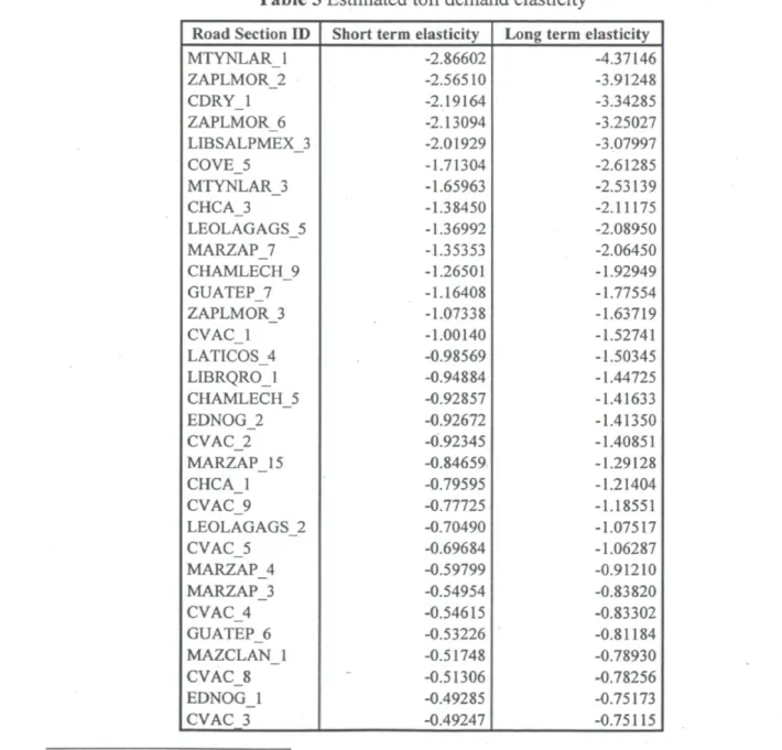
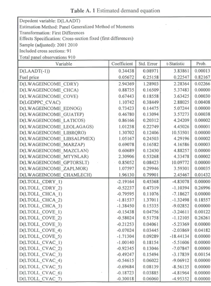
Table 5 shows our toll elasticities results ordered from the highest to the lowest value. These elasticities come from the estimated toll coefficients presented in Table A.l in the

28

Appendix section. Table A.l also displays the full results of our demand equation.

Table 5 Estimated toll demand elasticity

Road Section ID Short term elasticity Long term elasticity

MTYNLARJ -2.86602 -4.37146 ZAPLMOR_2 -2.56510 -3.91248 CDRY_1 -2.19164 -3.34285 ZAPLMOR_6 -2.13094 -3.25027 LIBSALPMEX_3 -2.01929 -3.07997 COVE_5 -1.71304 -2.61285 MTYNLARJ -1.65963 -2.53139 CHCA_3 -1.38450 -2.11175 LEOLAGAGS_5 -1.36992 -2.08950 MARZAP7 -1.35353 -2.06450 CHAMLECH 9 -1.26501 -1.92949 GUATEP7 -1.16408 -1.77554 ZAPLMOR_3 -1.07338 -1.63719 C V A C J -1.00140 -1.52741 LATICOS_4 -0.98569 -1.50345 LIBRQROJ -0.94884 -1.44725 CHAMLECH_5 -0.92857 -1.41633 EDNOG_2 -0.92672 -1.41350 CVAC_2 -0.92345 -1.40851 MARZAP 15 -0.84659 -1.29128 CHCA_1 -0.79595 -1.21404 CVAC_9 -0.77725 -1.18551 LEOLAGAGS_2 -0.70490 -1.07517 CVAC_5 -0.69684 -1.06287 MARZAP_4 -0.59799 -0.91210 MARZAP3 -0.54954 -0.83820 CVAC_4 -0.54615 -0.83302 GUATEP6 -0.53226 -0.81184 MAZCLAN_1 -0.51748 -0.78930 CVAC_8 -0.51306 -0.78256 EDNOG_l -0.49285 -0.75173 CVAC 3 -0.49247 -0.75115

28 The Appendix also reports in Table A.2 the complete name of each toll road segment with its respective

34 GPTORSLT3 -0.48269 -0.73624 LATICOS_3 -0.47902 -0.73063 MAZCLAN2 -0.46352 -0.70700 GUATEP5 -0.45024 -0.68673 LATIC0S_6 -0.44996 -0.68631 GPTORSLT_4 -0.40637 -0.61983 MTYNLAR 2 -0.40414 -0.61643 GUATEP_2 -0.40375 -0.61583 MARZAP12 -0.39698 -0.60550 MARZAP_11 -0.36951 -0.56361 LATICOSJ -0.34114 -0.52033 MARZAP_5 -0.33388 -0.50926 CVAC_10 -0.31800 -0.48504 LATICOS_2 -0.30911 -0.47148 C V A C 7 -0.30018 -0.45786 MARZAP_1 -0.28834 -0.43979 CHAMLECH_13 -0.27743 -0.42316 CHAMLECHJ -0.26913 -0.41049 MARZAP_6 -0.25765 -0.39298 EDNOG_3 -0.25555 -0.38978 MARZAP_9 -0.23916 -0.36479 LIBSALPMEX_1 -0.23246 -0.35457 COVE_3 -0.21253 -0.32416 CVAC_6 -0.18723 -0.28558 EDNOG_5 -0.17552 -0.26771 GUATEP1 -0.17258 -0.26324 COVE_l -0.15438 -0.23547 GUATEP_3 -0.14481 -0.22088 MARZAP_13 -0.13392 -0.20426 GUATEP_4 -0.13285 -0.20263 MARZAP_2 -0.09904 -0.15107 COVE 4 -0.07024 -0.10714 Average -0.71477 -1.09022

Source: Author's own work

Since we choose a log-linear specification for our demand function, the toll coefficients from Table A.l can be used directly as elasticities estimates. However, these should be considered as short term elasticities. In order to obtain long term elasticities we apply the adjustment factor explained in the methodology section to the coefficients.29

35

Also, we exclude from our final elasticity estimates those road sections whose toll coefficients did not exhibit a significance level of at least 10%. That leaves us with 64 of our originally 91 road segments. In absolute terms, 22 of these 64 sections have short run elasticities higher than the average absolute value of 0.71. This means that around one third of this sample has an elastic or nearly unitary elasticity.

Given the relatively high short run average elasticity and the significant proportion of elasticity estimates higher or close to one, Mexican toll road users are more sensitive to tariff changes than the evidence found in the relevant literature. However, this result is not so surprising if we consider the Mexican Constitution legal requirement that every toll road must have a free parallel alternative nearby. Also, some other studies have also found large elasticity estimates. For instance, Odeck and Brâthen (2008) obtained elasticity values as high as -2.26 for their sample of Norwegian tolled road infrastructures.

Another relevant aspect from Table A. 1 is that the fuel price coefficient is not statistically significant. This could be caused by several factors. For instance, as we can see in Table 4 the real average gasoline price in Mexico didn't change much during the observed period. This lack of variability on the fuel price could explain why this variable didn't have a significant impact over the demand for tolled motorways. Specially, if we considered that the demand equation in (5a) was estimated using first differences (i.e. growth rates) after the data transformation required by the AB technique. Also as we mentioned before the fuel price in Mexico is fixed at the national level by the federal government. Therefore, potential toll road users face the same gasoline price no matter which route they choose. Hence, if the toll highway offers time and fuel savings with respect to the free alternative road then is very likely that the fuel price becomes a less relevant component of the generalized travel cost. Under these circumstances, users will probably pay less attention to gasoline prices when making the decision between the toll road and the freeway.

36

Table A. 1 also shows the estimated coefficients for the economic indicators linked to each highway's influence area. All the coefficients present the expected positive sign and are statistically different from zero at the 5% significance level. Furthermore, a Wald test did not accept the null hypothesis that all coefficients are equal, supporting the theory that economic disparities across Mexico's regions are a major factor in explaining toll road demand in the zone of influence of each motorway.

In order to conclude the elasticity analysis, note that we have an ample range of elasticity estimates, as we can see in Table 5, with a minimum short term absolute value of 0.07 and a maximum of 2.86. Therefore, there is a need to explain this wide variation of toll elasticities among road segments. Hence, to address this research objective and following Matas and Raymond (2003) we will perform a series of correlation analysis between the short term elasticity estimates and a group of relevant variables. Fortunately, the specialized literature already gives us several hints on which variables we should include in our analysis. Among others, the explanatory factors most commonly used in other studies are the length of the section (in kilometers), the toll level, and the average speed and the percentage of heavy traffic (i.e. freight trucks) in the alternative road.

We have information for the length of the section, the toll level, the share of freight trucks in the freeway, and the toll as a proportion of the annual average hourly wage in each highway's influential area. However, when we tested the relationship between the short term estimated elasticities and the previous variables we only found a statistically significant negative relationship with the section length and only at the 10% significance level. Therefore we decide to exclude the 5 largest and the 5 lowest elasticities estimates and recalculate the correlations coefficients. With this more compact sample of 54 road sections with an average elasticity of -0.62 we find two correlation coefficients significant at the 95% confidence level. These correlations show a negative relationship of the