Kleshchelski : Washington University in St.Louis, Olin Business School, 1 Brookings Drive, St. Louis, MO 63130
Vincent: HEC Montréal and CIRPÉE, 3000 chemin de la Côte-Sainte-Catherine, Montréal, QC, Canada H3T 2A7
We are especially indebted to Martin Eichenbaum and Sergio Rebelo for their continuous advice. We also thank Torben Andersen, Gadi Barlevi, Marco Bassetto, Craig Burnside, Lars Hansen, Zhiguo He, Ravi Jagannathan, Arvind Krishnamurthy, Jonathan Parker, Giorgio Primiceri, Costis Skiadas, Annette Vissing-Jorgensen, Ernst Schaumburg and seminar participants at Barclays Global Inverstors, Columbia, Duke, Emory, Federal Reserve Bank of Chicago, Federal Reserve Bank of New York, Federal Reserve Board of Governors, Northwestern, UC Berkeley, UCLA, UCSD, University of Houston, University of Minnesota, Washington University.
Cahier de recherche/Working Paper 09-07
Robust Equilibrium Yield Curves
Isaac Kleshchelski Nicolas Vincent
Abstract:
This paper studies the quantitative implications of the interaction between robust control and stochastic volatility for key asset pricing phenomena. We present an equilibrium term structure model in which output growth is conditionally heteroskedastic. The agent does not know the true model of the economy and chooses optimal policies that are robust to model misspecification. The choice of robust policies greatly amplifies the effect of conditional heteroskedasticity in consumption growth, improving the model’s ability to explain asset prices. In a robust control framework, stochastic volatility in consumption growth generates both a state-dependent market price of model uncertainty and a stochastic market price of risk. We estimate the model using data from the bond and equity markets, as well as consumption data. We show that the model is consistent with key empirical regularities that characterize the bond and equity markets. We also characterize empirically the set of models the robust representative agent entertains, and show that this set is “small”. In other words, it is statistically difficult to distinguish between models in this set.
Keywords: Yield curve, market price of uncertainty, robust control
1
Introduction
This paper studies the implications of the interaction between robust control and stochastic volatility for key asset pricing phenomena. We quantitatively show that robustness, or fear of model misspeci…cation, coupled with state-dependent volatility provides an empirically plau-sible characterization of the level and volatility of the equity premium, the risk free rate, and the cross-section of yields on treasury bonds. We also show that robustness o¤ers a novel way of reconciling the shape of the term structure of interest rates with the persistence of yields. Finally, we quantify the level of robustness encoded in agents’behavior.
We construct a continuous-time, Lucas (1978)-type, asset pricing model in which a repre-sentative agent is averse to both risk and ambiguity. The presence of ambiguity stems from the agent’s incomplete information about the economy’s data generating process (DGP). In other words, the agent does not know which of several possible models is the true representation of the economy. Introducing ambiguity aversion into our framework allows us to reinterpret an important fraction of the market price of risk as the market price of model (or Knightian) uncertainty. We model ambiguity aversion using robust control techniques as in Anderson et al. (2003).1 In our model, the representative agent distrusts the reference model and optimally
chooses a distorted DGP. His consumption and portfolio decisions are then based on this dis-torted distribution. Ambiguity aversion gives rise to endogenous pessimistic assessments of the future.
A key assumption in the model is that the output growth process is conditionally het-eroskedastic. The consumption growth process inherits this heteroskedasticity, which gives rise to a stochastic market price of risk. The main contribution of this paper is to show that am-biguity aversion greatly ampli…es the e¤ect of stochastic volatility in consumption growth and, therefore, can explain asset prices in an empirically plausible way. In the absence of ambigu-ity aversion, plausible degrees of stochastic volatilambigu-ity in consumption growth do not generate su¢ cient variation in the stochastic discount factor.
By choosing a distorted DGP, the robust representative agent has biased expectations of fu-ture consumption growth. Being pessimistic, the agent tilts his subjective distribution towards states in which marginal utility is high. With stochastic volatility, positive volatility surges
1Behavioral puzzles such as the Ellsberg paradox (Ellsberg (1961)) led to the axiomatization of the maxmin
decision making by Gilboa and Schmeidler (1989). Robust control is one way of modeling Knightian uncertainty. For a comprehensive treatment of robustness see Hansen and Sargent (2007a). Examples of the use of robust control in economics and …nance include Anderson et al. (2003), Cagetti et al. (2002), Gagliardini et al. (2004), Hansen and Sargent (2007b), Hansen et al. (2006), Liu et al. (2005), Maenhout (2004), Routledge and Zin (2001), Uppal and Wang (2003). An alternative approach to modeling ambiguity allows agents to have multiple priors. See, for example, Epstein and Schneider (2003), Epstein and Wang (1994).
result in a more di¤use distribution of future consumption growth. In that case, the objective distribution assigns more probability mass to future ‘bad’realizations of consumption growth. The agent seeks policies that can reasonably guard against such ‘bad’ realizations. Conse-quently, he increases the distortion to his expectations of consumption growth. The interaction between robustness and stochastic volatility introduces a state dependent distortion to the drift of consumption growth, and therefore, to the drift in the agent’s intertemporal marginal rate of substitution. This state dependent distortion generates sharp implications for asset pricing phenomena.
We estimate our model and assess its implications using data from the equity and bond markets, as well as consumption data. We exploit cross-equation restrictions across bond and equity markets to improve both the identi…cation of structural parameters in our model and the estimation of the market price of risk and uncertainty.2 Our main …ndings are as follows.
First, we show that our model, calibrated with a unitary degree of risk aversion and elasticity of intertemporal substitution (EIS), can reproduce both the high and volatile equity premium and the low and stable risk free rate observed in the data. Previous studies, such as Mehra and Prescott (1985) and Weil (1989), show that explaining the behavior of the equity premium requires implausibly high levels of risk aversion. Ambiguity aversion generates an uncertainty premium that helps to alleviate the di¢ culties encountered in these previous studies. Since there is no benchmark value for the degree of ambiguity aversion, we use detection error probabilities to show that the degree of robustness required to …t the data is reasonable. In other words, we show empirically that the set of models the robust representative agent entertains is small. By this we mean that it is statistically di¢ cult to distinguish between models in this set.
Second, our model can account for the means of the cross-section of bond yields. In partic-ular, we can replicate the upward sloping unconditional yield curve observed in the data. This result highlights a novel interpretation of the uncertainty premium generated by robustness. On empirical grounds, we assume that the conditional variance of output growth, and hence con-sumption growth, is stationary and positively correlated with the concon-sumption growth process. This positive correlation implies that when marginal utility is high the conditional variance of consumption growth is low. Consequently, a downward bias in the subjective conditional
ex-2Campbell (2000) argues that "it is important to reconcile the characterization of the SDF provided by
bond market data with the evidence from stock market data. Term structure models of the SDF are ultimately unsatisfactory unless they can be related to the deeper general-equilibrium structure of the economy. Researchers often calibrate equilibrium models to …t stock market data alone, but this is a mistake because bonds carry equally useful information about the SDF. The short-term real interest rate is closely related to the conditional expected SDF and thus to the expected growth rate of marginal utility; in a representative-agent model with power utility of consumption, this links the real interest rate to expected consumption growth...The risk premium on long-term bonds is also informative."
pectations of consumption growth induces a negative distortion to the subjective expectations of variance changes. We show that this negative distortion is a linear function of the level of the conditional variance process. Consequently, the unconditional distortion is a linear negative function of the objective steady state of the variance process. Therefore, the subjective steady state of the variance process is lower than the objective steady state. In other words, on average, the agent thinks that the conditional variance of consumption growth should decrease. Since the unconditional level of bond yields and the steady state level of the conditional volatility of consumption growth are inversely related, the agent expects, on average, that yields will increase. Consequently, the unconditional yield curve is upward sloping.
Third, our model can replicate the declining term structure of unconditional volatilities of real yields, and the negative correlation between the level and the spread of the real yield curve. The fact that the robust distortion to the conditional variance process is a linear function of the level of the variance implies that the distorted process retains the mean reversion structure of the objective process. Since shocks to the conditional variance are transitory, the short end of the yield curve is more responsive to volatility shocks relative to the long end. Hence, short maturity yields are more volatile than long maturity yields. Also, our model implies that yields are an a¢ ne function of the conditional variance of consumption growth. Therefore, all yields are perfectly positively correlated. Short yields are more responsive to volatility shocks than long yields, but both move in the same direction. So, when yields decrease, the spread between long yields and short yields increases and becomes more positive. As a result, the level and spread of the real yield curve are negatively correlated.
Fourth, the model can reconcile two seemingly contradictory bond market regularities: the strong concavity of the short end of the yield curve and the high degree of serial correlation in bond yields.3 The intuition for this result is closely linked to the mechanism behind the upward sloping real yield curve. Generally, in a one-factor a¢ ne term structure model, the serial correlation of yields is driven by the serial correlation of the state variable implied by the objective DGP. In contrast, in our model the slope of the yield curve is shaped by the degree of mean reversion of the conditional variance process implied by the agent’s distorted (i.e., subjective) distribution. The state dependent distortion to the variance process not only changes the perceived steady state of the variance but also its velocity of reversion. With positive correlation between consumption growth and the conditional variance process, we show that the subjective mean reversion is faster than the objective one. Ex ante, the agent expects shocks to the variance process to die out fast, but ex-post these shocks have a longer lasting
3In a standard one-factor model, it is di¢ cult to separate these two properties, since both observations are
e¤ect than expected. The slope of the yield curve is a re‡ection of how fast the agent expects the e¤ect of variance surges to dissipate. The positive slope of the yield curve declines rapidly when the subjective mean reversion is high. The serial correlation of yields is measured ex-post, using realized yields. If the objective persistence of the variance process is high, yields are highly persistent, which is in line with the empirical evidence. We also show that when the agent seeks more robustness, the separation between the ex-ante and ex-post persistence is stronger.
The remainder of the paper is organized as follows. In section 2 we present our continuous time model and discuss its implications for the equity and bond markets. We derive analytical a¢ ne term structure pricing rules and discuss the distinction between the market price of risk and uncertainty. In sections 3 and 4 we describe our estimation procedure, present the empirical results and explain why our model can match a number of asset pricing stylized facts. We also present independent evidence that supports our modeling assumptions in section 5. We investigate the implied level of uncertainty aversion exhibited by the representative agent in section 6. Finally, we o¤er our concluding remarks and discuss potential avenues for future research in section 7 .
2
Robustness in a Continuous Time Model with
Sto-chastic Volatility
In this section we present an in…nite horizon, continuous time, general equilibrium model in which a robust representative agent derives optimal policies about consumption and invest-ment.4 For simplicity we assume a Lucas tree type economy with a conditionally
heteroskedas-tic growth rate of output. Our ultimate goal is to analyze the implied equilibrium yield curve in this economy and, in particular, identify the implications of robustness for the term structure of interest rates.5
4In the working paper version available at http://neumann.hec.ca/pages/nicolas.vincent/ we present the
robust control idea in a simple two-period asset pricing model.
5Gagliardini et al. (2004) also study the implications of robust control for the behavior of the term structure
of interest rates in a Cox et al. (1985)-type economy. We di¤er from their analysis along two dimensions. First, they study a two factor model closely related to Longsta¤ and Schwartz (1992), while we focus on a one factor model. Second, and more importantly, we study the empirical implications of our model and quantify the contribution of the state dependent market price of model uncertainty to our understanding of asset prices both in the equity and bond market. We also present supporting evidence for our key assumption of state dependent volatility in consumption growth. Finally, we estimate the implied degree of uncertainty aversion implied by the data.
2.1
Reference and Distorted Models
The representative agent in our economy uses a reference or approximating model. However, since he fears that this model is potentially misspeci…ed, he chooses to diverge from it when making his decisions.6 In the context of this paper, the reference model is assumed to generate
the observed data. In contrast with the rational expectations paradigm, the agent entertains alternative DGPs. The size of the set of possible models is implicitly de…ned by a penalty func-tion (relative entropy) incorporated into the agent’s utility funcfunc-tion. So the agent chooses an optimal distorted distribution for the exogenous processes. In other words, the agent optimally chooses his set of beliefs simultaneously with the usual consumption and investment decisions. The robust agent distorts the approximating model in a way that allows him to incorporate fear of model misspeci…cation. We will refer to the optimally chosen model as the distorted model.7
2.2
The Economy
There is a single consumption good which serves as the numeraire. Let D be an exogenous output process that follows a geometric Brownian motion and solves the following stochastic di¤erential equation (SDE),
dDt= Dt dt + DtpvtdBt: (2.1)
The probability measure P on the Brownian process represents the reference or approximat-ing model. However, the agent entertains a set of possible probability measures which size is determined by a penalty function (relative entropy) that is incorporated into the agent’s utility function. We denote the distorted measure which the agent chooses by Q.8 The conditional
expectation operators under P and Q are denoted respectively by Et( )and EQt ( ).
6Another possibility is to claim that for some reason the agent dislikes extreme negative events and wants
to take special precautionary measures against these events. If we choose this behavioral interpretation, we can then assume the agent knows the true DGP, but that his marginal utility function is very high in bad states of the world. Low consumption is so costly that the agent requires policies that are robust to these states. Even though there is complete observational equivalence between the two approaches, they are utterly di¤erent from a behavioral perspective.
7An alternative is to allow for the possibility that a di¤erent, unspeci…ed model, is actually the DGP. In this
scenario, it is likely that neither the distorted nor the reference model generate the data. The agent must in this case infer which model is more likely to generate the data. See Hansen and Sargent (2007b) for an example.
8Formally, we …x a complete probability space ( ; F; P) supporting a univariate Brownian motion B =
fBt: t 0g. The di¤usion of information is described by the …ltration fFtg on ( ; F). All stochastic processes
are assumed to be progressively measurable relative to the augmented …ltration generated by B. The set of possible probability measures on ( ; F) entertained by the agent is denoted by P. Every element in P de…nes the same null events as P. Note that the assumption that the penalty function is the relative entropy imposes a lot of structure on the possible distorted measures. By Girsanov’s theorem we require the distorted measure to be absolutely continuous with respect to the reference measure.
We can obviously think of D as a general dividend process of the economy. We allow the trading of ownership shares of the output tree. The parameters and v are the local expectations (drift) and the local variance of the output growth rate, respectively. We assume that v follows a mean-reverting square-root process:
dvt = (a0+ a1vt) dt +pvt vdBt; (2.2)
a0 > 0; a1 < 0; v 2 R; 2a0 2v:
Note that the same shock (Wiener increments) drives both the output growth and the output growth volatility processes.9 We impose this assumption to retain parsimony. The requirement
a1 < 0 guarantees that v converges back to its steady state level aa01 (= v) at a velocity a1.
The long run level of volatility is positive since a0 > 0. The Feller condition 2a0 2vguarantees
that the drift is su¢ ciently strong to ensure that v > 0 a.e. once v0 > 0. The parameter v is
constant over time and will play an important role in our model.
When v is constant over time, the market price of risk is state independent, and the ex-pectations hypothesis of the term structure of interest rates holds. This result stands in sharp contrast to the empirical evidence (e.g., Fama and Bliss (1987), Campbell and Shiller (1991), Backus et al. (1998), Cochrane and Piazzesi (2002)). We discuss in the next section how sto-chastic volatility interacts with robustness considerations to a¤ect the predictions of our model. Let dRt be the instantaneous return process on the ownership of the output process and St
be the price of ownership at time t. Then, we can write dRt
dSt+ Dtdt
St
(2.3) = R;tdt + R;tdBt;
where R and R are determined in equilibrium. We also let r be the short rate process, which
is determined in equilibrium.
2.3
The Dynamic Program of the Robust Representative Agent
The robust representative agent consumes continuously and invests both in a risk-free and a risky asset. The risky asset corresponds to the ownership of a share of the output process (the tree). The risk free asset is in zero net supply in equilibrium. The agent chooses optimally
9We could also make the expected instantaneous output growth rate, , stochastic. By assuming, for example,
an a¢ ne relation between tand vt, the model remains tractable and can be solved analytically. For the purpose
a distortion to the underlying model in a way that makes his decisions robust to statistically small model misspeci…cation. Formally, the agent has the following objective function
sup C; inf Q E Q t R1 t e (s t)u (C s) ds + Rt(Q) ; (2.4)
subject to his dynamic budget constraint
dWt = rtWt+ tWt R;t rt Ct dt + tWt R;tdBt; (2.5)
where Q is the agent’s subjective distribution, W is the agent’s wealth, is the subjective discount factor, C is the consumption ‡ow process, is the portfolio share invested in the risky asset, and is the multiplier on the relative entropy penalty R. The level of can be interpreted as the magnitude of the desire to be robust. When is set to in…nity, (2.4) converges to the expected time-additive utility case. A lower value of means that the agent is more fearful of model misspeci…cation and thus chooses Q further away from P in the relative entropy sense. In other words, the set of alternative DGPs is larger the smaller is.
Under some regularity conditions and by Girsanov’s theorem, we can de…ne a Brownian motion under Q as
BtQ = Bt
Rt
0hsds; t 0: (2.6)
With this setup at hand, the relative entropy process R (Q) for some Q can be expressed conveniently as10 Rt(Q) = 1 2E Q t R1 t e (s t)h2 sds ; t 0: (2.7) and (2.4) becomes sup C; inf h E Q t R1 t e (s t) u (Cs) + 2h 2 s ds : (2.8)
The change of measure (2.6) also allows us to write (2.1), (2.2) and (2.5) under the distorted measure Q. This introduces a drift distortion, which in the context of the market return has an obvious interpretation: it is the uncertainty premium the agent requires for bearing the risk of potential model misspeci…cation
dRt= 2 4 R;t ( ht R;t) | {z } Uncertainty premium 3 5 dt + R;tdBtQ: (2.9)
The process h is the (negative of the) process for the market price of model uncertainty. The di¤usion part R;t on the return process is, as usual, the risk exposure of the asset. The
product ht R;t is the equilibrium uncertainty premium.11
2.4
Optimal Policies with Robust Control
Let J (Wt; vt)denote the agent’s value function at time t where Wtand vtcorrespond to current
wealth and the conditional variance level respectively.12 One can show that optimal distortion h is given by
ht=
1
(JW;t W;t+ Jv;t vpvt) : (2.10)
A few observations are in order at this point. First, since volatility is stochastic, the ro-bustness correction h is state dependent: the robust agent derives the distorted conditional distribution in such a way that the reference conditional distribution …rst order stochastically dominates the chosen distorted conditional distribution. If it was not the case then there would be states of the world in which the robust agent would be considered optimistic. Also, the agent wants to maintain the optimal relative entropy penalty constant since is constant. In order to achieve this when conditional volatility is stochastic, the distortion has to be stochastic and in-crease with volatility. Second, the size of the distortion is inversely proportional to the penalty parameter : the distortion vanishes as ! 1. Third, whenever the marginal indirect utility and volatility of wealth (JW and W) are high, the agent becomes more sensitive to uncertainty
and distorts the objective distribution more. Low levels of wealth imply large marginal indirect utility of wealth. These are states in which the agent seeks robustness more strongly. The second term in the parentheses corresponds to the e¤ect of the state v on the distortion h. Since Jv < 0 for all reasonable parametrizations, the sign of v dictates the optimal response
of the agent. Consider the benchmark case when v is positive. Following a positive shock,
marginal utility falls as consumption rises, and volatility v increases. Therefore, the investment opportunity set deteriorates exactly when the agent cares less about it. Since the evolution of v serves as a natural hedge for the agent, he reduces the distortion h. The opposite occurs when
v < 0.
Given the choice of a distortion level, the optimal portfolio holding of the risky asset at time t, t, can be expressed in two equivalent forms, each emphasizing a di¤erent aspect of the
11By rewriting the return process under the risk neutral measure, one can also show that there is a perfect
correlation between risk and uncertainty premia in our model.
12See the working paper version at http://neumann.hec.ca/pages/nicolas.vincent/ for a more detailed
deriva-tion of the policies and the value funcderiva-tion. Anderson et al. (2003) and Maenhout (2004) also use similar formulations.
intuition: t = Q R;t rt 2 R;t (2.11) = R;t2 rt R;t + ht R;t :
The …rst line of equation (2.11) states that the demand for the risky asset is myopic: the agent only cares about the current slope of the mean-variance frontier. However, this slope is constructed using his subjective beliefs. From an objective point of view, the agent deviates from the observed mean-variance frontier portfolio due to his (negative) distortion to the mean h: he optimally believes the slope is lower and thus decreases his demand for the risky asset.
We posit the guess that the value function is concave (log) in the agent’s wealth and a¢ ne in the conditional variance, which allows us to rewrite (2.10) as
ht=
1 1
+ 1 v pvt: (2.12)
Here, we see that the distortion, or the (negative of the) market price of model uncertainty is linear in the conditional volatility of the output growth rate. In equilibrium pv is the conditional volatility of the consumption growth rate.
We can also rewrite (2.11) as
t = 1 1 + 1 R;t rt 2 R;t | {z } Myopic demand 1 1 + 1 Jv v | {z } Hedging demand :
The …rst element on the RHS corresponds to a variant of the usual trade-o¤ in a log-utility setup between excess return compensation and units of conditional variance.13 The second element is the hedging-type component arising from uncertainty aversion. It is positive since Jv v > 0 (recall the discussion of (2.10)), and larger in absolute terms the larger Jv or v,
ceteris paribus.
The consumption policy is unchanged when the agent seeks robust policies: C = W . Here, robustness entails that the agent perceives the local expectations on the risky asset to be lower than the objective drift on the same asset. The substitution e¤ect implies that the agent should
13Note that the coe¢ cient is not unitary, as in the usual log problem. The reason is that when introducing
robustness, we e¤ectively increase risk aversion, but maintain the unitary EIS. This pushes down the demand schedule for the risky asset.
invest less since the asset is expected to yield low return in the future. In contrast, the wealth e¤ect predicts that he should consume less today and save instead. In the case of log utility, these two e¤ects cancel each other. Consequently, the e¤ect of robustness on the consumption policy is eliminated. Changing a log-agent’s desire to be robust will only a¤ect the risk free rate and the return on the risk free asset.
2.5
Robust Equilibrium
In this section we solve for the equilibrium prices of assets and discuss the pricing of the term structure of interest rates in our model. First, in our setup a robust equilibrium is de…ned as: De…nition 1 A robust equilibrium is a set of consumption and investment policies/processes (C; ) and a set of prices/processes (S; r) that support the continuous clearing of both the market for the consumption good and the equity market (C = D; = 1) and (2.8) is solved subject to (2.5), (2.2) and (2.6).14
In equilibrium, since the agent consumes the output (C = D) the local consumption growth rate and the local output growth rate are the same ( C = ). Also, the agent’s equilibrium
path of wealth is identical to the evolution of the price of the ‘tree’ since = 1. Therefore, W = S. Hence, D = C = W = S. As is usually the case with a log representative agent, not only the consumption wealth ratio is constant but so is the dividend-price ratio WC = DS = . Consequently, robustness considerations do not a¤ect the consumption policy and the pricing of the ‘tree’. Instead, the implications of uncertainty aversion show up in the risk free rate and the way expectations are formed about growth rates or the return on the risky asset. The equilibrium risk free rate can be derived from (2.11)
rt = + C;t+ pv tht vt = + vt: (2.13) where 1 + 1 1 + 1 v :
As in a standard framework, a larger subjective discount rate or higher future expected consumption growth both make the agent want to save less today and lead to a higher equi-librium real short rate. Also, higher consumption volatility activates a precautionary savings
14The same de…nition also appears in Maenhout (2004). Without stochastic volatility considerations, he also
motive, so that the real rate must be lower to prevent the agent from saving. However, here the presence of implies a role for uncertainty aversion. Intuitively, robustness ampli…es the e¤ect of the precautionary savings motive (h < 0 when <1), and thus lowers the equilibrium level of the short rate. In other words, the robust agent wants to save more than an expected utility agent and therefore needs a stronger equilibrium disincentive to save in the form of lower risk free rate.
The equilibrium local expected return on the risky asset can immediately be derived from (2.3) and the fact that S = D=
dRt = D;t+ dt + D;tdBt
= D;t+ + ht D;t dt + D;tdBtQ:
The observed equity premium is15
R;t rt = vt= |{z}vt Risk Premium + ( 1) vt | {z } Uncertainty Premium = covt dCt Ct ; dRt + 1 1 + 1 v vt:
The equity premium has both a risk premium and an uncertainty premium components. The former is given by the usual relation between the agent’s marginal utility and the return on the risky asset. If the correlation between the agent’s marginal utility and the asset return is negative, the asset commands a positive risk premium
h
covt dCCt
t ; dRt > 0
i
and vice versa. The higher the degree of robustness (i.e., the smaller the parameter ), the larger the uncertainty premium and the market price of model uncertainty. While a decrease in increases the equity premium, it also decreases the risk free rate through the precautionary savings motive. The EIS is independent of .16
15We use the quali…er ‘observed’to emphasize again that what the agent treats as merely a reference model
is actually the DGP. Therefore, anything under the reference measure is what the econometrician observe when he has long time series of data.
16Previous studies (e.g., Anderson et al. (2003), Skiadas (2003), Maenhout (2004)) have shown that when
eliminating wealth e¤ects from robustness considerations, a robust control economy is observationally equivalent to a recursive utility economy in the discrete time case (Epstein and Zin (1989), Weil (1990)) or to a stochastic di¤erential utility (SDU) in the continuous time economy as in Du¢ e and Epstein (1992a) and Du¢ e and Epstein (1992b). Thus, our combined market price of risk and uncertainty can be viewed as an e¤ective market price of risk in the SDU economy. The di¢ culty with such approach is that it requires implausibly high degrees of risk aversion. Another di¢ culty arises in the context of the Ellsberg paradox. Our approach assumes that agents do not necessarily know the physical distribution and want to protect themselves against this uncertainty.
We see that robustness can potentially account for both a high observed equity premium and low level of the risk free rate. What about the volatility of the risk free rate? Since we do not change the substitution motive, the only magni…cation is through the precautionary savings motive. Empirically v is extremely smooth and contributes very little to the volatility of r.17
Next, we need to price the term structure of interest rates, the main object of this study.18 Denote the intertemporal marginal rate of substitution (IMRS) process by where t
e t=C
t. Ito’s lemma allows us to characterize the dynamics of as
d t t
= rtdt pvtdBtQ; (2.14)
where the drift is the (negative of) the short rate and the di¤usion part is the market price of risk. It is then straightforward to price default-free bonds using (2.14). The excess expected return on a bond over the short rate is given by
EQt dpt pt rtdt = d t t dpt pt (2.15) = 1( ) vvt: (2.16)
where the second line follows from our guess of an a¢ ne yield structure, and 1 is positive and
determines the cross section restrictions amongst di¤erent maturity bonds. The excess expected return is determined by the conditional covariance of the return on the bond and marginal utility, or alternatively, by the product of the market price of risk and the risk exposure of the bond. The sign of the risk premium is determined by the correlation of the output growth rate and the conditional variance, v. In times of high volatility, the agent’s decision to shift his
portfolio away from the equity market and towards bonds leads to a rise in bond prices. When
v > 0, this implies that bonds pay well in good times and the risk premium is positive.
Moreover, the observed excess return that long term bonds earn over the short rate is not completely accounted for by the risk premium component. Under the objective measure we
17If we allow for a stochastic with positive correlation with v, ‡uctuations in v will be countered by
movements in since they a¤ect the risk free rate with opposite sign. In other words, if we allow the substitution
e¤ect and the precautionary motive to vary positively over time, the risk free rate can be very stable.
18Our paper belongs to the vast literature on a¢ ne term structure models. The term structure literature is too
large to summarize here but studies can be categorized into two strands - equilibrium and arbitrage free models. Our paper belongs to the former strand. The advantage of the equilibrium term structure models is mainly the ability to give meaningful macroeconomic labels to factors that a¤ect asset prices. Dai and Singleton (2003) and Piazzesi (2003), for example, review in depth the term structure literature.
have, dp ( ; vt) p ( ; vt) = 2 4rt+ 1( ) vvt | {z } Risk Premium + 1( ) vvt( 1) | {z } Uncertainty Premium 3 5 dt + 1( ) vpvtdBt: (2.17)
In the presence of uncertainty aversion, there is an uncertainty premium that drives a wedge between the return on a -maturity bond and the short rate. The more robust the agent, the larger the market price of uncertainty is in absolute terms (i.e., is larger so h = ( 1)pv is larger). Also, higher conditional variance increases the uncertainty premium since the agent distorts the mean of the objective model more. In other words, higher v also increases the
uncertainty exposure of the asset. In section 4 we discuss the intuition behind the predictions of the model, and especially the role robustness plays in our context.
Finally, the yield on a given bond is simply an a¢ ne function of the conditional variance Y ( ; vt) =
1
ln p ( ; vt) :
The two extreme ends of the yield curve are lim !0Y ( ; vt) = rt and lim !1Y ( ; vt) =
+ a0 1. Thus the spread is
lim
!1Y ( ; vt) lim!0Y ( ; vt) = a0 1+ vt;
where 1 is a function of the model parameters.
3
Model Estimation
Since the model permits closed-form expressions for …rst and second moments we use the generalized method of moments (GMM) to estimate our model parameters (Hansen (1982)). Our procedure is similar to the one used by, for example, Chan et al. (1992). Our approach is to exploit mainly the time series restrictions to estimate the structural parameters. We do not focus on the cross sectional restrictions of the model as in Longsta¤ and Schwartz (1992) and Gibbons and Ramaswamy (1993). Since we have a single factor model, yields are perfectly correlated. Therefore, including cross sectional restrictions may reduce the power of the overidentifying restrictions in small samples. We use our point estimates to generate the model’s implied yield curve and compare it to the empirical yield curve. In that sense, our approach is more ambitious. It is important to note that since our model only makes statements about the real economy, all the data we use is denominated in real terms. The description of
the data is relegated to Appendix A.19
We need to estimate 6 parameters fa0; a1; ; ; ; vg. We form orthogonality conditions
implied by the model using the following notation Yt+1 Y (1; vt+1) ; Rt+1; Ct+1 Ct ;Y (4; vt) Y (1; vt) ; Xt Y (1; vt) ; Zt 1;Y (1; vt) ; Rt; Ct Ct 1 ;
where Yt+1 is observed at time t + 1 and contains the change in the one-quarter real yield
( Y (1; vt+1)), the realized real aggregate market return (Rt+1), the realized real aggregate
consumption growth rate Ct+1
Ct and the real spread between the 1-year and 3-months real
yields (Y (4; vt) Y (1; vt)). Xt is the explanatory factor. Even though conditional variance is
not directly observable in the data it is theoretically an a¢ ne function of the short rate (or any other real yield with arbitrary maturity). Therefore, we use the short rate (3-months yield) as an observable that completely characterizes the behavior of the conditional variance. Last, we use lagged 3-months, market return and realized consumption growth rate as instruments in the vector Zt.
The stacked orthogonality conditions are given in m
u1;t+1 Yt+1 Y;tjXt;
u2;t+1 diag u1;t+1u01;t+1 Y;t 0Y;tjXt ;
mt+1
h
u1;t+1 u2;t+1
i Zt:
We draw …rst and second moment restrictions. Y;tjXt and Y;tjXt have the parametric forms
implied by the model and are a¢ ne in Xt.
19A few studies, for example Brown and Schaefer (1994) and Gibbons and Ramaswamy (1993), also use real
data to estimate a term structure model. However, they do not draw restrictions from the equity market and consumption data and their preferences assumption is standard which implies that the equity premium and risk free rate puzzles are still present in the models they estimate.
4
Empirical Results
In this section we …rst present the parameter estimates over various samples before analyzing the empirical …t of our model. We pay particular attention to discussing how the interaction of robust control and stochastic volatility allows us to address a number of asset pricing facts.
4.1
Point Estimates of the Structural Parameters
Table 4.1 presents the point estimates over di¤erent time periods. Aside from the robustness parameter , all coe¢ cients are immediately interpretable. All parameters are statistically di¤erent from zero. Also, the model is not being rejected according to the J-test. We will explain the DEP’s column later.
Table 4.1: Model estimation with consumption volatility over di¤erent time intervals. The data is in quarterly frequency and in quarterly values. 6 parameters are estimated using an iterated GMM. There are 8 moments and 4 instruments that produce 32 orthogonality conditions. T is the number of observation in each estima-tion. Robust t-statistics are indicated below each point estimate. The standard error are corrected using the
Newey-West procedure with 4 lags. p-val is the p-value for the J-test statistic distributed 2 with 26 degrees
of freedom. The DEP column reports the detection error probabilities.
Period T a0 a1 v J-stat/P-val DEP
Q2.52-Q4.06 218 0.0005 -0.1951 0.0052 0.0145 9.5730 0.0189 33.5147 4.41% 6.7904 -10.1242 29.0936 7.6824 3.7579 7.7160 14.77% Q1.62-Q4.06 180 0.0004 -0.1594 0.0051 0.0125 14.9578 0.0175 28.0792 11.01% 6.9588 -10.7284 28.2098 6.3202 2.7028 5.5972 35.46% Q1.72-Q4.06 140 0.0004 -0.1611 0.0048 0.0148 11.8660 0.0149 22.3470 10.86% 6.3636 -10.3456 28.4321 6.1634 2.5565 5.1858 66.96% Q1.82-Q4.06 100 0.0004 -0.1314 0.0054 0.0208 6.6591 0.0082 17.3000 7.31% 6.2872 -6.6014 34.0290 8.7880 3.7862 7.4882 89.97% Q1.90-Q4.06 68 0.0003 -0.0997 0.0050 0.0172 9.0779 0.0064 12.2261 14.49% 8.1423 -9.7387 36.4052 10.5310 5.7235 10.3818 98.98% Q2.52-Q4.81 118 0.0007 -0.2528 0.0050 0.0115 13.4790 0.0431 20.2067 17.11% 7.1360 -13.8242 20.8878 5.6148 2.7839 6.0434 78.17% Q2.52-Q4.89 149 0.0006 -0.2232 0.0053 0.0140 10.6126 0.0290 24.2714 10.10% 6.2481 -9.5348 24.3649 6.3682 3.2241 6.9336 56.04%
Note that both (equal to the average real aggregate quarterly consumption growth rate) and are stable over di¤erent samples.20 What is obvious from Table 4.1 is that the estimation
20In results available from the working paper version, we also estimated the model without imposing the
volatility of consumption growth. What we …nd is that the parameters , , a0 and a1 are mostly una¤ected.
The penalty parameter , however, is higher: without imposing the smooth consumption process , the implied pricing kernel (SDF) is much more volatile and less robustness is needed to justify the observed asset prices.
procedure detects mostly high frequency movements and not the slow moving component in consumption growth volatility identi…ed by Bansal and Yaron (2004). Hence, it appears that the high-frequency component from the market data dominates in the full-model estimation. We will discuss further our parameter estimates in the context of the …t of the model.
4.2
Theoretical and Empirical Moments
Table 4.2 presents a comparison of model-implied and empirical moments over di¤erent time spans for the main focus of our study, the bond market. In general, the model fares very well: it can generate average bond yields very similar to those in the data. In addition, it is able to …t the autocorrelation of yields as well as the return from a strategy of holding a one-year bond for three quarters.
Table 4.2: Empirical and theoretical bond market moments (with consumption volatility restriction). The period column represents the time interval of the data that is used to estimate the model. The data is in quarterly frequency with quarterly values. T is the number of quarterly observations used to estimate the model. Columns with the number (1) present the empirical moments. Empirical moments computed with the data and theoretical moments are implied by the estimated model. Columns with the number (2) present the theoretical moments. The theoretical moments were generated using 1; 000 replications of the economy that was calibrated using the estimated parameters over the corresponding period. Robust standard errors are given below each moment. The standard errors were corrected using the Newey-West procedure with 4 lags. The standard errors for the theoretical moments were computed over the 1; 000 replications. All moments,
aside from the autocorrelations, are given in % values. Y3m, Y1y, and (Y3m) are the real 3 month yield, real
1 year yield and the …rst order autocorrelation coe¢ cient of the real 3 month yield, respectively. The last column reports real holding period return for buying a one year to maturity bond and selling it after three quarters. Period T Y3m Y1y (Y3m) ln h p(1;vt+3) p(4;vt) i (1) (2) (1) (2) (1) (2) (1) (2) Q2:52 Q4:06 218 1.531 1.838 2.250 2.570 0.843 0.863 2.465 2.802 0.263 0.083 0.234 0.055 0.060 0.004 0.274 0.047 Q1:62 Q4:06 180 1.749 2.191 2.241 2.614 0.835 0.878 2.394 2.750 0.292 0.011 0.279 0.008 0.071 0.000 0.321 0.007 Q1:72 Q4:06 140 1.686 2.216 2.214 2.680 0.830 0.875 2.359 2.847 0.362 0.080 0.351 0.058 0.075 0.004 0.406 0.047 Q1:82 Q4:06 100 2.190 2.584 2.742 3.071 0.862 0.891 2.932 3.232 0.366 0.109 0.378 0.084 0.062 0.003 0.443 0.073 Q1:90 Q4:06 68 1.666 1.914 2.015 2.233 0.897 0.890 2.118 2.346 0.422 0.135 0.371 0.111 0.058 0.006 0.420 0.110 Q2:52 Q4:81 118 0.965 1.572 1.865 2.471 0.804 0.784 1.976 2.764 0.330 0.210 0.247 0.118 0.096 0.010 0.275 0.090 Q2:52 Q4:89 149 1.469 2.207 2.358 2.996 0.823 0.825 2.586 3.257 0.328 0.143 0.292 0.088 0.077 0.007 0.348 0.070
Table 4.3 shows some key moments for the equity and consumption data. While the model-implied moments are comparable to their empirical counterparts, in fact we may say that our model is performing too well: it generates an equity premium larger than in the data, while still matching the low consumption growth rate as well as the bond market facts. The same conclusion seems to hold over di¤erent time horizons. Note, however, that since we are imposing consumption growth volatility, the model compromises on the implied market return volatility being somewhere between the empirical consumption growth rate volatility and the empirical market return volatility.21
Table 4.3: Empirical and theoretical equity and goods market moments (with consumption volatility restric-tion). The period column represents the time interval of the data that is used to estimate the model. The data is in quarterly frequency with quarterly values. T is the number of quarterly observations used to esti-mate the model. Columns with the number (1) present the empirical moments. Empirical moments computed with the data and theoretical moments are implied by the estimated model. Columns with the number (2) present the theoretical moments. The theoretical moments were generated using 1; 000 replications of the economy that was calibrated using the estimated parameters over the corresponding period. Robust standard errors are given below each moment. The standard errors were corrected using the Newey-West procedure with 4 lags. The standard errors for the theoretical moments were computed over the 1; 000 replications. All
moments are given in % values. R, C, R, and Y3mare the real return on the market (including dividends),
real growth rate of consumption, volatility of real aggregate market return and real 3 month yield, respec-tively. Period T R R Y3m R C (1) (2) (1) (2) (1) (2) (1) (2) Q2:52 Q4:06 218 8.690 12.346 7.069 10.354 16.445 9.861 2.096 2.099 1.120 0.078 1.133 0.118 1.112 0.081 0.086 0.075 Q1:62 Q4:06 180 7.440 10.589 5.606 8.245 17.092 9.708 2.074 1.526 1.233 0.111 1.239 0.160 1.254 0.172 0.093 0.110 Q1:72 Q4:06 140 7.973 11.023 6.198 8.645 17.418 10.224 1.927 1.524 1.456 0.093 1.457 0.132 1.440 0.111 0.101 0.092 Q1:82 Q4:06 100 11.159 12.294 8.807 9.501 16.579 10.507 2.199 1.588 1.544 0.151 1.532 0.204 1.478 0.168 0.088 0.152 Q1:90 Q4:06 68 9.110 10.033 7.342 7.991 15.984 10.068 2.028 1.349 1.920 0.178 1.894 0.241 1.841 0.136 0.100 0.176 Q2:52 Q4:81 118 6.787 15.933 5.777 14.187 16.223 9.901 1.988 1.802 1.541 0.152 1.592 0.256 1.624 0.300 0.138 0.141 Q2:52 Q4:89 149 8.498 14.082 6.944 11.665 16.653 9.897 2.128 1.826 1.388 0.117 1.418 0.188 1.379 0.199 0.116 0.114
Next, we provide intuition about the role of robustness in matching bond market moments.
21We also tried to reestimate the model without imposing consumption growth volatility. The results were
qualitatively similar. Not surprisingly, this version was better able to match the aggregate market return volatility, at the expense of higher consumption growth rates. Results for the yield curve were however relatively unchanged.
4.2.1 Bond Returns and Upward Sloping Yield Curve
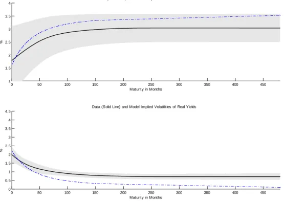
Results for the 3-months and 1-year real yields reveal that the model is doing a good job at reproducing the shape of the short end of the yield curve. To get a better idea of its ability to replicate the term structure of interest rates, the top panel in Figure 4.1 presents estimation results over the years 1997 2006. During this period TIPS bonds were traded in the U.S. and thus provide a good proxy to real yields. The solid line is the average level of the yield curve over this period with 95% con…dence bands. The dot-dashed line is the model-implied average yield curve. Note that we only impose two bond market restrictions in the estimation procedure and yet the model can imitate reasonably well the shape of the entire yield curve.
0 50 100 150 200 250 300 350 400 450 1 1.5 2 2.5 3 3.5 4
Data (Solid Line) and Model Implied Real Yield Curves
% Maturity in Months 0 50 100 150 200 250 300 350 400 450 0 0.5 1 1.5 2 2.5 3 3.5 4 4.5
Data (Solid Line) and Model Implied Volatilities of Real Yields
%
Maturity in Months
Figure 4.1: Top panel: average real yield curve extracted from the TIPS data from M 1:97 M 12:06 (solid
line) with 95% con…dence bands with Newey-West (12 lags) correction. Model implied average yield curve (dot-dashed line). The model is estimated over the same period as the empirical yield curve. Bottom panel: empirical term structure of unconditional volatilities of the TIPS data (solid line). with 95% con…dence bands with Newey-West (12 lags) correction. The model is estimated over the same period as the empirical yield curve.
Two elements allow our model to match the term structure of interest rates. First, recall from expression (2.17) that robustness introduces an uncertainty premium in addition to the usual risk premium through the precautionary savings motive. Both premia are positive as long
as v > 0, (i.e. shocks to consumption growth and volatility are positively correlated). The
magnifying role of robustness means that one can match the excess return on long term bonds relative to short term bonds with a moderate amount of stochastic volatility.
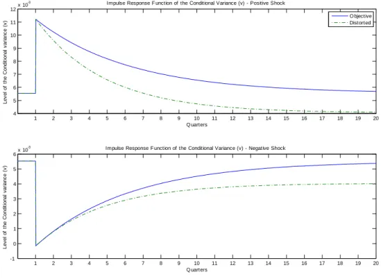
Second, with robustness the (perceived) evolution of v under the distorted measure Q is di¤erent from the evolution of v under the objective measure P in two respects. In Figure 4.2 we plot the objective and perceived impulse response functions for the conditional variance v following a shock. Note that, unlike a rational expectations agent, the robust agent is on average wrong about the future evolution of v: uncertainty aversion leads him to distort his beliefs such that, on average, he expects the conditional variance to decrease over time.22 In
Section 6 we argue that this bias is not statistically unreasonable. This observation provides an additional channel for an upward-sloping yield curve: through the precautionary savings motive, lower future volatility results in higher expected yields.
Another manifestation of the forces just described is apparent in the last column of Table 4.3. It captures the return of a strategy in which the agent buys a 1-year bond and sells it after 3 quarters. Backus et al. (1989) point to the di¢ culty of representative agent models to account for both the sign and magnitude of holding period returns in the bond market. Note that we did not impose any holding period returns conditions in the estimation procedure and yet the model captures the returns dynamics well.
The bottom panel of Figure 4.1 depicts the term structure of the volatilities of yields. Clearly, the model can replicate the downward slope due to the mean reversion in the estimated conditional variance process, as discussed earlier. The impression is that the procedure anchors the implied …rst and second moments of the 1-year yield to its empirical counterpart, but it is still doing a good job in approximating the entire curve.
22To see this algebraically, write (2.2) under both measures
dvt = v(vt v) dt + vpvtdBt
= Qv vt vQ dt + vpvtdBtQ: (4.1)
Here, v is the velocity of reversion and v is the steady state of v, both under the reference measure. However,
the subjective velocity of reversion is
Q
v = v v(1 ) > v (4.2)
and the subjective steady state is
vQ= v
Q v
v < v: (4.3)
1 2 3 4 5 6 7 8 9 10 11 12 13 14 15 16 17 18 19 20 4 5 6 7 8 9 10 11 12x 10 -3 Q uarters L ev el of t h e C o nd it ional v a ri a nc e (v )
Impulse Response F unction of the Conditional Variance (v) - Positive Shock
O bjective Distorted 1 2 3 4 5 6 7 8 9 10 11 12 13 14 15 16 17 18 19 20 -1 0 1 2 3 4 5 6x 10
-3 Impulse Response F unction of the Conditional Variance (v) - Negative Shock
Q uarters L ev el of t h e C o nd it ional v a ri a nc e (v )
Figure 4.2: Biased expectations. Using the parameters estimated over the entire period Q2:52 Q4:06, the
…gure shows the impulse response function of the conditional variance to a positive and negative shocks. The solid line represents the objective evolution of v and the dashed line represents what the robust agent believes the evolution of v is going to be.
4.2.2 Slope of the Yield Curve and Persistence of Yields
Traditionally, one-factor models encounter an inherent di¢ culty in trying to account simultane-ously for the rapidly declining slope of the yield curve (i.e., strong convexity of the slope of the yield curve) and the high persistence of yields. Time-series evidence implies that interest-rate shocks die out much more slowly than what is implied from the rapidly declining slope of the average yield curve (Gibbons and Ramaswamy (1993)).
Even though we present a one-factor model, we can account for these two facts with a single parametrization. Figure 4.1 shows that the agent prices the yield curve as if shocks to v die out fast. However, Table 4.2 con…rms that the model can still match the persistence of the short rate ( (Y3m)).23
23The term structure literature usually identi…es 3 factors that account well for most of the variation in the
yield curve (Litterman and Scheinkman (1991)): level, slope and curvature. The level slope is very persistent and, thus, accounts for most of the observed persistence of yields. Also, note that we do not impose this restriction in our estimation and yet the model is able to match this moment with high accuracy.
The key for understanding the success of our model on that dimension lies in expression (4.2). The agent believes that the conditional variance reverts to its steady state faster than under the objective measure Q
v > v . Since yields are a¢ ne functions of the conditional
variance of consumption growth, they inherit the velocity of reversion of v under the objective model. In other words, the persistence of yields is measured ex-post and is solely determined by the objective evolution of v without any regard to what the agent actually believes.
At the same time, the slope of the yield curve (or the pricing of bonds) is completely determined by what the agent believes the evolution of v will be, as discussed earlier. If Q
v is
substantially larger than v, the slope of the yield curve can ‡atten at relatively short horizons,
re‡ecting the beliefs of the agent that v will quickly revert to its steady state level. Since the agent persistently thinks that Q
v > v the slope can be on average rapidly declining.
4.2.3 Spread and Level of Yields
In quarterly data over the sample 52:Q2 06:Q4 the correlation between the level and slope of the real yield curve is 0:5083 with standard errors of 0:0992 (where the slope is the di¤erence between the 1-year and 3-months yields). This …nding is robust over di¤erent time intervals and di¤erent frequencies. The model can account for this fact in the following way24: recall
that a positive shock to conditional volatility lowers yields. Also note that yields are perfectly (positively) correlated since all of them are an a¢ ne function of the same factor. However, short yields are more sensitive to conditional volatility shocks. To understand why, it helps to think about the mean reversion of the conditional variance (the ergodicity of its distribution). The e¤ect of any shock is expected to be transitory. The full impact of the shock happens at impact and then the conditional variance starts reverting back to its steady state. Therefore, the e¤ect of, say, a positive shock is expected to dissipate and yields are expected to start to climb back up. This expected e¤ect is incorporated into long term yields immediately. Short yields in the far future are almost una¤ected by the current shock since it is expected that the e¤ect of the shock will disappear eventually. Since long term yields are an average of future expected short yields plus expected risk premia, they tend to be smoother than short term yields.
The expected risk premium is also a linear function of the state, and thus inherits its mean reversion. Therefore, the expected risk premium in the far future is also smoother than the risk premium in the short run. This also contributes to the rotation of the yield curve: since the
24We explain the intuition through the time variation of the conditional volatility of consumption growth
rate. One can alternatively use the substitution channel and focus on time variation in expected consumption growth rate.
short end of the yield curve is very volatile relative to the long end (recall Figure 4.2), whenever yields decrease, the spread increases (or become less negative, depending on the initial state). The opposite also holds true.
5
Additional Evidence
The success of our model in replicating numerous moments for both the equity and bond markets rests on two ingredients: (1) state-dependent volatility of consumption growth, and (2) a positive correlation between shocks to consumption growth and volatility ( v > 0). In this
subsection we provide direct empirical evidence about the level and behavior of the conditional variance of real aggregate consumption growth.
5.1
ARMAX-GARCH Real Consumption Growth Rate
We start with a simple univariate time series parametric estimation. The model we are …tting to the consumption growth process is an ARMAX(2; 2; 1) model and a GARCH(1; 1) to the innovations process: A (L) Ct Ct 1 = c + B (L) Rt 1+ C (L) C;t; (5.1) C;t+1 = C;t"C;t+1; "C;t N (0; 1) ; D (L) C;t = ! + F (L) 2C;t;
where A; B; C; D; F are polynomials of orders 2; 1; 2; 1; 1 respectively, in lag operators. Ct
Ct 1, Rt,
t are, respectively, the realized real consumption growth rate at time t, the real return on the
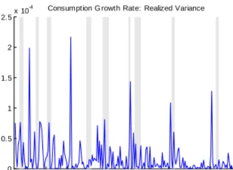
aggregate market index at time t 1, and an innovation process with time-varying variance. In Figure 5.1 we plot the GARCH volatility estimates for both real aggregate consumption growth rate and the real return on the aggregate stock market. We also plot a measure of realized volatility for both consumption growth and market return series that we obtain by …tting an ARMA(2; 2) to the original data and then use the square innovations to construct the realized variance series. The sample period is Q2:52 Q4:06.
First, there seems to be evidence of what has been dubbed as the ‘Great Moderation’(e.g., Stock and Watson (2003)). It is clear that consumption growth volatility has slowly declined over the sample period but the volatility of the market return did not. This pattern is apparent in both measures of conditional volatility.
1955 1960 1965 1970 1975 1980 1985 1990 1995 2000 2005 1
1.5 2 2.5x 10
-5 Consumption G rowth Rate: G ARCH(1,1)
1955 1960 1965 1970 1975 1980 1985 1990 1995 2000 2005 0 0.5 1 1.5 2 2.5x 10
-4 Consumption G rowth Rate: Realized Variance
1955 1960 1965 1970 1975 1980 1985 1990 1995 2000 2005 0 0.005 0.01 0.015 0.02 0.025 0.03 0.035
Real Market Return: G ARCH(1,1)
1955 1960 1965 1970 1975 1980 1985 1990 1995 2000 2005 0 0.02 0.04 0.06 0.08 0.1
Real Market Return: Realized Variance
Figure 5.1: ARMAX-GARCH estimation for both real consumption growth rate and real aggregate market return. We …t model (5.1) and present the GARCH estimates for the conditional variance of real consumption growth rate and real aggregate market return in the left panel. The right panel present the square innovations from an ARMX speci…cation to real consumption growth and real aggregate market return. The quarterly
data is Q2:52 Q4:06. The gray bars are contraction periods determined by the NBER.
a very low frequency stochastic trend in consumption growth volatility. Panel A of Table 5.1 presents the implied reversion coe¢ cient and half life derived using the autoregressive coe¢ cient from the GARCH estimated conditional variance series.25 For comparison purposes, Panel A of
Table 5.1 presents the half life of the volatility shock process implied by our earlier estimation results. We also present in that panel the perceived half life by the robust agent. Expression (4.2) shows that the perceived velocity of mean reversion is faster than the physical speed at which shocks to volatility die out. In general, the point estimates imply that shocks to volatility die out relatively fast. These results con…rm that without forcing asset market restrictions on the consumption series, we observe a very slow moving process for conditional variance. At the same time, the conditional variance of the aggregate market return is much less persistent. The
25Our point estimates correspond to quarterly data. In general, with data sampled at quarterly frequency one
can map an autoregressive coe¢ cient to a coe¢ cient governing the speed of reversion as our v. Let ^ denote
the autoregressive coe¢ cient. Then, the quarterly speed of reversion coe¢ cient v = ln (^) and the half life
general estimation procedure results in panel A are, to some extent, a combination of these two e¤ects.26
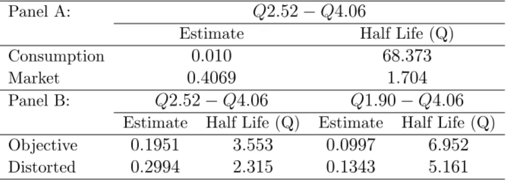
Table 5.1: Panel A: Point estimates of the velocity of reversion coe¢ cient and the implied half life (in quar-ters) of the conditional variance process. Objective referes to the physical rate in which the conditional vari-ance gravitates to its steady state. Distorted referes to the rate in which the robust agent believes the condi-tional variance gravitates to its steady state. These point estimates are from the estimation procedure that imposes the volatility of real aggregate consumption growth rate as a moment condition. Panel B: implied reversion coe¢ cients and half lifes (in quarters) for the conditional volatility of consumption growth rate and aggregate market return derived from the GARCH procedure. The consumption growth rate mean is modeled as an ARMAX(2,2,1) and the aggregate market return is modeled as ARMA(2,2).
Panel A: Q2:52 Q4:06
Estimate Half Life (Q)
Consumption 0:010 68:373
Market 0:4069 1:704
Panel B: Q2:52 Q4:06 Q1:90 Q4:06
Estimate Half Life (Q) Estimate Half Life (Q)
Objective 0:1951 3:553 0:0997 6:952
Distorted 0:2994 2:315 0:1343 5:161
The recent ‘long run risks’literature usually calibrates asset pricing models with a highly persistent conditional variance process.27 For example, Bansal and Yaron (2004) assume that
the autoregressive coe¢ cient (with monthly frequency data) in the conditional variance of the consumption growth process is 0:987.28 This number implies a half life of 13:24 quarters, which
is almost 4 times higher than the number we obtain in our empirical results. As explained earlier, this di¤erence is driven largely by the inclusion of equity and bond markets in our set of moments. What we show in this paper is that robust decision making coupled with state dependent volatility requires moderate levels of persistence in the conditional variance of the consumption growth process. Recall that we assume a constant drift in consumption growth. If we assume a stochastic and highly persistent , as in Bansal and Yaron (2004), we would need to worry about the volatility of the risk free rate. In other words, if the substitution e¤ect channel is very persistent and the precautionary savings motive is much less persistent, the
26We conduct this comparison only for the entire period Q2:52 Q4:06 since we want to examine evidence
concerning very low frequency components. Even our longest sample is somewhat short to conveniently detect the slow moving component. We believe that shorter samples will make the detection exercise impossible.
27Bansal and Yaron (2004) …nd that introducing a small highly persistent predictable component in
consump-tion growth can attenuate the high risk aversion implicaconsump-tions of standard asset pricing models with recursive utility preferences. However, this persistent component is di¢ cult to detect in the data. Croce et al. (2006) present a limited information economy where agents face a signal extraction problem. Their model addresses the identi…cation issues of the long run risk component. Hansen and Sargent (2007b) is another example for the di¢ culty in identifying the long run risk component. However, in addition to a signal extraction problem, their agent seeks robust policies and consequently his estimation procedure is modi…ed.
short rate can potentially be very volatile. If shocks to were to die out much slower than shocks to v, the ergodic distribution of the short rate would be very volatile. In that sense, we might be able to reconcile our results with the calibration exercise of Bansal and Yaron (2004) if we assumed an expected consumption growth rate process.
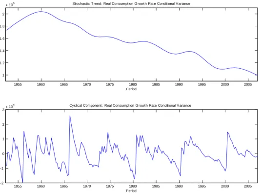
Our hypothesis is that higher frequency ‡uctuations are channeled through the asset market while there are other aspects which we do not identify that contribute to the low frequency ‡uctuations. In other words, when we estimate the full model, the e¤ect of the equity and bond market restrictions is re‡ected in the implied persistency of the conditional variance process. Here, we use the Hodrick-Prescott …lter with parameter 1600 to disentangle these two components of consumption growth volatility. Figure 5.2 presents this result and makes clear that the decline in the low frequency component started in the 060, before the Great
Moderation.29
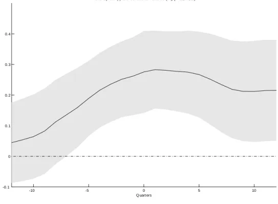
We also use the volatility estimates to explain asset prices (see also Chapman (1997), Bansal and Yaron (2004), Bansal et al. (2005)). In particular, in …gure 5.3 we examine the dynamic cross correlation patterns between consumption growth volatility obtained from the GARCH estimation in (5.1) and the spread between the real 1-year real yield and the real 3-months real yield.
These patterns agree with the model’s predictions. We know that shorter maturity yields respond more than longer maturity yields to a volatility shock. This result is mainly due to the ergodicity of the state variable that a¤ect yields. If the state is assumed to revert back to a known steady state, we expect the longer yield to have a smaller response to contemporaneous shocks. Note that we do not identify the type of shock in this exercise. We merely observe a shock that happens to a¤ect both consumption growth volatility and the bond market.
The second result is the sign response of the yields to a volatility shock. When conditional volatility increases we see that yields decrease. From the precautionary savings motive e¤ect
29In our model it is hard to make ‘conditional’statements about the economy, mainly because we modeled a
constant drift to the consumption growth rate process. It is obviously interesting to think about the correlation structure of expected consumption growth rate and the conditional variance process. Empirically, there is evidence that suggests that interest rates are procyclical (e.g., Donaldson et al. (1990)) and volatility is either countercyclical or at least slightly leads expected growth rates which are believed to be countercyclical (e.g., Whitelaw (1994)). Our conditional variance process is assumed to correlate positively with realized consumption growth rate. Also, the conditional variance correlate negatively with interest rates. In this sense, variance and real interest rates behave as in the data. If, for example, expected growth rate correlate negatively with realized consumption growth rates, they will correlate negatively with the conditional variance. In that case, a positive shock to consumption growth rate will have a double negative e¤ects on real interest rates. Expected growth rates will be low and thus the substitution e¤ect will make equilibrium real interest rates lower. At the same time, conditional variance will be higher and the precautionary savings motive will push the equilibrium real interest rate even lower. Also, Chapman (1997) documented the strong positive correlation of real yields and
1955 1960 1965 1970 1975 1980 1985 1990 1995 2000 2005 1 1.2 1.4 1.6 1.8 2
x 10-5 Stochastic T rend: Real Consumption G rowth Rat e Conditional Variance
Period 1955 1960 1965 1970 1975 1980 1985 1990 1995 2000 2005 -2 -1 0 1 2 3x 10
-6 Cyclical Component: Real Consumption G rowth Rate Conditional Variance
Period
Figure 5.2: HP-‡itered conditional variance of real consumption growth rate derived from an ARMAX-GARCH estimation in (5.1). The top panel presents the low frequency trend and bottom panel presents the
cyclical component. The HP-…lter parameter is 1600. The quarterly data is over the period Q2:52 Q4 06.
we do expect such response. Since in our model ambiguity aversion ampli…es the precautionary savings motive, we expect this channel to play an important role when linking consumption growth volatility and yields. When combining these two results, we expect the spread to increase with a volatility shock. In other words, on average, the yield curve rotates when a shock to volatility occurs.
There are three caveats to these results. First, the upper left panel in Figure 5.1 depicts the behavior of the conditional variance of real consumption growth. One can argue that the series exhibit a non-stationary behavior. If this is the case, then the GARCH process is potentially misspeci…ed. Given the slow-moving component we identi…ed, it is hard to convincingly argue against such hypothesis. Second, our macro data is sampled at quarterly frequency. Drost and Nijman (1993) have shown that temporal aggregation impedes our ability to detect GARCH e¤ects in the data. Even if our model is not misspeci…ed, the fairly low frequency sampling may suggest it is (see also Bansal and Yaron (2004)). Third, we showed that the (sign of the) correlation between shocks to realized consumption growth and the conditional variance
-10 -5 0 5 10 -0.1 0 0.1 0.2 0.3 0.4
Yields Spread (t) and Conditional Variance (t+ j, j= -12,..., 12)
Q uarters C o rr elat ion
Figure 5.3: Dynamic cross-correlation between real consumption growth rate volatility and the real spread
between the 1 year and 3 months yields. The quarterly data covers the period Q2:52 Q4:06.
is important in explaining risk and uncertainty premia. The simple GARCH exercise does not help us identify the sign of this correlation. We address this di¢ culty next.
5.2
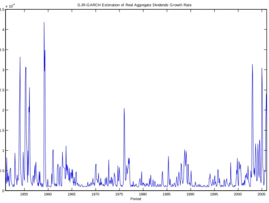
Real Dividends Growth Rate: GJR-GARCH
Since we argue that the sign of v plays an important role in understanding risk premia in our
model, we also estimate a GJR-GARCH(1; 1) (Glosten et al. (1993)). Originally, this model was constructed to capture ‘leverage’ e¤ects when examining market returns (i.e., a negative shock to returns means lower prices and more leveraged …rms, hence higher volatility of future returns). Here we use it with a di¤erent interpretation in mind. We use the leverage coe¢ cient to extract information about the sign of the correlation between consumption/dividends growth rate innovations and conditional variance innovations. Since we argue that the sign of v is
positive, as indicated by asset prices behavior, we hope to …nd the reverse of a leverage e¤ect.30
30Even though our interpretation has nothing to do with the leverage e¤ect discussed in Glosten et al. (1993),


![[PDF] Cours Langages de Programmation Caml | Formation informatique](data:image/gif;base64,R0lGODlhAQABAIAAAP///wAAACH5BAEAAAAALAAAAAABAAEAAAICRAEAOw==)