Slip length measurement of gas flow

HAL Id: hal-01392553

https://hal.archives-ouvertes.fr/hal-01392553

Submitted on 4 Nov 2016

HAL is a multi-disciplinary open access

archive for the deposit and dissemination of

sci-entific research documents, whether they are

pub-lished or not. The documents may come from

teaching and research institutions in France or

abroad, or from public or private research centers.

L’archive ouverte pluridisciplinaire HAL, est

destinée au dépôt et à la diffusion de documents

scientifiques de niveau recherche, publiés ou non,

émanant des établissements d’enseignement et de

recherche français ou étrangers, des laboratoires

publics ou privés.

Distributed under a Creative Commons Attribution - ShareAlike| 4.0 International

Slip length measurement of gas flow

Abdelhamid Maali, Stéphane Colin, Bharat Bhushan

To cite this version:

Abdelhamid Maali, Stéphane Colin, Bharat Bhushan. Slip length measurement of gas flow.

Nan-otechnology, Institute of Physics, 2016, 27 (37), pp.374004. �10.1088/0957-4484/27/37/374004�.

�hal-01392553�

Slip length measurement of gas

flow

Abdelhamid Maali

, Stéphane Colin

and Bharat Bhushan

1

Univ. Bordeaux, LOMA, UMR 5798, F 33400 Talence, France

2

CNRS, LOMA, UMR 5798, F 33400 Talence, France

3

Institut Clément Ader(ICA), Université de Toulouse, CNRS INSA ISAE Mines Albi UPS, Toulouse France

4

Nanoprobe Laboratory for Bio & Nanotechnology and Biomimetics, Ohio State University, 201 W 19th Avenue, Columbus, OH 43210 1142, USA

E mail:bhushan.2@osu.edu

Abstract

In this paper, we present a review of the most important techniques used to measure the slip length of gasflow on isothermal surfaces. First, we present the famous Millikan experiment and then the rotating cylinder and spinning rotor gauge methods. Then, we describe the gasflow rate experiment, which is the most widely used technique to probe a confined gas and measure the slip. Finally, we present a promising technique using an atomic force microscope introduced recently to study the behavior of nanoscale confined gas.

Keywords: slip length, gasflow, confined gas, Millikan experiment, atomic force microscopy

1. Introduction

Understanding the physics of fluid flows at the micro- and nanoscale is crucial for designing, fabricating, and optimizing micro- and nano-electro-mechanical systems (MEMS/ NEMS). The large surface-to-volume ratio of MEMS/NEMS enables factors related to surface effects to dominate thefluid flow physics from the micro- to the nanoscale.

Fluid flow close to solid surfaces has been studied in detail in the last century[1 16]. In gases, due to local

ther-modynamic non-equilibrium, the velocity profile exhibits a phenomenon known as slip, which means that the fluid velocity near the solid surface is not equal to the velocity of the solid surface. The existence of slip in gasflows was first predicted by Maxwell[16] and its magnitude depends on the

degree of rarefaction of the gas. To describe this degree of rarefaction, the Knudsen number, Kn=l D, has been

introduced. It compares the mean free path l of the gas molecules and a characteristic length D of theflow domain, for example the hydraulic diameter of a duct. When the Knudsen number is on the order of 0.001 or larger, the rar-efaction of the gas has to be taken into account, and a non-negligible slip occurs on the surfaces[7 9,12,13]. The slip

velocity has been initially modeled by Maxwell slip

conditions for an isothermal wall as

= ¶ ¶ ₌ V b V z . 1 s z 0 ( )

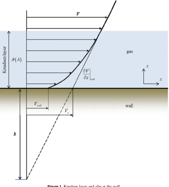
In this equation, b is the slip length. Maxwell proposed its form as b =l(2 -s s) where σ is a coefficient that represents the fraction of the gas molecules that are reflected diffusively from the solid surface atz=0, assuming that the complementary fraction of the molecules is reflected spec-ularly. The so-called slip velocity Vs is different from the actual macroscopic velocity of the gas at the wall: it is linearly extrapolated from the velocity profile outside the Knudsen layer(see figure1), which is a very thin layer of gas in local

thermal non-equilibrium state, where the usual Navier Stokes equations are not valid. The thickness of this layer is of the same order of magnitude as the mean free pathλ. The initial expression (1) of the velocity slip provided by Maxwell, which is in a dimensionless form of thefirst order in Kn, has further been discussed by numerous researchers, and various improved slip boundary conditions, including corrective coefficients and higher orders, have been proposed tentatively in the literature[17]. Unfortunately, there is currently no clear

consensus for recommending the most appropriate equation and corrective coefficients for this slip boundary condition. In

addition, there is often a confusion between s and the tan-gential momentum accommodation coefficient st [18]. The values of the coefficients s and stare also generally not well known.

Consequently, in order to discuss the accuracy and the limits of applicability of the boundary conditions proposed in the literature, there is a crucial need of smart experimental data on slip length in rarefied gas flows. In this paper, we review all techniques used to measure the slip length and the accommodation coefficient in a gas flow on isothermal sur-faces. The paper is divided into five main sections. In section2, the Millikan experiment is presented. In section3, the rotating body techniques(rotating cylinder and spinning rotor gauge methods) are presented. Section 4 is devoted to massflow rate measurements and velocimetry in micro- and nano-channels. In section 5, experimental results using an atomic force microscope(AFM) are shown. Finally, conclu-sions and the outlook for this research area are provided in section6.

2. Millikan’s droplet experiment

Millikan has introduced the concept of gas slip to explain the results of his famous experiment on electron charge mea-surement [2, 19 21]. His experiment consists of measuring

the terminal velocities v1and v2of a spherical charged droplet

in two consecutive cases(see figure2). In the first case, the

droplet is falling with a speed v1 under the influence of

gravitational force, and in the second case, the droplet is rising against gravity with a speed v2 in the presence of a

vertically directed electricfield E [2,19 21].

The terminal velocity in the absence of the electric field case is given by equating the Stokes force to the gravity force

pR m-r g= p hR v 4 3 6 2 3 1 ( ) ( )

where R is the droplet radius, η is the air viscosity, μ is the droplet density, ρ is the air density, and g is the gravity acceleration. In the case where an electricfield is applied, the Figure 1.Knudsen layer and slip at the wall.

terminal velocity is given by

phRv = - pR m-r g+q E

6 4

3 n 3

2 3( ) ( )

where q_n is the electrical charge of the droplet. From the addition of equations(2) and (3) we obtain

ph + = v v E q R 6 4 n 1 2 ( )

By eliminating the radius of the droplet from these equations, Millikan got the expression of the charge of the droplet as a function of the measured terminal velocities

⎜ ⎟ ⎛ ⎝ ⎞ ⎠ p h m r = -+ q g v v E v 4 3 9 2 1 . 5 n 3 2 1 2 1 ( ) ( )

Millikan has shown that(v1+v2) could be made to take

on a series of values constituting an arithmetical progression, and having a greatest common divisor (v1+v2 0) , which corresponds to a charge of one electron upon the droplet, he got the equation for e1, which is the value of the electric

charge of the electron

⎜ ⎟ ⎛ ⎝ ⎞⎠ p h m r = -+ e g v v E v 4 3 9 2 1 . 6 1 3 2 1 2 0 1 ( ) ( ) ( )

The experimental results published by Millikan in 1911 show that e1 did not come out at a constant value when

droplets of different radii were used. A large droplet gives a consistently smaller value of e1than a smaller droplet.

Starting from his observation, he suggested taking into account a gas slip on the droplet surface during the motion. From the hydrodynamic concept, the slip at the droplet sur-face was taken by modifying the Stokes law(6p h R v) which, becomes ⎛ ⎝ ⎜ / ⎞_⎠⎟ / p h + + R v b R b R 6 1 2 1 3 ( )7

which, for a small value of /b R, is reduced to

/ p h + R v b R 6 1 ( )8

where b is, as described in his paper, the ‘slip coefficient’. Millikan then obtained the relation between the extracted value of the electron charge e1from the measurements and the

Figure 2.(a) For a single drop carrying a negative charge q ,_n if no electricfield is present between the plates, the two forces acting on the charge are the force of gravity acting downward and a viscous drag force acting upward, as indicated in thefigure. The drag force is proportional to the drop’s speed. When the drop reaches its terminal speed v ,1 the two forces balance each other.(b) If an electric field is applied between the plates such that the upper plate is at the higher electric potential, in this case, a force qEacts on the charged drop. Because

q is negative and E is directed downward, this electric force is directed upward, as shown in thefigure. If this force is sufficiently large, the drop moves upward and the drag force acts downward. When the upward electric force qEbalances the sum of the gravitational force and the

exact value of the electron charge e ⎜ ⎟ ⎛ ⎝ ⎞ ⎠ + = e b R e 1 9 3 2 1 ( )

This equation shows how gas slips affect the measured value of the electron charge. The values extracted from larger droplets are less affected than those from smaller ones. The value of the slip length can be obtained by performing mea-surements of the electron charge versus the droplet radius.

The slip lengths measured by Millikan at temperature of 23°C and at atmospheric pressure in air for droplets of oil, mercury, and shellac are respectively 79.3 nm, 66.7 nm, and 101 nm. These experimental results led Millikan to conduct a theoretical study of the slip length for different conditions of the reflection of molecules on surfaces. He showed that when molecules are reflected completely diffusively, a minimum of slip would result. The calculated minimum value of the slip in air at atmospheric pressure and at temperature of 23°C is 66 nm.

3. Rotating body method

3.1. Rotating cylinder method

The rotating cylinder method is one of thefirst methods used to measure the gas slip on surfaces. It has been employed by early researchers Millikan [2], Timiriazeff [22], Stacy [23],

van Dyke[24], and Kuhlthau [25]. The method is based on

using two concentric cylinders. The inner torsionally sus-pended cylinder has a radius R1(figure3) and a length L, and

the outer rotating cylinder a radius R2.

The torsional moment is obtained from the measured angular deflection of the suspended cylinder θ by [2]

p q M = I T 4 10 2 2 ( )

where I and T are the moment of inertia and the oscillation period in vacuum of the suspended cylinder. If we assume no slip at either of the surfaces, the torsional moment that is acting on the suspended cylinder is given by

p q _{p h w} M = = -I T L R R R R 4 4 11 2 2 1 2 2 2 2 2 1 2 ( )

whereω is the angular velocity of the rotating outer cylinder andη is the gas viscosity. When the slip becomes appreciable, the torsional moment expression as calculated by Millikan[2]

is ⎡ ⎣ ⎢ ⎤ ⎦ ⎥ p q p h w M = = -´ + + -I T L R R R R b R R R R R R 4 4 1 2 12 p 2 2 12 22 22 12 2 3 1 3 1 2 2 2 1 2 ( ) ( )

where bp is the slip length at pressure p.

At high pressure, the slip length is small. As a result, the effect of the slip on the torsional moment applied on the inner cylinder is negligible. In kinetic theory, viscosity is inde-pendent of pressure. So we can deduce that if the pressure is reduced in the experiment, the slip length will increase and the deflection of the inner cylinder should decrease. In prac-tice, to determine the slip length by this method, it is neces-sary to measure the deflection θ at high pressure where the contribution of slip is negligible, and then reduce the pressure until the deflection has attained a measurable small value q¢. The slip coefficient for this low pressure value is then given by ⎜ ⎟ ⎛ ⎝ ⎞ ⎠ q q = ¢ -+ b R R R R R R 1 2 13 p 1 2 2 2 1 2 23 13 ( ) ( ) ( )

Stacy[23] has used an apparatus with R1= 5.43 cm and R2 = 6.06 cm. For brass surfaces, he found that at atmo-spheric pressure and at room temperature, the slip length value is b= 66.1 nm, which is practically the minimum value of the slip of the air calculated by Millikan [2] that

corre-sponds to the case where all molecules are reflected diffusely after collision with the surfaces. For surfaces coated with shellac, Stacy has measured a slip length of b= 97 nm [23].

3.2. Spinning rotor gauge method

Another method was developed later[26 32] and called the

spinning rotor gauge method, which has some similarity with the previous method in the sense that it is based on rotating techniques. The method is based on a body(disk or sphere) suspended magnetically and subjected to angular acceleration by means of magnetic force. Then, the disk or sphere is left to spin freely, and by measuring the subsequent angular decel-eration velocity due to collision with the surrounding gas, the slip and accommodation coefficient can be obtained. Figure 3.The inner cylinder has a radius R1and is suspended at

position O. The deflection θ of the suspended cylinder is induced by the rotation of the cylinder R2at constant angular velocityω.

4. Gasflow rate measurement

The measurement of slip length can be indirectly deduced from theflow rate measurement of rarefied gas flow through microchannels. This is a sound technique forflow in the slip flow regime, where the usual conservation equations (Navier Stokes equations) are valid and the flow rate is simply linked to the slip length. The technique can be accurate, provided that the dimensions of the microchannel, specifically of its cross-section, are known with high precision.

A similar approach can also be developed in large channels under low-pressure conditions, but the analogy is not complete between low pressure and micro gasflows. For the same value of the Knudsen number, a gas is more dilute at low pressure in a macrochannel than at higher pressure in a microchannel. In the former case, the validity of the ideal gas assumption that relies on a hypothesis of binary collisions between gas molecules is even better.

Whatever the operating conditions of the experiment (low pressure in a macrochannel or higher pressure in a microchannel), the flow rates to be measured in the slip flow regime remain much lower than what is accurately measur-able with commercial gas flowmeters, typically limited to 10 8kg s 1. Several specific experimental setups have been designed for measuring gasflow rates at low pressure, for an initial purpose of leak detection [33, 34] or to analyze

pumping speed [35]. For example, the

Physikalisch-Tech-nische Bundesanstalt has designed a complex gasflowmeter that is able to measure gas flow rates between

´ -

-4 10 13mol s 1 _{and 10}-6_{mol s}-1 _{for very low pressure}

conditions, between 10-10Pa _{and 3 ´10}-2_{Pa. Recently,}

improvements in microfabrication techniques have motivated researchers to develop specific setups dedicated to rarefied gas microflow measurements.

Two main kinds of solutions are now proposed in the literature:

• Several authors have developed a method based on the tracking of a liquid droplet [36 41]. In this method, the

droplet is pushed by the gasflow in a calibrated pipette, and its tracking allows a direct measurement of the volumeflow rate at the level of the droplet. However, this requires correction to obtain the massflow rate through the microsystem, as shown below by equation(15).

• Other authors have developed indirect measurement techniques using the gas equation of state, generally assumed as an ideal gas. In temperature-regulated surroundings, mass flow rates can be deduced from the measurement of volume or pressure variations (with the so-called constant-pressure and constant-volume techni-ques, respectively). The constant-pressure technique is technologically difficult to implement, and it requires for example the use of a piston or a bellow controlled by an automation system to allow volume variation while maintaining a constant pressure [33, 35]. On the other

hand, setups designed to implement the constant-volume technique are less complicated, as only pressure variation measurement inside a tank is required [41]. However,

such systems could be very sensitive to thermal fluctuations.

• Some recent experimental setups are able to couple the two abovementioned methods [42], and some tests with

the same microchannels have been conducted using different experimental setups in order to compare and discuss their accuracy [43].

For example, with the setup illustrated in figure4, the flow rate through a microsystem can be measured by the constant volume method or the droplet tracking method. This microsystem, which can be a simple microchannel or any more complex passive or active fluidic microsystem, is con-nected to valves V3A and V3B.

The constant-volume method can be implemented with valves V1A and V1B closed, while valves V2A, V2B, V3A, and V3B are open. The massflow rate is then deduced from a double upstream and downstream pressure measurement as

= - = +  m v RT dp dt v RT dp dt 14 A A B B _{( )}

where vA and vB are the volume of reservoirs A and B, respectively, including all tubing and fittings; dp dt_A and

dp dt_B are the upstream and downstream pressure variations with time t, measured by highly sensitive capacitive pressure gauges CGA and CGB, respectively; R is the specific gas constant; and T is the uniform temperature controlled within the thermally-regulated setup.

If valves V2A and V2B are now closed, and a liquid droplet is placed in the calibrated pipettes in front of the optical sensors OSA and OSB, another way to get a double measure of the massflow rate is from the equation

⎧ ⎨ ⎩ ⎫ ⎬ ⎭ ⎧ ⎨ ⎩ ⎫ ⎬ ⎭ d d = - + + D - D = + + + D - D  m Q RT p p p v Q t v Q t Q RT p p p v Q t v Q t 15 A Ai Ai i A Ai A B Bi Bi i B Bi B 1 1 2 ( )

where QAand QBare the volumeflow rates deduced from the measurement of the upstream and downstream droplet displacement by the optical sensors OSA and OSB, respectively, during a short time Dt, and dp is the pressure drop between both sides of the droplets. The initial volumes upstream from the droplet in pipette A, between this droplet and the microchannel, between the microchannel and the droplet in pipette B, and downstream from this droplet are denoted by v ,Ai v ,1i v ,2i and v ,Bi respectively, and the initial pressures in reservoirs A and B are denoted by pAi and p ,Bi respectively.

From the measurement of the mass flow rate, it is pos-sible to extract the slip length, provided a specific slip boundary condition has been chosen. For example, con-sidering afirst-order slip boundary condition

= ¶ ¶ = V b V r 16 s r r0 ( ) derived from Maxwell’s boundary condition (1), the mass flow rate through a long microtube of radius r0 and length l

can be expressed as[44] ⎡ ⎣⎢ ⎤ ⎦⎥ p = m P -+ P - m r p RTl b Kn 4 1 4 4 1 17 B B 0 4 2 ₂ ( ) ( )

where pB is the outlet pressure,P = p pA B is the ratio of the inlet over the outlet pressure, and KnB=lB (2r0) is the

outlet Knudsen number. Similar expressions can be derived for flows in rectangular microchannels and/or for more complex higher-order slip boundary conditions [45, 46]. A

series of experimental measures of flow rates through microchannels (table 1) has been used by various authors

[9,39,40,42,43] with the objective to extract the value of

the accommodation coefficient. Unfortunately, these values can hardly be directly compared because the theoretical model is often different from one author to another(based on eitherfirst-order or second-order boundary conditions, with or without correction from the Maxwell equation), the definition of the Knudsen number may vary, and the uncertainties are not always clearly estimated. In order to provide comparable results, all data in table1 are provided as a function of the equivalent free path ℓ=(mg p) 2RT, as suggested by Sharipov[18]. This quantity does not represent the real mean

free path, but provides an estimation directly calculated via measurable quantities, such as the pressure p, the temperature T, and the shear viscosity m_g making its use easy in comparison to other ambiguous definitions. In table 1, the Knudsen number Kno =ℓ Do h is then based on the equivalent free path ℓo at the outlet of the microchannel and on the hydraulic diameter Dh of the microchannel cross-section. With the exception of the data from[47], which are

the only data obtained using a commercial mass flowmeter, the value of the slip length found by specific setups has a narrow range between 1 and 1.4 times the equivalent free path, for various gases and material surfaces.

In order to get more detailed information on the slip length, some preliminary works have recently focused on velocimetry techniques able to provide not only theflow rate,

but also the velocity profile within the microchannels. How-ever, the first attempts using either micro particle image velocimetry (μPIV) [54], or micro molecular tagging

veloci-metry(μMTV) [55] have not been successfully extended yet

to the slipflow regime, and direct measurement of slip at the wall with these techniques is still challenging, particularly due to the strong diffusion effects encountered at the micro-scale [56].

5. AFM experiment

The application of the AFM to the study of confined gas flow was motivated by recent experiments on liquid slip on solid surfaces using a contact AFM (Bonaccurso et al [57, 58];

Neto et al [59, 60]; Honing and Ducker [61]). The liquid

boundary slip on non-wetting hydrophobic surfaces ensures that the drag force measured on such surfaces is always smaller than the one measured on hydrophilic wetting sur-faces. The slip length value was extracted by fitting the experimental data using an expression calculated by Vino-gradova[62]. In the AFM experiment the viscous force acting

on the cantilever tip was measured during the approach at constant velocity to solid surfaces. These techniques were applied successfully to different surfaces and different liquids. However, the low viscosity of the gas (two orders of mag-nitude as low as the viscosity of water) made it difficult to measure the viscous drag force using a constant velocity of approach.

Maali and Bhushan[63] have used an AFM in dynamic

mode to investigate the confined air flow close to solid sur-faces at standard pressure. In their experiment, the air was confined between a glass surface and a spherical glass particle glued to an AFM cantilever. They used the amplitude mod-ulation AFM mode where the amplitude and the phase of the cantilever vibration were measured versus the distance between the sphere and the surface, and then they extracted Figure 4.Example of experimental setup for massflow rate measurement in microchannels using the droplet tracking and constant volume methods.

the damping and the stiffness of the interaction[63]. Due to

the high quality factor of the cantilever far from the solid surface, the additional damping and stiffness induced by the hydrodynamic interaction during the confining of the gas were probed accurately.

For a cantilever oscillating with small amplitude, the interaction force acting on the cantilever can be linearized and has two contributions. Thefirst is a conservative term (-kHz), resulting from the elastic compression of the film, and the second is a dissipative term (-γHż), resulting from viscous lubrication damping during the squeezing of the gas. The motion of the cantilever is then described by

* + g +g + + = w

m z̈ ( 0 H)z (kl kH)z F0exp(j t) (18) where m* is the effective mass of the cantilever, z is the instantaneous position of the cantilever, kl is the cantilever stiffness, and γ0 is the bulk viscous damping far from the surface, and is related to the quality factor Q and the resonance frequencyω0via the equation

*w g = Q m 0. 19 0 ( )

kH and γH are the hydrodynamic interaction stiffness and damping coefficient, respectively, and F0is the driving force,

which is given by = F k A Q 20 l 0 0 ( ) where A0is the amplitude of the oscillation far away from the interaction region(free amplitude of oscillation).

The steady-state solution z=Aexp (j wt+j) of equation(18) gives the stiffness and the damping coefficient:

⎡ ⎣ ⎢ ⎤ ⎦ ⎥ j w w = - + k k A AQ cos 1 21 H l 0 2 0 2 ( ) ( ) and g g w w j + = - A A 1 H 0 sin 22 0 0 ( ) ( )

where A and j are the measured amplitude and phase of the oscillation, respectively, andω is the driving frequency of the cantilever.

Figure 5(b) shows the measured amplitude and phase

spectra of the cantilever far from the glass surface at a dis-tance of 2000μm and at a distance of 3 μm. We can see from Table 1.Recent gasflow rate measurement through microchannels and extracted slip length b as a function of the equivalent mean free path ℓ.

Reference Channel material and section, experimental technique Gas Kno=

ℓ D o h b ℓ

Arkilic et al 2001[9] Silicon, trapezoidal, constant volume method N2 0.029 0.197 1.25

Ar 0.029 0.237 1.33

CO2 0.017 0.255 1.11

Maurer et al 2003[39] Pyrex silicon, rectangular, droplet tracking method He 0.095 0.793 1.00

N2 0.032 0.669 1.13

Colin et al 2004[40] Pyrex silicon, rectangular, droplet tracking method He 0.018 0.131 1.02

N2 0.001 0.054 1.02

Hsieh et al 2004[47] Pyrex silicon, rectangular, commercial mass

flowmeter N2 0.007 0.134 1.03 3.14

Ewart et al 2007[48] Fused silica, circular, constant volume method He <0.3 1.00 1.08

Ar 1.06 1.21

N2 0.98 1.15

Ewart et al 2007[49] Pyrex silicon, trapezoidal, constant volume method He <0.3 1.15 1.25 Graur et al 2009[50] Pyrex silicon, trapezoidal, constant volume method Ar <0.3 1.14 1.27

N2 1.09 1.11

Pitakarnnop et al 2010[42]

Pyrex silicon, rectangular, constant volume method He 0.125 0.130 1.02

Ar 0.046 0.047 1.02

He(30%) Ar (70%) order of 0.1 1.02 Perrier et al 2011[51] Fused silica, circular, constant volume method He <0.3 0.98 1.05

Xe 1.09 1.16

Ar 1.10 1.14

N2 1.10 1.12

Yamaguchi et al 2011[52]

Fused silica, circular, constant volume method Ar order of 0.1 1.15 1.39

N2 1.12 1.41

O2 1.24 1.41

Yamaguchi et al 2012[53]

Stainless steel, circular, constant volume method Ar, N2, O2 order of 0.1 1.08 1.15

Bergoglio et al 2015[43] Glass silicon, rectangular, constant volume and constant pressure methods

Ar, N2, CO2, N2

(95%) H2(5%)

this figure that when the gap between the sphere and the surface is reduced, the resonance frequency remains unchanged and only the amplitude and phase vary. To mea-sure the induced viscous damping using the amplitude mod-ulation mode, Maali and Bhushan [63] fixed the operating

frequency and recorded the vibration amplitude and phase versus the distance.

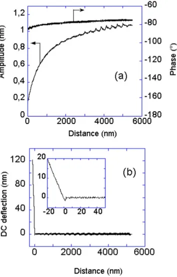
Figure6(a) shows the measured amplitude and phase of

the cantilever as the gap between the glass sphere and the glass substrate is reduced. Figure 6(b) presents the DC

deflection that allows one to determine the contact position of the two surfaces (zero distance) with accuracy better than 1 nm. From the measured amplitude and phase signals they use equations(21) and (22) to extract the interaction stiffness

and damping.

Figure7presents the damping coefficient1+g gH 0and

the stiffness kH versus the distance D. As the sphere approaches the glass surface, the damping coefficient increases due to the increase of the viscous drag force. However, the stiffness is unchanged and is equal to zero[63].

In the case of non-slip boundary conditions, the hydro-dynamic force that acts on the sphere is given by the Taylor equation, ph =  F R D z 6 23 H 2 ( )

where R is the sphere radius, D is the gap between the surfaces,η is the viscosity of the air and ż is the instantaneous velocity of the sphere. To take into account the boundary slip Vinogradova [62] introduced a correction function *f that depends on the distance D and the slip length b and showed that the expression of the viscous hydrodynamic force FHcan be written as: * g ph = =  F z f R D z 6 24 H H 2 ( ) if both surfaces have the same slip length b

⎜ ⎟ ⎜ ⎟ ⎡ ⎣⎢ ⎛ ⎝ ⎞⎠ ⎛⎝ ⎞⎠ ⎤ ⎦⎥ * = + + -f D b D b b D 2 6 1 6 ln 1 6 1 (25)

Figure 5.(a) Schematic illustration of a sphere vibrating close to a solid surface.(b) Amplitude and phase spectra of the cantilever obtained at two different positions from the glass surface(the dark lines are at D= 2000 μm and the gray lines are at D = 3 μm).

Figure 6.(a) The amplitude and phase of the cantilever measured as the glued sphere approaches the glass substrate. The oscillation frequency wasfixed at 139.8 kHz (20 Hz below the resonance frequency) and the oscillation amplitude far from the surface was 1.3 nm. The modulation on the amplitude signal is due to interferences due to multiple reflections on both surfaces (the cantilever and substrate) of the laser light used to measure the cantilever motion.(b) The DC deflection of the cantilever measured as the glued sphere approaches the glass surface, which allows one to determine the contact position of the two surfaces. The inset shows a zoom of the DC deflection curve at a small distance [63].

The inverse of the normalized hydrodynamic damping is given as * g g g ph = R D f 6 26 H 0 0 ₂ ( )

At large separation distanceDb, *f can be expanded in series at thefirst order

* »

-f b

D

1 2 (27)

so, at large separation distance, the hydrodynamic force is / g g g ph » + R D b 6 2 28 H 0 0 2( ) ( )

Figure8 presents the inverse of the normalized hydro-dynamic dampingγ0/γHobtained from the data presented in figure7. The linear extrapolation of the signal is represented by the dashed line. One can observe that the extrapolation curve does not pass through the origin, which indicates the presence of slip on the surfaces.

By fitting the data of the inverse of the normalized hydrodynamic damping using equation (26), Maali and

Bhushan [63] obtained a slip length of 118 ± 10 nm.

Fur-thermore, as shown in figure 8 the slip length b can be extracted in this experiment without any need to fit para-meters. The linear extrapolation of the inverse of the hydro-dynamic damping versus the distance intersects the distance axis at a position of 2b= 236 nm.

For the air at atmospheric pressure and ambient temp-erature, the mean free path is 67 nm according to Bird[8], and

thus, on the basis of the measured value of the slip length, the accommodation coefficient calculated using equation (1) is

aboutσ = 0.72.

Pan et al[64] have used the same techniques to measure

the slip length on different surfaces at standard pressure. The measurements show that the slip length does not depend on the oscillation amplitude of the cantilever. Their data show that on glass, graphite, and mica surfaces the slip length is 98 ± 19 nm, 234 ± 29 nm, and 110 ± 21 nm, respectively. The adsorbed water on the surfaces causes inelastic collision allowing a greater accommodation coefficient (smaller slip length). The wettability of graphite surfaces is lower than that of mica and glass surfaces, and it may explain the high slip length and low accommodation coefficient.

Siria et al[65], Honig et al [66], Honig and Ducker [67],

and Bowles and Ducker [68] have studied the thermally

dri-ven oscillation of a cantilever as it gradually approaches a wall. Under thermal excitation, the cantilever undergoes a vibration with amplitude that depends on the temperature and damping. In the approximation of a simple harmonic oscil-lator the power spectral density of the cantilever vibration is given by w w w w w w = - + PSD k T k Q D Q d 2 29 B 03 l 2 02 2 2 02 2 ( ) ( ) ( ) ( ) ( )

where kBis the Boltzmann constant, T is the temperature and Q(d) is the cantilever quality factor at distance d from the surface. The damping at distance d is obtained from the Figure 7.The normalized hydrodynamic damping 1+ γH/γ0and the

hydrodynamic interaction stiffness(kH) versus the gap (D) between

the sphere and the glass substrate. The inset shows 1+ γH/γ0versus

the distance on a semilogarithmic plot[63].

Figure 8.The inverse of the normalized hydrodynamic dampingγ0/

γHversus the distances between the sphere and the glass surface.

The solid line is thefit curve using theoretical expression

(equation (26)). The linear extrapolation of the signal is represented

by the dashed line and it intersects the distance axis at position 2b= 236 nm [63].

quality factor by g w = d k Q d 30 l 0 ( ) ( ) ( )

From an analysis of measurements of the damping versus the distance, Siria et al [65] reported perfect boundary slip

conditions for the airflow between a silicon cantilever and a flat cleaved optical fiber. Honig et al [67], Honig and Ducker

[66], and Bowles and Ducker [68] have used a similar

tech-nique(thermal excitation) and shown an opposite result. They measured afinite slip in agreement with the results of Maali and Bhushan[63], with a slip value ranging between 100 and

630 nm depending on the nature of the surfaces and their preparations.

Let us note that, in AFM experiments, the Knudsen number can be varied continuously over several decades by varying the distance between the two surfaces. As the dis-tance is reduced(increasing the Knudsen number) the canti-lever damping increases due to the viscousflow of confined gas between the surfaces. The measured damping is described by the continuous hydrodynamic approach that takes into account the slip of the gas on the surfaces.

6. Conclusion and outlook

We have described in this paper the most important techni-ques used to measure the slip length and the accommodation coefficient in a gas flow on isothermal surfaces. In all of the presented techniques, the gas slip is measured indirectly. The slip length related to the slip velocity is extracted from the measurement of the velocity of the drop(Millikan method), the deflection (rotating cylinder), the mass flow rate (mass flow rate experiment), and the force measurement (AFM experiment).

Particle image velocimetry, which was used successfully in the last decades to directly measure liquid slip close to solid surfaces [69, 70], was adopted to study gas flows. Some

preliminary works have recently focused on this technique within gas microchannels. However, thefirst attempts using either μPIV [54] or μMTV [55] have not been successfully

extended yet to the slipflow regime, and direct measurement of slip at the wall with these techniques is still challenging, particularly due to the strong diffusion effects encountered at the microscale[56].

Recent results of the Ducker group have shown that it is possible to modify the gas slip and the accommodation coefficients in situ [71]. By increasing the temperature of their

surface from 18°C to 40 °C, they showed that the slip increases from 290 nm to 500 nm. They explained the increase of the slip by the modification of the roughness of their surface, which opens the way to in situ control of gas flow on a given surface.

In this paper the surfaces are assumed isothermal; how-ever there are some situations where the temperature is not uniform. In such cases, the temperature gradient gives rise to the so-called thermal creep that induces a lateralflow velocity

of the gas. Understanding and optimization of this effect may open the way to the realization of gas micro-pumps controlled by temperature gradients.

References

[1] Maxwell J C 1879 On stresses in rarefied gases arising from inequalities of temperature Phil. Tran. R. Soc.170

231 56

[2] Millikan R A 1923 Coefficients of slip in gases and the law of reflection of molecules from the surfaces of solids and liquids Phys. Rev.21 217 38

[3] Meyer O E 1866 Pogg. Ann. 127 269

[4] Knudsen M 1909 Die Gesetze der Molekularströmung und der inneren Reibungsströmung der Gase durch Röhren Ann. d. Physik28 75

[5] Fisher W J 1909 The molecular and the frictional flow of gases in tubes Phys. Rev.29 325

[6] Morris D L, Hannon L and Garcia A L 1992 Slip length in a dilute gas Phys. Rev. A46 5279 81

[7] Veijola T, Kuisma H, Lahdenperä J and Ryhänen T 1995 Equivalent circuit model of the squeezed gasfilm in a silicon accelerometer Sens. Actuators, A Phys.48 239 48 [8] Bird G A 1998 Molecular Gas Dynamics and the Direct

Simulation of Gas Flows(Oxford: Clarendon Press) [9] Arkilic E B, Breuer K S and Schmidt M A 2001 Mass flow and

tangential momentum accommodation in silicon micromachined channels J. Fluid Mech.437 29 43 [10] Lockerby D A, Reese J M, Emerson D R and Barber R W 2004

Velocity boundary condition at solid walls in rarefied gas calculations Phys. Rev. E70 017303

[11] Cao B Y, Chen M and Guo Z Y 2005 Temperature dependence of the tangential momentum accommodation coefficient for gases Appl. Phys. Lett.86 091905

[12] Bao M and Yang H 2007 Squeeze film air damping in MEMS Sens. Actuators A Phys.136 3 27

[13] Cooper S M, Cruden B A, Meyyappan M, Raju R and Roy S 2004 Gas transport characteristics through a carbon nanotubule Nano Lett.4 377 81

[14] Bhushan B 2007 Springer Handbook of Nanotechnology 2nd edn(Heidelberg, Germany: Springer)

[15] Lauga E, Brenner M P and Stone H A 2007 Microfluidics: the no slip boundary condition Handbook of Experimental Fluid Dynamics ed C Tropea, A Yarin and J F Foss(New York: Springer)

[16] Maxwell J C 1867 On the dynamical theory of gases Phil. Trans. R. Soc.157 49 88

[17] Colin S 2005 Rarefaction and compressibility effects on steady and transient gasflows in microchannels Microfluid. Nanofluid.1 268 79

[18] Sharipov F 2011 Data on the velocity slip and temperature jump on a gas solid interface J. Phys. Chem. Ref. Data40

023101

[19] Millikan R A 1911 The isolation of an ion, a precision measurement of its charge, and the correction of Stokes’s law Phys. Rev.(Series I)32 349

[20] Millikan R A 1913 On the elementary electrical charge and the Avogadro constant Phys. Rev.2 109

[21] Millikan R A 1923 The general law of fall of a small spherical body through a gas, and its bearing upon the nature of molecular reflection from surfaces Phys. Rev.22 1

[22] Timiriazeff A 1913 ber die innere Reibung verdnnter Gase und ber den Zusammenhang der Gleitung und des

Temperatursprunges an der Grenze zwischen Metall und Gas Ann. Phys.345 971 91

[23] Stacy L J 1923 A determination by the constant deflection method of the value of the coefficient of slip for rough and for smooth surfaces in air Phys. Rev.21 239 49

[24] van Dyke K S 1923 The coefficients of viscosity and of slip of air and of carbon dioxide by the rotating cylinder method Phys. Rev.21 250 65

[25] Kuhlthau A R 1949 Air friction on rapidly moving surfaces J. Appl. Phys.20 217 23

[26] Comsa G, Fremerey J K, Lindenau B, Messer G and Rohl P 1980 Calibration of a spinning rotor gas friction gauge against a fundamental vacuum pressure standard J. Vac. Sci. Technol.17 642 4

[27] Gabis D S, Loyalka S K and Strovick T S 1996 Measurements of the tangential momentum accommodation coefficient in the transitionflow regime with a spinning rotor gauge J. Vac. Sci. Technol. A14 2592 8

[28] Tekasakul P, Bentz J A, Tompson R V and Loyalka S K 1996 The spinning rotor gauge: measurements of viscosity, velocity slip coefficients, and tangential momentum accommodation coefficients J. Vac. Sci. Technol. A14 2946 52

[29] Bentz J A, Tompson R V and Loyalka S K 1997 The spinning rotor gauge: measurements of viscosity, velocity slip coefficients, and tangential momentum accommodation coefficients for N2 and CH4 Vacuum48 817 24

[30] Bentz J A, Tompson R V and Loyalka S K 2001 Measurements of viscosity, velocity slip coefficients, and tangential momentum accommodation coefficients using a modified spinning rotor gauge J. Vac. Sci. Technol. A19 317 24 [31] Jousten K 2003 Is the effective accommodation coefficient of

the spinning rotor gauge temperature dependent? J. Vac. Sci. Technol. A21 318 24

[32] Gronych T, Ulman R, Peksa L and Repa P 2004 Measurements of the relative tangential momentum accommodation coefficient for different gases with a viscosity vacuum gauge Vacuum73 275 9

[33] McCulloh K E, Tilford C R, Ehrlich C D and Long F G 1987 Low rangeflowmeters for use with vacuum and leak standards J. Vac. Sci. Technol. A5 376 81

[34] Bergoglio M, Calcatelli A and Rumiano G 1995 Gas flowrate measurements for leak calibration Vacuum46 763 5 [35] Jousten K, Menzer H and Niepraschk R 2002 A new fully

automated gasflowmeter at the PTB for flow rates between 10 13 mol s−1and 10 6 mol s−1Metrologia39 519 29 [36] Pong K C, Ho C M, Liu J and Tai Y C 1994 Non linear

pressure distribution in uniform microchannels Application of Microfabrication to Fluid Mechanics ed

P R Bandyopadhyay, K S Breuer and C J Blechinger(New York: ASME) pp 51 6

[37] Harley J C, Huang Y, Bau H H and Zemel J N 1995 Gas flow in micro channels J. Fluid Mech.284 257 74

[38] Zohar Y, Lee S Y K, Lee W Y, Jiang L and Tong P 2002 Subsonic gasflow in a straight and uniform microchannel J. Fluid Mech.472 125 51

[39] Maurer J, Tabeling P, Joseph P and Willaime H 2003 Second order slip laws in microchannels for helium and nitrogen Phys. Fluids15 2613 21

[40] Colin S, Lalonde P and Caen R 2004 Validation of a second order slipflow model in rectangular microchannels Heat Transfer Eng.25 23 30

[41] Ewart T, Perrier P, Graur I and Méolans J G 2006 Mass flow rate measurements in gas microflows Exp. Fluids41 487 98 [42] Pitakarnnop J, Varoutis S, Valougeorgis D, Geoffroy S,

Baldas L and Colin S 2010 A novel experimental setup for gas microflows Microfluid. Nanofluid.8 57 72

[43] Bergoglio M, Mari D, Chen J, Si Hadj Mohand H, Colin S and Barrot C 2015 Experimental and computational study of gas flow delivered by a rectangular microchannels leak Measurement73 551 62

[44] Kandlikar S G, Garimella S, Li D, Colin S and King M R 2013 Heat Transfer and Fluid Flow in Minichannels and Microchannels 2nd edn(Oxford: Elsevier)

[45] Kandlikar S G, Colin S, Peles Y, Garimella S, Pease R F, Brandner J J and Tuckerman D B 2013 Heat transfer in microchannels 2012 status and research needs J. Heat Transf. Trans. ASME135 091001

[46] Aubert C and Colin S 2001 High order boundary conditions for gaseousflows in rectangular microchannels Microscale Thermophys. Eng.5 41 54

[47] Hsieh S S, Tsai H H, Lin C Y, Huang C F and Chien C M 2004 Gasflow in a long microchannel Int. J. Heat Mass Transf.47 3877 87

[48] Ewart T, Perrier P, Graur I and Méolans J G 2007 Tangential momemtum accommodation in microtube Microfluid. Nanofluid.3 689 95

[49] Ewart T, Perrier P, Graur I A and Méolans J G 2007 Mass flow rate measurements in a microchannel, from hydrodynamic to near free molecular regimes J. Fluid Mech.584 337 56 [50] Graur I, Perrier P, Ghozlani W and Meolans J 2009

Measurements of tangential momentum accommodation coefficient for various gases in plane microchannel Phys. Fluids21 102004

[51] Perrier P, Graur I A, Ewart T and Méolans J G 2011 Mass flow rate measurements in microtubes: from hydrodynamic to near free molecular regime Phys. Fluids23 042004 [52] Yamaguchi H, Hanawa T, Yamamoto O, Matsuda Y,

Egami Y and Niimi T 2011 Experimental measurement on tangential momentum accommodation coefficient in a single microtube Microfluid. Nanofluid.11 57 64

[53] Yamaguchi H, Matsuda Y and Niimi T 2012 Tangential momentum accommodation coefficient measurements for various materials and gas species J. Phys.: Conf. Series362

012035

[54] Yoon S Y, Ross J W, Mench M M and Sharp K V 2006 Gas phase particle image velocimetry(PIV) for application to the design of fuel cell reactantflow channels J. Power Sources

160 1017 25

[55] Samouda F, Colin S, Barrot C, Baldas L and Brandner J J 2015 Micro molecular tagging velocimetry for analysis of gas flows in mini and micro systems Microsyst. Technol.21 527 37

[56] Frezzotti A, Si Hadj Mohand H, Barrot C and Colin S 2015 Role of diffusion on molecular tagging velocimetry technique for rarefied gas flow analysis Microfluid. Nanofluid.19 1335 48

[57] Bonaccurso E, Kappl M and Butt H J 2002 Hydrodynamic force measurements: boundary slip of water on hydrophilic surfaces and electrokinetic effects Phys. Rev. Lett.88

076103

[58] Bonaccurso E, Butt H J and Craig V S J 2003 Surface roughness and hydrodynamic boundary slip of a newtonian fluid in a completely wetting system Phys. Rev. Lett.90 144501

[59] Neto C, Craig V S J and Williams D R M 2003 Evidence of shear dependent boundary slip in newtonian liquids Eur. Phys. J. E12 S71

[60] Neto C, Evans D R, Bonaccurso E, Butt H J and Craig V S J 2005 Boundary slip in newtonian liquids: a review of experimental studies Rep. Prog. Phys.68 2859

[61] Honig C D F and Ducker W A 2007 No slip hydrodynamic boundary condition for hydrophilic particles Phys. Rev. Lett.

98 028305

[62] Vinogradova O I 1995 Drainage of a thin liquid film confined between hydrophobic surfaces Langmuir11 2213

[63] Maali A and Bhushan B 2008 Slip length measurement of confined air flow using dynamic atomic force microscopy Phys. Rev. E78 027302

[64] Pan Y, Bhushan B and Maali A 2013 Slip length measurement of confined air flow on three smooth surfaces Langmuir29 4298 [65] Siria A, Drezet A, Marchi F, Comin F, Huant S and Chevrier J 2009 Viscous cavity damping of a microlever in a simple fluid Phys. Rev. Lett.102 254503

[66] Honig C D F and Ducker W A 2010 Effect of molecularly thin films on lubrication forces and accommodation coefficients in air J. Phys. Chem. C114 20114 9

[67] Honig C D F, Sader J E, Mulvaney P and Ducker W A 2010 Lubrication forces in air and accommodation coefficient measured by a thermal damping method using an atomic force microscope Phys. Rev. E81 056305

[68] Bowles A and Ducker W 2011 Gas flow near a smooth plate Phys. Rev. E83 056328

[69] Ou J and Rothstein J P 2005 Direct velocity measurements of theflow past drag reducing ultrahydrophobic surfaces Phys. Fluids17 103606

[70] Joseph P, Cottin Bizonne C, Benoît J M, Ybert C, Journet C, Tabeling P and Bocquet L 2006 Slippage of water past superhydrophobic carbon nanotube forests in microchannels Phys. Rev. Lett.97 156104

[71] Seo. D and Ducker W A 2013 In situ control of gas flow by modification of gas solid interactions PRL111 174502