A Comparative Study of Divisive and Agglomerative Hierarchical Clustering Algorithms

HAL Id: hal-02085844

https://hal.archives-ouvertes.fr/hal-02085844

Submitted on 31 Mar 2019

HAL is a multi-disciplinary open access archive for the deposit and dissemination of sci-entific research documents, whether they are pub-lished or not. The documents may come from teaching and research institutions in France or abroad, or from public or private research centers.

L’archive ouverte pluridisciplinaire HAL, est destinée au dépôt et à la diffusion de documents scientifiques de niveau recherche, publiés ou non, émanant des établissements d’enseignement et de recherche français ou étrangers, des laboratoires publics ou privés.

A Comparative Study of Divisive and Agglomerative

Hierarchical Clustering Algorithms

Maurice Roux

To cite this version:

Maurice Roux. A Comparative Study of Divisive and Agglomerative Hierarchical Clustering Algo-rithms. Journal of Classification, Springer Verlag, 2018, 35 (2), pp.345-366. �10.1007/s00357-018-9259-9�. �hal-02085844�

1 23

A Comparative Study of Divisive and

Agglomerative Hierarchical Clustering

Algorithms

1 23

Your article is protected by copyright and all

rights are held exclusively by Classification

Society of North America. This e-offprint is

for personal use only and shall not be

self-archived in electronic repositories. If you wish

to self-archive your article, please use the

accepted manuscript version for posting on

your own website. You may further deposit

the accepted manuscript version in any

repository, provided it is only made publicly

available 12 months after official publication

or later and provided acknowledgement is

given to the original source of publication

and a link is inserted to the published article

on Springer's website. The link must be

accompanied by the following text: "The final

publication is available at link.springer.com”.

___________________________________________

A Comparative Study of Divisive and

Agglomerative

Hierarchical Clustering Algorithms

Maurice Roux

Aix-Marseille Université, France

Abstract: A general scheme for divisive hierarchical clustering algorithms is

proposed. It is made of three main steps: first a splitting procedure for the subdivision of clusters into two subclusters, second a local evaluation of the bipartitions resulting from the tentative splits and, third, a formula for determining the node levels of the resulting dendrogram. A set of 12 such algorithms is presented and compared to their agglomerative counterpart (when available). These algorithms are evaluated using the Goodman-Kruskal correlation coefficient. As a global criterion it is an internal goodness-of-fit measure based on the set order induced by the hierarchy compared to the order associated with the given dissimilarities. Applied to a hundred random data tables and to three real life examples, these comparisons are in favor of methods which are based on unusual ratio-type formulas to evaluate the intermediate bipartitions, namely the Silhouette formula, the Dunn's formula and the Mollineda et al. formula. These formulas take into account both the within cluster and the between cluster mean dissimilarities. Their use in divisive algorithms performs very well and slightly better than in their agglomerative counterpart.

Keywords: Hierarchical clustering; Dissimilarity data; Splitting procedures;

Eval-uation of hierarchy; Dendrogram; Ultrametrics.

1. Introduction

Most papers using hierarchical clusterings employ one of the four popular agglomerative methods, namely the single linkage method, the average linkage method, the complete linkage method and Ward’s method. The goal of these methods is to represent the proximities, or the dissimilar-

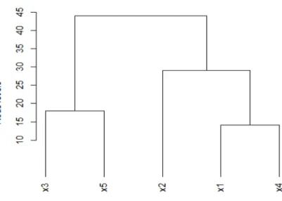
Figure 1. Dendrogram resulting from a hierarchical clustering program.

ities, between objects as a tree where the objects are situated at the end of the branches, generally at the bottom of the graph (Figure 1). The junctions of the branches are called the nodes of the tree; the node levels are supposed to represent the intensity of the ressemblance between the objects or clusters being joined.

In an agglomerative procedure (coined SAHN for Sequential

Agglomerative Hierarchical Non-overlapping by Sneath and Sokal,

1973), the tree is constructed bottom-up: at the beginning each

object x is considered as a cluster {x} called a singleton. Then each

step of the procedure consists in creating a new cluster by merging

the two closest clusters. This implies there is a way to compute the

dissimilarity or distance between two clusters. For instance, in the

usual average linkage method the distance between two clusters, C

and C

is the mean value of the between-cluster distances:

D(Cp , Cq ) = (1 / np nq)  { d(xi, xj) | xi  Cp , xj  Cq }, (1) where np and nq are the number of elements of Cp and Cq respectively, d(xi,

xj) is the given dissimilarity, or distance, between objects xi and xj .

The value of D(Cp, Cq) is then used as the node level for the junction of the branches issued from Cp and Cq . Indeed it can be shown that, this way, the usual procedures are monotonic. This means that if cluster C is included in a cluster C then their associated node levels LC and LC are in an increasing order:

C  C  LC  LC.

(2) This ensures that the hierarchical tree may be built without branch crossings. Thus, formula (1) is used first as a criterion for merging the clusters and, second, for determining the node levels of the hierarchy.

Divisive hierachical algorithms are built top-down: starting with the whole sample in a unique cluster they split this cluster into two subclusters which are, in turn, divided into subclusters and so on. At each step the two new clusters make up a so-called bipartition of the former. It is well known (Edwards and Cavalli-Sforza, 1965) that there are 2n - 1 _{– 1 ways of} splitting a set of n objects into two subsets. Therefore it is too time consuming to base a splitting protocol on the trial of all possible bipartitions. The present paper proposes to evaluate a restricted number of bipartitions to build up a working algorithm. Such an idea was developed a long time ago by Macnaughton-Smith et al. (1964) and reused by Kaufman and Rousseeuw (1990, Chap. 6, program DIANA).

With a view to applications in biology (genetics, ecology, …) all the algorithms proposed in this paper start with a distance, or dissimilarity matrix. The main objective of this study is to propose a general scheme for the elaboration of divisive hierarchical algorithms, where three main choices should apply at each step of the procedure:

i) a simplified way of splitting the clusters

ii) a formula to evaluate each of the considered bipartitions

iii) a formula to determine the node levels of the resulting hierarchy In this framework only complete binary hierarchies are looked for, so the choice of which cluster to split is not relevant: all clusters including two or more objects are split in turn, until there remains only singletons.

The above three points will be studied in the following (Sections 2, 3 and 4). Applying these principles gives rise to a family of algorithms described in Section 5. Then a practical benchtest is developed and used (Section 6) for comparing old and new algorithms. The main results are gathered (Section 6.4) and a concluding section terminates this paper (Section 7).

2. Splitting Procedures

A number of splitting procedures were designed in the past, the oldest one being by Williams and Lambert (1959). This procedure is said to be monothetic in the sense that object sets are split according to the values of only one variable. This idea was updated using one principal component instead of a single variable. It was first used by Reinert (1983) for qualitative variables and then by Boley (1998, Principal Directions Divisive Partitioning or PDDP, see Section 5.3). Another approach is set

up by using the k-means algorithm, with the parameter k = 2, to obtain a bipartition (Steinbach, Karypis, and Kumar, 2000). But, as this procedure uses vector data sets, and needs delicate initializations, it will not be studied in the present work.

Another approach to get around the complexity of splitting is to extract one, or several objects, from the set to be split. Macnaughton-Smith et al. (1964) proposed to select the most distant object from the cluster as a seed for a separate new cluster. Then they aggregate to this seed the objects which are closer to the new subset than to the rest of the current cluster. The distance used to evaluate the proximity between an object and a cluster is the mean value of the dissimilarities between this object and the objects in the cluster. A similar idea was developed by Hubert (1973): he suggested to use a pair of objects as seeds for the new bipartition. His choice was to select the two objects that are most dissimilar, and then to build up the two subclusters according to distances (or a function of distances, as the average value) to these seeds. Exploiting this idea Roux (1991, 1995) considered the bipartitions generated by all the pairs of objects, retaining the bipartition with the best evaluation of some a priori criterion. This procedure will be applied in the following.

The general scheme of the new algorithms is described in Table 1. The main operation is to manage the vector clus() which keeps the cluster numbers of the objects. These numbers decrease as the algorithm proceeds along the hierarchy. At the beginning, all objects belong to the same cluster numbered (2n – 1), where n is the number of objects under study. The first split gives raise to clusters numbered (2n – 2) and (2n – 3), except if one of them is a singleton; in such a case this singleton is considered as a node, the number of which is the current number of the object (between 1 and n) in the given dataset. These operations are pursued until all objects become singletons

3. Selection of Bipartitions

At each step of a usual agglomerative method the two candidate clusters Cp and Cq for a merging step may be considered as the bipartition {Cp , Cq} of the set Cp  Cq . For instance, in the case of the classical average link method, such a bipartition is evaluated by the mean value of the between-cluster distances.

In divisive methods, once the cluster Cp to be split is selected, the next step is to study a number of bipartitions {Cp , Cp } of Cp . Again the between-cluster average distances can be used for evaluating this split (Roux, 1991). However a number of criteria designed for the evaluation of any partition can be used. Thus both types of algorithms, divisive or agglomerative, rely upon a measure of similarity/dissimilarity between

Table 1. Outline of a divisive construction of a hierarchy. The splitting criterion splitcrit is supposed to be similar to a dissimilarity, thus the best partition is the one which maximize the criterion. P(C) designates the set of all pairs of elements of cluster C. Function B(p) assigns objects either to subset C’ or to subset C” of C according to their dissimilarity to i and j, the elements of pair p.

BASIC DIVISIVE CLUSTERING ALGORITHM

begin

input the n by n dissimilarity matrix dis

INITIALIZATIONS

for i := 1 to n do

clus(i) := 2*n – 1 w(2*n – 1) := n

end for

MAIN LOOP (h = node number)

for h := (2*n – 1) to (n + 1) step –1 do let C be a cluster with w(C) > 1

w(C) := cardinality(C) bestcrit := 0

SECONDARY LOOP (enumerates and evaluates bipartitions)

for each object pair p in P(C)

tempart := B(p)

currentcrit := splitcrit(tempart)

if currentcrit > bestcrit then

bestcrit := currentcrit bestpart := tempart

end if end for

CREATES OFFSPRINGS OF NODE h

C’ := first subset(bestpart) C” := second subset(bestpart)

diameter ≔ {dis(i, j)| i, j elements of C}

assign new numbers h’ and h” to clusters C’ and C”

update weights w(C’) and w(C”)

update vector clus for the elements of C output h, h’, h”, w(C), diameter

end for

sets. Such measures are described in this section which are then used as criteria in our algorithms. The list of these criteria is in Table 2 (Section 5). Whatever the adopted criterion, it should be noted that a series of very good bipartitions does not result automatically in a good hierarchy.

3.1 Five Distance-Like Formulas for Set Dissimilarities

In the following, Cp and Cp are tentative subsets of the current cluster Cp to be split.

Hierarchical Clustering Algorithms

The single linkage criterion is the lowest dissimilarity between objects of Cp and objects of Cp:

DSL(Cp , Cp) = Min { d(xi, xj) | xi  Cp, xj  Cp } . (3) The average linkage criterion is quite similar to formula (1):

DAV(Cp , Cp ) = (1 / |Cp|| Cp|) { d(xi, xj) | xi  Cp , xj  Cp } , (4) where |C| means the number of elements (cardinality) of C.

The complete linkage criterion is the largest dissimilarity between objects of Cp and objects of Cp ; in a divisive scheme this is not relevant since, for most bipartitions of Cp , the criterion has the same value, namely the diameter of Cp. Therefore, in a divisive framework, the formula is slighty modified as follows :

DCL (Cp , Cp ) = Max {  (Cp ),  (Cp )} , (5) where  (Cp ) and  (Cp ) are the diameters of Cp and Cp (respectively). It is clear that such formula defines a compactness measure. Therefore a good partition is reached for a low value of DCL .

Ward’s criterion may also be considered as a set dissimilarity criterion. Indeed, after the paper of Székely and Rizzo (2005), there exists an infinite family of algorithms similar to Ward’s. In the present study, the focus is only on two of them. One is the original algorithm as described by J.H. Ward (1963). The second is defined by the parameter  = 1 in the Székely-Rizzo family. Here the between-cluster dissimilarity involved by these algorithms are designated as DW1 (Ward’s original) and DW2 respectively, after Murtagh and Legendre (2014).

DW1(Cp , Cq ) = [ (2 / np nq)  { d2(xi, xj) | xi  Cp , xj  Cq } – (1 / n2p )  { d2(xi, xj) | xi  Cp , xj  Cp }

– (1 / n2q )  { d2(xi, xj) | xi  Cq , xj  Cq } ] (np nq / (np + nq)). (6) If the objects x are embedded in a vector space of real numbers, then this formula may be rewritten as:

DW1(Cp , Cq) = (np nq / (np + nq)) ∥g(xp) – g(xq)∥2 (7) where g(xp) and g(xq) are the centroids of clusters Cp and Cq, respectively. This formula shows that, in this case, DW1 is proportional to the between centroids squared distance.

DW2(Cp , Cq) = [ (2 / np nq)  { d(xi, xj) | xi  Cp , xj  Cq } – (1 / n2p )  { d(xi, xj) | xi  Cp , xj  Cp }

– (1 / n2

This second formula is very similar to the first one except for the exponent on the initial distances d(xi, xj). Székely and Rizzo (2005) put forward theoretical arguments to support formula (8), which should result in better partitions because, even with vector data, formula (8) cannot be rewritten in terms of between centroids distance as in formula (7). Thus it takes into account both the inter- and intra-cluster distances. The next section describes other ways to define set dissimilarities using intra- and inter-clusters relations.

3.2 Four Ratio-Type Criteria

The main idea for using such criteria is to take into account, not only the betwen cluster dissimilarities, but also the dissimilarities to the neighboring objects of the two clusters being studied. A popular, though dated, criterion is that of Dunn (1974), designed to evaluate a partition P with any number of elements:

Dunn (P) = Min{ Min { ( Cp , Cq ) | q  P, q  p }, p  P } /

Max { p | p  P }, (9)

where (Cp , Cq ) is the mean value of between-cluster dissimilarities (as formula (1)) and p is the diameter of subset Cp (i.e. the largest dissimilarity between objects included in Cp).

When evaluating the splitting of a cluster C into C and C the above formula reduces to:

DDu(C, C) =  (C, C) / Max{C , C}, (10) where C and Care the diameters of clusters C and C respect-ively.

But it is known that the diameter is rather sensitive to possible outliers; this is why the following variant is taken into account in the present study:

DDu(C, C) =  (C, C) / Max{( C C (C C)}, (11) where ( C C (resp. (C C) is the average value of within-cluster C (resp. C) dissimilarities. Indeed either formula (10) or formula (11) are of the type :

Between-cluster dispersion of dissimilarities / Within-cluster dispersion of dissimilarities

When one excessive dissimilarity value occurrs inside one cluster this may affect its diameter much more than the average value of within-cluster

dissimilarities. In addition, formula (11) looks more coherent with average values in both the numerator and the denominator of the ratio.

The Silhouette width (Rousseeuw, 1987; Kaufman and Rousseeuw, 1990) is considered in this study. For any object xi, included in a cluster C(xi), two functions, a and b, are defined and combined to get the Silhouette s(xi) of this object (|. | indicates the cardinality):

a(xi) = ( 1 / (|C(xi)| – 1)  { d(xi, xj) | xj  C(xi) } = ({xi}, C(xi) – {xi}), (12) b(xi) = Min{  ({xi}, Cp) | Cp  P – C(xi) }, (13) s(xi) = ( b(xi) – a(xi)) / Max { a(xi), b(xi) }. (14) The Silhouette width S(P) of a partition P is just the mean value of all the s(xi) for the xi covered by P

S(P) = (1 / n)  { s(xi) | xi   {Cp | p  P}}, (15) with n being the number of objects concerned by the current partition P. When C includes a bipartition {C , C} the formulas (12) and (13) become:

for xi in C a(xi) = ({xi}, C – {xi}) b(xi) = ({xi}, C), (16)

for xi in C a(xi) = ({xi}, C – {xi}) b(xi) = ({xi}, C), (16 bis) while the formal definitions of s(xi) and S(P) remain unchanged. A good partition for this criterion shows high values for parameters b’s, and low values for parameters a’s. Therefore a good partition is characterized by a high value of measure S.

Another ratio-type criteria was formulated by Mollineda et al. (2000) and used in an aggregative hierarchical algorithm. At each step of their algorithm, they define an isolation function  of two clusters taking into account the dissimilarities to other clusters under construction. In this formula i, j and k are clusters, and d is one of the usual between-cluster distances (average link, single link, etc …) :

 (i , j) =  { d(i, k) | k  K, k  j } / [ |K| - 2 ]. (17) In this formula, K is the set of all clusters available at the current step of the algorithm. It is worth noting that this formula is not symmetrical with respect to i and j, since (i , j) is not equal to (j , i). But they insert this function  in a relative dissimilarity D used to select the pair of clusters to be aggregated :

For this reason, they call their algorithm “relative hierarchical clustering” and we denote DRH this relative dissimilarity. Contrary to function , the relative dissimilarity DRH is symmetric with respect to i and j, and it could be used in either an agglomerative or a divisive scheme.

4. Determining the Node Levels

When used in an agglomerative scheme the usual five criteria examined in Section 3.1 are used without any problem for the represen-tation of the results: the criterion value becomes the level of the corresponding node, and the drawing of the hierarchical tree does not show any cross-over (or reversal) of the branches.

Unfortunately divisive procedures, in general, do not enjoy this property, because of the non-optimality of the successive splittings. A rule is then needed to obtain consistent node levels and a true tree representation. Kaufman and Rousseeuw (1990), in their program DIANA, use the diameter of the successive clusters as node levels. It is evident that the diameter of a subset C included in a set C is less than, or equal to, the diameter of C, fulfilling the monotonic condition (2). Thus the two subsets created by the splitting of C are always associated with lower (or equal) node levels.

Another way to settle consistent node levels would be to associate the ranks of the nodes according to the order in which they are created, starting with rank n – 1 for the top level, down to 1 for the last created node. But this method may not be satisfying; in effect, it may happen that a small homogeneous susbet would be separated at an early stage from the bulk of the objects. The corresponding node would then be associated with a high rank, in spite of its homogeneity. Another way to use ranks would be to renumber the nodes from the bottom up to the top, after completion of all the splittings, but this is not free of difficulties either.

Indeed the present discussion is of little use for the general purpose of comparing clustering algorithms, since the global evaluation of the results will be based on rank correlation methods (see Section 6.2). However, the users could be interested in getting coherent node levels, hence a working representation. In the present experiment, the node levels are determined, as in the program DIANA, by the diameters. For all divisive algorithms the node level is the diameter of the cluster being split. For agglomerative methods, the node level is the diameter of the new cluster formed at the aggregation step, except for those methods based on usual criteria, namely Single link, Average link, Complete link, Ward’s and Ward’s variant. In effect, these criteria fullfill the condition (2) when used in a aggregative framework allowing for a true hierarchical tree (without branch crossing).

5. New Algorithms Facing Old Ones

The nine formulas for set dissimilarities, described in section 3, may be used either for divisive or for agglomerative hierarchical algorithms. Following the suggestion of an anonymous reviewer both types of algorithms are studied with the same formulas. In divisive algorithms, according to the principles of Section 2, the between set dissimilarities are used to select one bipartition among those which are associated to a pair of elements; the bipartition resulting in the highest value of the criterion is retained for splitting the current cluster. In case of ties, the first split appearing is selected.

Due to the small modification adopted in the “Complete Link Divisive” method: the splitting criterion DCL (formula (4)), a compactness measure which should be minimized, is transformed into –DCL to enter the general framework of divisive algorithms which requires the maximization of the criterion.

In agglomerative algorithms, the same formulas are used to select the merging pairs of clusters. The pair which minimizes the criterion is merged in the current step. In case of ties, the first pair satisfying the criterion is adopted.

Thus, this part of the study leads to 18 computer programs, which are named after the formula they use in the list of Table 2. For the sake of comparisons, 3 other algorithms which do not follow the principles of Section 2, are included in the comparisons (Table 3). The first one is due to Macnaughton-Smith et al. (1964), whereas the last two are the Principal Direction Divisive Partitioning method (PDDP, Boley, 1998) and a variant of it. They are briefly described hereafter.

5.1 The Macnaughton-Smith et al. Algorithm

The method proposed by Macnaughton-Smith et al. could be con-sidered as a one-seed procedure. To split the cluster C, they choose as a seed the object x0 whose average distance to the other elements of C is maximum. The building of the bipartition begins with

C = C – {x0} and C = {x0}. (19) Next, for each object x in C, compute ({x}, C – {x}) and ({x}, C), and retain x1 as the one which maximizes

f(x) =  ({x}, C) – ({x}, C - {x}). (20) (has the same definition as above in formula (9)).Then the bipartition becomes

Table 2. List of the 9 criteria used in both divisive and agglomerative procedures. Note that the complete link criterion is modified when used in a divisive procedure (formula (5)).

Set dissimilarity criteria Formula no Types of criteria

Single link 3 Dist.

Average link divisive 4 Dist.

Complete link 5 Dist.

Ward’s original 6 Dist.

Ward’s Szekely-Rizzo 8 Dist.

Dunn’s original 10 Ratio

Dunn’s variant 11 Ratio

Silhouette 15 & 16 Ratio

Mollineda et al. 17 & 18 Ratio

Table 3. Supplementary divisive algorithms

Divisive methods Basic splitting principles

Macnaughton-Smith et al. Furthest object as initial seed + Transfer function

Principal Direction Divisive Partitionning (PDDP)

Coordinates on the first principal axis

PDDP variant As PDDP + Transfer function

C1 = C – {x1} and C1 = C  {x1}, (21)

and this process is continued until f(x) becomes negative. We call this process a one-way transfer function, since the only possible displacement is from the current cluster toward the new cluster being created.

5.2 The Principal Direction Divisive Partitioning Algorithm (PDDP) The PDDP method was first designed for the analysis of observations  variables data tables, but may be readily adapted by using the Principal Coordinates Analysis (PCoA, Gower, 1966). This technique is akin to the Principal components analysis (PCA) but applies to distance data. If the data are dissimilarities, they may not be euclidean, but the first principal direction is, in general, associated to a positive eigenvalue. In the PDDP algorithm, the first principal coordinate axis is used to create a dichotomy: those objects whose coordinates are negative are put into the first subset of the dichotomy, while the objects with positive, or null, coordinates make up the second subset. This PCoA is recomputed for each cluster with more than two objects, achieving a hierarchical divisive procedure.

Besides, in our study, a variant of this algorithm is used by the addition of a transfer function. After the main dichotomy using the first principal direction, a further step is taken which may move some objects (one at a time) from their actual assignment to the other one as long as they improve the inter-cluster mean dissimilarity. If C and Care the resulting subsets of the main dichotomy, then DAV(C,C) is calculated as the inter-cluster mean dissimilarity (formula (4)). Then for each object x, element of CrespCthis parameter is recomputed as DAV(C– {x}, Cx) (resp. DAV(C {x}, Cx)). Let x0 be the element which maximizes the value of this last computation among the elements of C  C if

DAV(C {x0}, Cx0) > DAV(C, C) when x0 belongs to C(22) DAV(C {x0}, Cx0) > DAV(C, C) when x0 belongs to C(22 bis) then x0 is moved from Cto C (resp. from Cto C). This procedure is continued until there is no more x satisfying inequality (22) or (22 bis). It may be called a two-way transfer function as the objects may be moved from any one of the two cluster under construction to the other.

With these 3 supplementary divisive algorithms it is a total of 21 algorithms which enter the following comparisons.

6. Practical Tests

The comparison of the above 12 divisive algorithms and 9 agglomerative ones is mainly dedicated to the quality of the results as measured by the goodness-of-fit of the results to the data. First the benchmark made of random datasets is described, followed by the treatement of some real life datasets. Next some thoughts about the goodness-of-fit criteria are developed. Then a tentative estimation of the algorithmic complexity is studied and, finally, a summary of the comparisons is set up.

6.1 Random Data Sets

A sample of 100 random datasets is set up. Each dataset is a matrix of 40 observations by 10 variables. All variables are generated from a uniform distribution over [0, 1]. All 10 variables are generated independently according to the same distribution. For each matrix the usual Euclidean distance is applied and treated by each of the algorithms. Although these data are far from real life data, they constitute a harsh benchmark and allow for a real competition among the programs.

The number of 40 observations per dataset is chosen as a common size when the objective is to build up a complete hierarchy (e.g. the

Pottery or the Leukemia examples, respectively 45 and 38 observations, in the next section). The computer programs may easily deal with 100 or 150 observations (e.g. Iris example with 150 observations), but the use and interpretation of the resulting hierarchies beyond this number of objects is rather difficult.

6.2 Real Life Datasets 6.2.1 Leukemia Dataset

Initially the data collected by Golub et al. (1999) were the expressions of more than 7000 genes in presence of 38 bone marrow samples from acute leukemia patients. By several preliminary treatments, the variables reduced to a homogeneous set of 100 genes. In addition these expressions were log-transformed before the computation of euclidean distances on the samples as suggested by Handl, Knowles, and Kell (2005) who used these data.

6.2.2 Pottery Dataset

The chemical composition of Romano-British pottery, obtained by Tubb, Parker, and Nickless (1980), gave rise to a data table of 45 samples and 9 quantitative variables (3 samples suspected to be erroneous were eliminated from the 48 initial observations). The data were first standardized prior to the computation of the usual euclidean distances between the samples.

6.2.3 Fisher’s Iris

The well known Fisher’s iris dataset is made of 150 samples including three species of irises, 50 samples per species (Fisher, 1936). There are four morphological variables, namely Sepal Length, Sepal Width, Petal Length, Petal Width. After global standardization the usual euclidean distances between samples are computed, and introduced as input in the clustering programs.

6.3 A Goodness-of-Fit Criterion

The most popular criterion to evaluate the results of hierarchical clusterings is certainly the Co-phenetic Correlation Coefficient (CPCC, Sokal and Rohlf, 1962). It needs the construction of the ultrametric distances associated with the dendrogram; then the CPCC is just the usual correlation coefficient between the input distances and the ultrametric distances, the values of which are laid out in two long vectors. Another

type of correlation coefficient, namely the Kendall’s tau, was used for evaluation of hierarchical algorithms by Cunningham and Ogilvie (1972).

In the present work the focus is rather oriented toward rank correlation methods. Indeed, when the user examines the hierarchy issued from the data, the user focuses mainly on the groups, and subgroups, disclosed by the algorithm; in other words the interest is mostly on the structure, or topology, of the tree rather than on the exact values of the within / between group distances. In addition, the results of some hierarchical algorithms are not given in terms of distances; this is the case in particular with the original Ward’s method, where the node levels represent variations of variance.

Kendall’s tau (Kendall, 1938) and Goodman-Kruskal‘s coefficient (Goodman and Kruskal, 1954) are both based on the ranks of the values being compared. Let d(xi, xj) be the input distance between objects xi and

xj, and u(xi, xj) the ultrametric distance between the same objects, resulting from a clustering algorithm (u(xi, xj) is the level to which objects xi and xj are linked in the dendrogram). The S+ _{index is the number of concordant} pairs of distances, and S– _{is the number of discordant pairs ; two pairs of} objects (xi, xj) and (xk, xl) constitute a “quadruple”, they are said to be concordant if:

d(xi, xj) < d(xk, xl ) and u(xi, xj) < u(xk, xl ), (23) they are said to be discordant if:

d(xi, xj) < d(xk, xl ) and u(xi, xj) > u(xk, xl ). (24) Then the Goodman coefficient is:

GK = (S+ _{– S}–_{) / (S}+ _{+ S}–_{), (25)} while the Kendall coefficient is:

  = (S+ _{– S}–_{) / (N (N – 1)/2), (26)}

where N is the number of distance pairs, that is (n (n – 1)/2) with n equal to the number of objects. These two coefficients differ by their denominator. Goodman-Kruskal denominator is the number of quadruples really taken into account (ties are not considered), while Kendall’s denominator is equal to the number of all quadruples, including the possible ties. It seems not reasonable to take into account the tied pairs which may be numerous due to the common level objects pairs dissimilarity, associated to the hierarchy.

In addition, the number of pairs really comparable may be much lower than in the case of a true correlation coefficient. For instance, in the

Table 4. Examples of numbers of inequalities in the computation of the Goodman-Kruskal coefficient in the Leukemia dataset. Agglo.Av.Link = Agglomerative Average Link method; Divisive M-S = Divisive Macnaughton-Smith et al. method. Total = total number

of quadruples with 38 objects; S+ _{= number of concordant quadruples (23); S}- _{= number of}

discordant quadruples (24); NC = number of quadruples with non comparable pairs; Ties = number of quadruples with equal hierarchical level pairs. The mean values (last two columns) are computed over the 21 numbers relative to the 21 algorithms studied.

Agglo.Av.Link Divisive M-S Mean values

# quadr. % total # quadr. % total # quadr. % total

Total 246753 246753 246753 S+ 143986 58.35 119390 48.38 130451.2 52.87 S- 35375 14.34 19645 7.96 41432.52 16.79 NC 19652 7.96 14626 5.93 18811.00 7.62 Ties 47740 19.35 93092 37.73 56058.24 22.72 G-K 0.6055 0.7174 0.514598

dendrogram of Figure 1, pairs (x1, x2) and (x1, x4) may be compared : (x1,

x4) < (x2, x4) because the cluster including x1 and x4 is itself included in the cluster including both x2 and x4. On the other hand (x1, x2) cannot be compared to (x2, x4) because both pairs are included in the same set {x1, x2, x4}. Again, no relation could be established between pairs (x1, x2) and (x3,

x5) for the same reason. These remarks make the computation of Goodman-Kruskal coefficient more complicated than applying a correlation coefficient between two dissimilarity matrices. In short a number of quadruples cannot be taken into account either because of equality of the associated node levels or because the two pairs of the quadruple, being in two separated branches, are not comparable.

To illustrate how much of these quadruples are discarded here are the numbers corresponding to the Leukemia dataset and for two clustering algorithms (Table 4). These two algorithms were taken as examples, they happen to be among the best ones as shown by their G-K index compared to the mean value reported in the last cell of this table.

6.4 Computing Considerations

The initial dissimilarity matrix must be preserved in the computer memory to allow for the repeated computations of non-standard between cluster dissimilarities. Each step of the divisive process needs the examination of objects pairs as potential seeds for the dichotomy. Since there is no updating formula like in agglomerative algorithms, selecting

one dichotomy implies to recompute the splitting criterion for each tentative bipartition. Then this evaluation is of order n2_{. The number of} bipartitions is also O(n2_{), therefore the complexity of one divisive step is}

O(n4_{). As the construction of the full binary hierarchy needs n – 1 steps,} the overall complexity of the proposed divisive algorithms is O(n5_{). This} involves a heavy computer task but is still possible for the moderate size of the target data.

All computations are programmed within the R-software. Computing times are given as indicative values since no effort has been done to optimize the program code. The scalability limitation comes from the dissimilarity matrix the size of which grows as n2 . But the main difficulty with big datasets is for the user to apprehend the resulting dendrogram.

6.5 Results and Discussion 6.5.1 Random Datasets

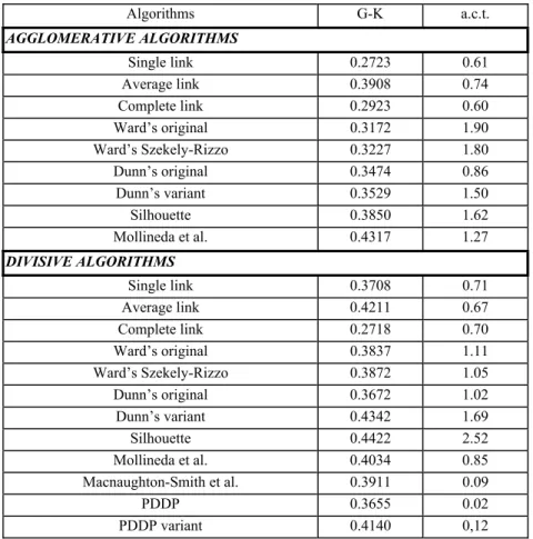
The experiment, conducted according to the above conditions, results in a table of 100 rows (random datasets) by 21 columns (algorithms : 9 agglomerative and 12 divisive methods). Each dataset, made of 40 observations, generates a 40  40 distance matrix. Any cell of the resulting table includes the Goodman-Kruskal coefficient relative to one data set and one algorithm. The higher the coefficient the better is the corresponding algorithm, since this coefficient is akin to a correlation coefficient.

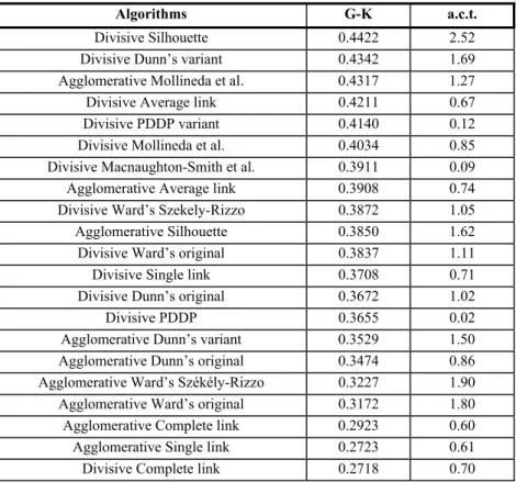
Table 5 gathers the average values of these coefficients over the 100 datasets, together with the corresponding average computing times. In Table 6, the algorithms are sorted by the average values of the Goodman-Kruskal coefficient in decreasing order. The best first two algorithms appear to be the Divisive Silhouette and the Divisive Dunn variant methods. Next come the Agglomerative method based on the Mollineda et al. formula, the Principal direction divisive method (with variant) and the Divisive average link method. Among these best first five algorithms only one follows an agglomerative scheme (based on Mollineda et al. formula) and their basic formulas are of the ratio type, except for the PDDP variant algorithm.

In the lower part of this ranking appear three algorithms, namely those which are the Agglomerative single link, Agglomerative complete link and the Divisive complete link. On average these three algorithms perform less well than the usual Agglomerative average link method.

Table 5. Average values of the Goodman-Kruskal coefficient (G-K) over 100 random data sets. a.c.t = average computing time, in seconds.

Algorithms G-K a.c.t. AGGLOMERATIVE ALGORITHMS Single link 0.2723 0.61 Average link 0.3908 0.74 Complete link 0.2923 0.60 Ward’s original 0.3172 1.90 Ward’s Szekely-Rizzo 0.3227 1.80 Dunn’s original 0.3474 0.86 Dunn’s variant 0.3529 1.50 Silhouette 0.3850 1.62 Mollineda et al. 0.4317 1.27 DIVISIVE ALGORITHMS Single link 0.3708 0.71 Average link 0.4211 0.67 Complete link 0.2718 0.70 Ward’s original 0.3837 1.11 Ward’s Szekely-Rizzo 0.3872 1.05 Dunn’s original 0.3672 1.02 Dunn’s variant 0.4342 1.69 Silhouette 0.4422 2.52 Mollineda et al. 0.4034 0.85 Macnaughton-Smith et al. 0.3911 0.09 PDDP 0.3655 0.02 PDDP variant 0.4140 0,12

6.5.2 Real life Datasets

Table 7 contains the evaluations of the 21 algorithms for the three real life examples described in section 6.2.

Focusing on the best five algorithms leads to mainly select divisive algorithms except for the Pottery example where it is found the Agglomerative version of Mollineda et al. formula (first rank) and the usual Agglomerative average link algorithm (4-th rank) performs the best. A good set of evaluations is obtained for the Macnaughton-Smith et al. divisive method.

Table 6. Average values of the Goodman-Kruskal coefficient (G-K) over 100 random data sets, sorted in decreasing order. a.c.t. = average computing time.

Algorithms G-K a.c.t.

Divisive Silhouette 0.4422 2.52

Divisive Dunn’s variant 0.4342 1.69

Agglomerative Mollineda et al. 0.4317 1.27

Divisive Average link 0.4211 0.67

Divisive PDDP variant 0.4140 0.12

Divisive Mollineda et al. 0.4034 0.85

Divisive Macnaughton-Smith et al. 0.3911 0.09

Agglomerative Average link 0.3908 0.74

Divisive Ward’s Szekely-Rizzo 0.3872 1.05

Agglomerative Silhouette 0.3850 1.62

Divisive Ward’s original 0.3837 1.11

Divisive Single link 0.3708 0.71

Divisive Dunn’s original 0.3672 1.02

Divisive PDDP 0.3655 0.02

Agglomerative Dunn’s variant 0.3529 1.50

Agglomerative Dunn’s original 0.3474 0.86

Agglomerative Ward’s Székély-Rizzo 0.3227 1.90

Agglomerative Ward’s original 0.3172 1.80

Agglomerative Complete link 0.2923 0.60

Agglomerative Single link 0.2723 0.61

Divisive Complete link 0.2718 0.70

6.5.3 Discussion

Either with artificial datasets or with real life datasets, the Divisive algorithm based on the Silhouette formula performs very well. In addition, according to the Goodman-Kruskal coefficient, there is a clear trend for the divisive algorithms to be superior to their agglomerative counterpart. But none of them can be definitely declared as the best algorithm. Indeed almost all algorithms may, in turn, show the best value of this quality coefficient, depending on the data at hand.

Another interesting result of this study is that the ratio type formulas (Silhouette, Dunn’s, Mollineda’s and their variants), which take into account the local environment of the clusters, provide with better results than the classical distance like formulas.

Table 7. Values of the Goodman-Kruskal coefficient (G-K) for three real life datasets. c.t. = computing time in seconds. The best values are in bold italic characters.

Algorithms Pottery (45 obs.) Leukemia (38 obs.) Iris (150 obs.)

G-K c.t. G-K c.t. G-K c.t. AGGLOMERATIVE ALGORITHMS Single link 0.8009 0.91 0.4447 0.48 0.7725 132.58 Average link 0.8056 1.13 0.6055 0.66 0.8448 140.34 Complete link 0.8042 0.91 0.2928 0.5 0.7025 133.35 Ward’s original 0.7906 2.69 0.4473 1.55 0.8225 200.26 Ward’s Szekely-Rizzo 0.6819 2.57 0.4372 1.46 0.8262 195.14 Dunn’s original 0.6836 1.27 0.3891 0.72 0.7653 148.93 Dunn’s variant 0.7916 2.01 0.4297 0.94 0.8384 184.3 Silhouette 0.8048 2.43 0.6444 1.39 0.8324 199.2 Mollineda et al. 0.8066 1.85 0.6225 1.08 0.8460 180.14 DIVISIVE ALGORITHMS Single link 0.8063 0.71 0.6048 0.61 0.8186 66.08 Average link 0.8039 0.76 0.5269 0.84 0.7900 63.84 Complete link 0.6419 1.22 0.3018 0.75 0.4084 141.64 Ward’s original 0.7934 1.72 0.4425 1.01 0.8503 70.23 Ward’s Szekely-Rizzo 0.6851 1.54 0.4425 0.96 0.8483 66.13 Dunn’s original 0.8048 1.25 0.5753 0.78 0.8469 112.26 Dunn’s variant 0.7825 1.79 0.6909 1.81 0.8434 109.26 Silhouette 0.8056 2.62 0.6007 2.25 0.8545 255.27 Mollineda et al. 0.6896 1.04 0.5532 1.14 0.7159 99.81 Macnaughton-Smith et al. 0.8054 0.13 0.7174 0.09 0.8512 1.51 PDDP 0.5013 0.1 0.3477 0.15 0.8238 0.16 PDDP variant 0.6853 0.13 0.5195 0.16 0.8511 1.24

However, the usual Agglomerative Average Link method reaches a rather medium average value for the Goodman-Kruskal coefficient (G-K = 0.3908 at the 8-th rank out of 21) with random datasets, but it resulted in a very good value with Pottery example (4-th rank with G-K = 0.8056, the best value being 0.8066 for the Agglomerative Mollineda‘s algorithm). A similar observation can be made for the Macnaughton-Smith et al. divisive method: at the 7-th rank in the random datasets (G-K = 0.3911) and ranks 5, 1 and 2 in the Pottery, Leukemia and Iris datasets respectively.

As expected the highest computing times are reached for divisive algorithms and for those algorithms based on ratio formulas, especially the Silhouette formula which is rather complicated.

7. Conclusion

The present work aims at the treatment of moderate size datasets (forty objects in the random examples), but with a search for the quality of the results. It focuses on distance or dissimilarity data and it studies the methods to obtain complete binary hierarchies. The formulas to evaluate the quality of a bipartition may be used either in an agglomerative algorithm or in a divisive one. The popular formulas used in pairwise aggregative procedures, namely the single linkagr, the complete linkage and the average linkage methods and two versions of Ward’s algorithm are retained. While other four formulas are based on criteria involving a ratio of between-group dissimilarities and within-group dissimilarities.

Thus, this study compared a set of 9 agglomerative and 9 divisive clustering algorithms which are built with the above formulas. Another set of 3 divisive hierarchical clustering algorithms are added leading to a total of 21 algorithms. The divisive algorithms are intended as competitors of the classical agglomerative algorithms.

An important argument of the present work is that it is possible to separate the computation of the hierarchical node levels from the criterion used for splitting a cluster. The question of a readable dendrogram (without crossing branches over) is then solved by using the diameters of the clusters.

This does not hamper the internal evaluation of the results, that is to say the comparison of the hierarchy with the initial data, thanks to the Goodman-Kruskal correlation coefficient. Comparing the order relation induced by the successive inclusions of the clusters with the order relation associated with the input dissimilarities, this correlation coefficient provides with an evaluation independent of the node levels, and concentrates on the shape, or topology, of the resulting dendrogram which is certainly the main interest of the user.

Applied to a sample of a hundred random datasets these principles allow for a ranking of the algorithms. The best ones are based on ratio-type splitting criteria: the Silhouette formula and a variant of Dunn’s formula for partitions. At the lower end of this ranking appear three procedures : Divisive complete link, together with the Agglomerative complete link and single link based procedures, which dissuades to use them.

In three real life examples the divisive algorithms based on Silhouette and Dunn’s formula are present in the “top five” best algor-ithms. In these examples the other divisive algorithms based on ratio type formulas, appear in the best five results.

Further works, for divisive algorithms, could be considered in two directions; the first direction would be the treatment of bigger data sets, the second one would be the combination of two (or more) of the studied

algorithms. Dealing with big datasets needs to establish some stopping rules to avoid the complexity of a complete binary hierarchy, and a supplementary step to select the clusters to be split. It may also require the evaluation of a restricted number of bipartitions in order to limit the computing load.

References

BOLEY, D. (1998), “Principal Directions Divisive Partitioning”, Data Mining and

Knowledge Discovery, 2(4), 325–344.

CUNNINGHAM, K.M., and OGILVIE, J.C. (1972), “Evaluation Of Hierarchical Grouping

Techniques : A Preliminary Study”, Computer Journal, 15(3), 209–213.

DUNN, J.C. (1974), “Well Separated Clusters and Optimal Fuzzy Partitions”, Journal of

Cybernetics, 4, 95–104.

EDWARDS, A.W.F., and CAVALLI-SFORZA, L.L. (1965), “A Method for Cluster

Analysis”, Biometrics, 21(2), 362–375.

FISHER, R. A. (1936), “The Use of Multiple Measurements in Taxonomic Problems”,

Annals of Eugenics, 7, 179–188.

GOLUB, T.R., SLONIM, D.K., TAMAYO, P., HUARD, C., GAASENBEEK, M., MESIROV, J.P., COLLER, H., LOH, M.L., DOWNING, J.R., CALIGIURI, M.A.,

BLOOMFIELD, C.D., and LANDER, E.S. (1999), “Molecular Classification of

Cancer: Class Discovery Monitoring and Class Prediction by Gene Expression

Monitoring”, Science, 286, 531–537.

GOODMAN, L., and KRUSKAL, W. (1954), “Measures of Association for

Cross-Validations, Part 1”, Journal of the American Statistical Association, 49, 732–764.

GOWER, J.C. (1966), “Some Distance Properties of Latent Root and Vector Methods Used

in Multivariate Analysis”, Biometrika, 53(3,4), 325–338.

HANDL, J., KNOWLES, J., and KELL, D.B. (2005), “Computational Cluster Validation in

Post-Genomic Data Analysis”, Bioinformatics, 21(15), 3201–3212.

HUBERT, L.(1973), “Monotone Invariant Clustering Procedures”, Psychometrika, 38(1),

47–62.

KAUFMAN L., and ROUSSEEUW, P.J. (1990), Finding Groups in Data, New York: Wiley.

KENDALL, M.G. (1938), “A New Measure of Rank Correlation”, Biometrika. 30(1-2),

81–93.

MACNAUGHTON-SMITH, P., WILLIAMS, W.T., DALE, M.B., and MOCKETT L.G.

(1964), “Dissimilarity Analysis: A New Technique of Hierarchical Sub-Division”,

Nature, 202, 1034–1035.

MOLLINEDA, R.A., and VIDAL, E. (2000), “A Relative Approach to Hierarchical

Clustering”, in Pattern Recognition and Applications, eds. M.I. Torres and A.

Sanfeliu, Amsterdam : IOS Press, pp 19–28.

MURTAGH, F., and LEGENDRE P. (2014), “Ward’s Hierarchical Agglomerative Method

: Which Algorithms Implement Ward’s Criterion? ” Journal of Classification, 31,

274–295.

REINERT, M. (1983),

“

Application à l'Analyse Lexicale par Contexte

”

ROUSSEEUW, P.J. (1987), “Silhouettes: A Graphical Aid to the Interpretation and

Validation of Cluster Analysis”, Journal of Computational and Applied Mathematics,

20, 53–65.

ROUX, M. (1991), “Basic Procedures in Hierarchical Cluster Analysis”, in Applied

Multivariate Analysis in SA–R and Environmental Studies, eds. J. Devillers and W.

Karcher, Dordrecht : Kluwer Academic Publishers, pp 115–135.

ROUX, M. (1995),“About Divisive Methods in Hierarchical Clustering”, in Data Science

and Its Applications, eds. Y. Escoufier, C. Hayashi, B. Fichet, N. Ohsumi, E. Diday,

Y. Baba, and L. Lebart, Tokyo: Acadademic Press, pp 101–106.

SNEATH, P.H.A., and SOKAL, R.R. (1973), Numerical Taxonomy, San Francisco: W.H. Freeman and Co.

SOKAL, R.R., and ROHLF, F.J. (1962),

“

Methods

”

STEINBACH, M., KARYPIS, G., and KUMAR, V. (2000),

“

Clustering Techniques

”

Minneapolis, USA.

SZÉKELY, G.J., and RIZZO, M.L. (2005),

“

Between-Within Distances: Extending Ward's Minimum Variance Method

”

Classification, 22, 151–183.

TUBB, A., PARKER, N.J., and NICKLESS, G. (1980), “The Analysis of Romano-British

Pottery by Atomic Absorption Spectrophotometry”, Archaeometry, 22, 153–171.

WARD, J.H. JR. (1963),

“

”

Journal of the American Statisitcal Association, 58, 236–244.

WILLIAMS, W.T., and LAMBERT, J.M. (1959),

“