Towards high precision internal camera calibration

(1)

HAL Id: tel-01133601

https://pastel.archives-ouvertes.fr/tel-01133601

Submitted on 19 Mar 2015

HAL is a multi-disciplinary open access archive for the deposit and dissemination of sci-entific research documents, whether they are pub-lished or not. The documents may come from teaching and research institutions in France or abroad, or from public or private research centers.

L’archive ouverte pluridisciplinaire HAL, est destinée au dépôt et à la diffusion de documents scientifiques de niveau recherche, publiés ou non, émanant des établissements d’enseignement et de recherche français ou étrangers, des laboratoires publics ou privés.

Victoria Rudakova

To cite this version:

Victoria Rudakova. Towards high precision internal camera calibration. Signal and Image Processing. Université Paris-Est, 2014. English. �NNT : 2014PEST1039�. �tel-01133601�

(2)

École Doctorale Paris-Est

Mathématiques & Sciences et Technologies de l’Information et de la Communication

Thèse de doctorat

de l’UNIVERSITÉ PARIS EST

Domaine : Informatique

présentée par Victoria Rudakova pour obtenir le grade de

Docteur de l’UNIVERSITÉ PARIS EST

Vers l’étalonnage interne de caméra à haute précision

Soutenue publiquement le XXI janvier 2014 devant le jury composé de :

Rapporteurs : _{Andrès Almansa} - Telecom ParisTech

David Fofi - Université de Bourgogne

Directeur : _{Pascal Monasse} - École des Ponts ParisTech

Examinateurs : _{Marc Pierrot-Deseilligny - ENSG Paris-Est}

(3)

6, Av Blaise Pascal - Cité Descartes Champs-sur-Marne

77455 Marne-la-Vallée cedex 2 France

Université Paris-Est Marne-la-Vallée École Doctorale Paris-Est MSTIC Département Études Doctorales 6, Av Blaise Pascal - Cité Descartes Champs-sur-Marne

(4)

École Doctorale Paris-Est

Mathématiques & Sciences et Technologies de l’Information et de la Communication

PHD thesis

of UNIVERSITÉ PARIS EST

Speciality : Informatics

presented by Victoria Rudakova to obtain the title of

PhD of Science of UNIVERSITÉ PARIS EST

Towards high precision internal camera calibration

Presented on XXI january 2014 before the jury composed of :

Reviewers : _{Andrès Almansa} - Telecom ParisTech

David Fofi - Université de Bourgogne

Advisor : _{Pascal Monasse} - École des Ponts ParisTech

Examinators : _{Marc Pierrot-Deseilligny - ENSG Paris-Est}

(5)

6, Av Blaise Pascal - Cité Descartes Champs-sur-Marne

Université Paris-Est Marne-la-Vallée École Doctorale Paris-Est MSTIC Département Études Doctorales 6, Av Blaise Pascal - Cité Descartes Champs-sur-Marne

(6)

Acknowledgements

The thesis was conducted at Ecole des Ponts Paris-TECH, and was funded by the Agence Nationale de la Recherche, Callisto project (ANR-09-CORD-003). I would like to thank ANR for giving me such an opportunity to come and do my studies in France.

I am very grateful to Pascal Monasse who supervised me during these three years, for his explanations, patience and availability. His remarkable scientific and personal qualities helped me a lot in understanding, analysing, and solving the encountered problems during my thesis. I appreciate and feel very grateful for this. Also, I was happy to belong to the IMAGINE lab during last years and enjoyed occurred interactions - whether scientific or not.

I also appreciate the jury members of the thesis: Andrès Almansa, David Fofi, Jean-Michel Morel and Marc Pierrot-Deseilligny. Thank you for being interested in my work, for your comments and questions.

For the constant support I thank my friends and family (in alphabetical order): Anna, Cécile, Natalia Lyubova, Olga, Q.J., Steve P., Yumiko; and I thank all my Parisian friends and people from club de Neuilly-sur-Marne for sharing great time in the city of lights and Ile-de-France region.

(7)

(8)

Titre Vers l’étalonnage interne de caméra à haute précision

Établissment École des Ponts ParisTech IMAGINE / CERTIS Nobel B006

6, Av Blaise Pascal - Cité Descartes, Champs-sur-Marne 77455 Marne-la-Vallée cedex 2 - France

Resumé Cette thèse se concentre sur le sujet de l’étalonnage interne de la caméra et, en particuler, sur les aspects de haute précision. On suit et examine deux fils principaux: la correction d’une aberration chromatique de lentille et l’estimation des paramétres intrinsèques de la caméra.

Pour la problème de l’aberration chromatique, on adopte une méthode de post-traitement numérique de l’image, afin de se débarrasser des artéfacts de couleur provoqués par le phénomène de dispersion du système d’objectif de la caméra, ce qui produit une désalignement perceptible des canaux couleur. Dans ce contexte, l’idée principale est de trouver un modéle de correction plus général pour réaligner les canaux de couleur que ce qui est couramment utilisé – différentes variantes du polynôme radial. Celui-ci peut ne pas être suffisamment général pour assurer la correction précise pour tous les types de caméras. En combinaison avec une détec-tion précise des points clés, la correcdétec-tion la plus précise de l’aberradétec-tion chromatique est obtenue en utilisant un modèle polynomial qui est capable de capter la nature physique du décalage des canaux couleur. Notre détection de points clés donne une précision allant jusqu’à 0,05 pixels, et nos expériences montrent sa grande résistance au bruit et au flou. Notre méthode de correction de l’aberration, par opposition aux logiciels existants, montre une erreur géométrique résiduelle inférieure à 0,1 pixels, ce qui est la limite de la perception de la vision humaine.

En ce qui concerne l’estimation des paramètres intrinsèques de la caméra, la question est de savoir comment éviter la compensation d’erreur résiduelle inhérente aux méthodes globales d’étalonnage, dont le principe fondamental consiste à estimer tous les paramètres de la caméra ensemble – l’ajustement de faisceaux. Détacher les estimations de la distorsion de la caméra et des paramètres intrinséques devient possible lorsque la distorsion est compensée séparément. Cela peut se faire au moyen de la harpe d’étalonnage, récemment développée, qui calcule le champ de distorsion en utilisant la mesure de la rectitude de fils tendus dans différentes orientations. Une autre difficulté, étant donnée une image déjà corrigée de la distorsion, est de savoir comment éliminer un biais perspectif. Ce biais dû à la perspective est présent quand on utilise les centres de cibles circulaires comme points clés, et il s’amplifie avec l’augmentation de l’angle de vue. Afin d’éviter la modélisation de chaque cercle par une fonction conique, nous intégrons plutôt une fonction de transformation affine conique dans la procédure de minimisation pour l’estimation de l’homographie.

(9)

Nos expériences montrent que l’élimination séparée de la distorsion et la correction du biais perspectif sont efficaces et plus stables pour l’estimation des paramètres intrinsèques de la caméra que la méthode d’étalonnage globale.

Mots clés Étalonnage interne, matrice de caméra, aberration chromatique latérale, étalonnage de haute précision, correction de la distorsion, biais perspectif, points de contrôle circulaires.

(10)

Title Towards high precision internal camera calibration

Institution École des Ponts ParisTech IMAGINE / CERTIS Nobel B006

6, Av Blaise Pascal - Cité Descartes, Champs-sur-Marne 77455 Marne-la-Vallée cedex 2 - France

Abstract This dissertation focuses on internal camera calibration and, especially, on its high-precision aspects. Two main threads are followed and examined: lens chromatic aberration correction and estimation of camera intrinsic parameters.

For the chromatic aberration problem, we follow a path of digital post-processing of the image in order to get rid of the color artifacts caused by dispersion phenomena of the camera lens system, leading to a noticeable color channels misalignment. In this context, the main idea is to search for a more general correction model to realign color channels than what is commonly used – different variations of radial polynomial. The latter may not be general enough to ensure stable correction for all types of cameras. Combined with an accurate detection of pattern keypoints, the most precise chromatic aberration correction is achieved by using a polynomial model, which is able to capture physical nature of color channels misalignment. Our keypoint detection yields an accuracy up to 0.05 pixels, and our experiments show its high resistance to noise and blur. Our aberration correction method, as opposed to existing software, demonstrates a final geometrical residual error of less than 0.1 pixels, which is at the limit of perception by human vision.

When referring to camera intrinsics calculation, the question is how to avoid residual error compensation which is inherent for global calibration methods, the main principle of which is to estimate all camera parameters simultaneously - the bundle adjustment. Detachment of the lens distortion from camera intrinsics be-comes possible when the former is compensated separately, in advance. This can be done by means of the recently developed calibration harp, which captures dis-tortion field by using the straightness measure of tightened strings in different ori-entations. Another difficulty, given a distortion-compensated calibration image, is how to eliminate a perspective bias. The perspective bias occurs when using cen-ters of circular targets as keypoints, and it gets more amplified with increase of view angle. In order to avoid modelling each circle by a conic function, we rather incorporate conic affine transformation function into the minimization procedure for homography estimation. Our experiments show that separate elimination of distortion and perspective bias is effective and more stable for camera’s intrinsics estimation than global calibration method.

Keywords Internal calibration, camera matrix, lateral chromatic aberration, high precision calibration, lens distortion correction, perspective bias, circular

(11)

(12)

Introduction - version française

Cette thèse se concentre sur les aspects de précision de l’étalonnage interne de l’appareil photo, et il appartient au projet de recherche CALLISTO (Calibration en vision stéréo par méthodes statistiques) financé par l’ANR (Agence Nationale de la Recherche), dont l’objectif final est la reconstruction des scènes 3D en haute précision. Pour la dissertation deux directions principales d’étalonnage ont été choisis: la correction de l’aberration chromatique et l’extraction de paramétres internes de camèra.

La raison principale pour laquelle nous nous référons à l’étalonnage de l’appareil photo dans le contexte de scènes 3D de haute précision parce qu’elle est la première étape dans une chaîne de reconstruction 3D, et si l’étalonnage n’est pas fait cor-rectement, il va ruiner les étapes suivantes, peu importe le degré de précision ils ont; l’erreur sera propagée, amplifiée ou mélangée avec les erreurs suivantes. En conséquence, cela conduira á un modèle 3D imprécis. Bien qu’il ne semble pas pos-sible d’améliorer directement la précision globale utilisant les données imprécises obtenus, la bonne façon est de se référer à chaque composante séparément et étud-ier sa précision. Par ailleurs, le calibrage de la caméra doit être fait une fois, jadis les réglages de l’appareil sont fixes.

Lorsqu’on référe au problème d’étalonnage, une question se pose - est-ce que le sujet peut être considéré complet et résolu, ou s’il y a toujours de travail qui peut être fait dans la domain. La question n’est pas simple et dépend de ce qui est con-sidéré comme une contribution à la recherche de valeur et aussi si la solution actuelle satisfait les résultats requis. Par exemple, les méthodes d’étalonnage et de modèles qui étaient valables pour les exigences de précision dernières, ne sont plus satisfais-ant pour les nouveaux appareils photo numériques avec une résolution plus élevée, ce qui signifie que le sujet n’est pas entièrement fermé. L’augmentation de résolu-tion du capteur concerne également le problème de l’aberrarésolu-tion chromatique. Des tests de perception visuelle ont été effectués afin de voir que les solutions existantes ne sont plus si efficaces.

1.1 Correction de l’aberration chromatique

La première partie de la thèse est consacrée à la méthode précise pour la correction de l’aberration chromatique. En raison de l’évolution plus rapide de la technologie des capteurs par rapport à la technologie optique pour les systèmes d’imagerie, la perte de qualité de résultat qui se produit en raison de l’aberration chromatique latérale est de plus en plus importantes pour l’augmentation de la résolution du

(15)

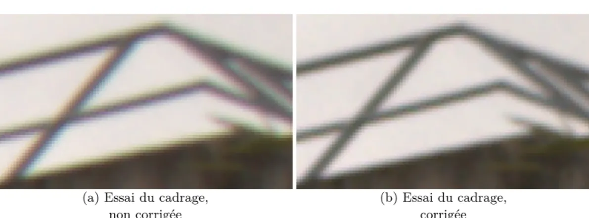
(a) Essai du cadrage, non corrigée

(b) Essai du cadrage, corrigée

Figure 1.1: Recadrée et agrandie dans l’image de la caméra Canon EOS 40D, avant (a) et après (b) la correction de l’aberration chromatique par notre méthode. Re-marquez les franges de couleurs atténuées au niveau des bords entre (a) et (b) des images.

capteur. Nous cherchons à trouver de nouvelles façons de surmonter les limites de qualité de l’image obtenue pour des raisons de performances et systèmes de lentilles plus légers.

La principale raison de l’aberration chromatique est le phénomène physique qui s’appelle réfraction. C’est la cause pour laquelle les canaux de couleur se concentrer un peu différemment. En raison de l’aberration, les couches de couleur sont légère-ment décalée lorsque l’image numérique est récupérée, ce qui conduit à des franges de couleur au niveau des zones de contraste élevés et les bords de l’image. Pour les applications de haute précision, lorsque l’utilisation d’informations de couleur devi-ent importante, il est nécessaire de corriger ces défauts avec précision. Figure 1.1 montre l’effet de notre correction de l’aberration chromatique sur une image réelle. D’une manière générale, l’aberration peut être classé en deux types: axiale et latérale. La première se produit lorsque différentes longueurs d’onde se concentrent à différentes distances de la lentille - en images numériques, il produit effet de flou depuis canaux bleu et rouge sont vaporisé (en supposant que le canal vert est au point). Un défaut latérale se produit lorsque les longueurs d’onde se concentrent sur differénts points du plan focal et donc géométriques désalignements de plans couleurs se produisent qui se manifeste sous forme de franges colorées autour des zones à fort contraste, comme il est indiqué sur la Figure 1.1(a).

Avant de procéder à la tâche, nous cherchons à définir une magnitude de correc-tion de haute précision qui sera notre précision de but. Pour ce faire, une expérience de perception visuelle a été réalisée pour les différents niveaux de désalignement, en unités de pixels. Les tests ont indiqué que 0.1 pixel désalignement est une limite lorsque aberration devient juste perceptible, tandis que désalignements de 0.3 pixel et plus sont tout à fait perceptible.

Comme la plupart des autres approches, nous abordons le problème numérique-ment, ce qui signifie se référant uniquement à l’aberration chromatique latérale;

(16)

1.2. Extraction de caméra matrice 3

l’aide d’un seul coup l’image de modéle de l’étalonnage. La correction est formulé comme un problème de gauchissement d’image, ce que veut réalignement des canaux de couleur numérique. La principale différence avec les solutions existantes, c’est que nous cherchons un modèle de correction plus générale que les différents types de polynômes radiaux habituelles - ils ne peuvent pas également corriger la distorsion pour tous les types de caméras. A son tour, le bidimensionnelle modèle de correc-tion de polynôme choisi, associé à une déteccorrec-tion précise des points clés de patron, est capable de saisir la nature physique des canaux de couleurs non alignées, ce qui conduit à une erreur résiduelle géométrique finale inférieure à 0.1 pixels, ce qui est à la limite de perception par la vision humaine.

1.2 Extraction de caméra matrice

Compte tenu de la méthode d’étalonnage global par [ZHANG 2000], théorique-ment, on peut prétendre que le calibrage de la caméra est un sujet fermé. Dans le même temps, lors de l’étalonnage d’un appareil photo, la principale difficulté réside dans la distorsion optique, sa correction est une étape nécessaire pour ob-tenir des résultats de haute précision. L’approche de calibrage global visé mêle les paramètres de distorsion avec les autres paramètres de la caméra et leur calcul est détenu par minimisation simultanée. Toutefois, cela pourrait conduire à une com-pensation d’erreur résiduelle de paramètres de distorsion et d’autres paramètres de l’appareil photo qui réduiraient la stabilité de l’étalonnage, depuis la physique de champ de distorsion ne seraient pas exploités correctement. En outre, la com-pensation d’erreur ne peut être éliminé dans le cadre de méthodes globales, et par conséquent, la compensation de distorsion doit être tenue séparément, comme une étape préliminaire à toute nouvelle calibration.

La méthode récemment développée en s’appuyant sur la harpe d’étalonnage par [TANG 2011] permet de calculer un champ de distorsion séparément des autres paramètres. Son idée principale est basée sur la mesure de la rectitude des cordes bien tendues, des images qui doivent être prises dans des orientations différentes. À cet égard, elle se situe dans la catégorie des méthods fil à plomb. Bien qu’il nécessite l’aide d’un modèle de calibrage supplémentaire, le compromis est que nous sommes en mesure de contrôler l’ampleur des erreurs de distorsion résiduelle en plus d’avoir distorsion détaché des autres paramètres de la caméra. Cette séparation devrait également permettre produire des résultats plus fiables, car il résout le problème de la compensation d’erreur résiduelle.

Une autre question que nous abordons, donné un image d’étalonnage compensé de distorsion, est de savoir comment éliminer un biais en perspective. Puisque nous traitons avec des patrons circulaires et des centres d’ellipse comme les points-clés (car il est plus précis que l’utilisation de patrons carrés), les points de contrôle détectés peuvent potentiellement être corrompues par le biais de perspective. Il peut être décrit par la fait que l’image du centre de l’ellipse ne correspond pas au centre de l’image d’ellipse. Par conséquent, nous essayons de compenser le biais

(17)

de perspective en tenant compte plutôt cercle-ellipse transformation affine que la transformation du point, puis on utilise la correspondance de points-clés détectés avec des points-clés donné à la patron, donné la transformation affine conique.

Pour utiliser la transformation conique pour le calcul de la matrice d’étalonnage, nous le faisons en intégrant la transformation affine conique dans l’étape de min-imisation pour l’estimation de l’homographie. La fonction de transformation est capable de faire correspondre le centre du cercle de la tendance avec le centre de l’ellipse dans l’image. Par conséquent, la fonction de détection principal reste tou-jours un centre de l’ellipse, il n’est pas nécessaire d’extraire d’ellipse contour. La fonction mentionnée ci-dessus permet d’éliminer la distorsion en perspective, donc, il produit des résultats plus précis pour l’estimation de matrice homographie, et dans le contexte de l’extraction de la matrice de calibrage, il conduit à des résultats plus stables.

1.3 Les chapitres de la thèse

Chapitre 3 montre un choix du patron d’étalonnage qui est représenté par un plan 2D avec des cercles noirs imprimés sur elle, et aussi la façon de détecter les points clés qui sont les centres des cercles. L’objectif est d’estimer avec précision les points-clés et leurs positions relatives par rapport à un modèle donné, laissant le processus entièrement automatique. La méthode de détection des points-cleès s’avère être robuste contre le bruit de l’image et flou, et que les expériences ont montré, la précision de détection reste à 0.05 pixels de la réalité de terrain.

Chapitre 4 montre une méthode robuste pour minimiser l’aberration chro-matique latérale, la récupération de la perte de qualité d’image en utilisant une seule image encerclée comme un patron. Différentes séries de tests et de mesures sont utilisées pour valider l’algorithme. Pour l’évaluation de la performance, nous avons utilisé deux données - synthétiques et réelles.

Chapitre 5 couvre le sujet de l’étalonnage précis de la caméra à l’aide des points de contrôle circulaires. Il est obtenu en faisant référence à deux aspects. Tout d’abord, la séparation des paramétres de distorsion de lentille provenant d’autres paramétres de la camèra et le calcul du champ de déformation à l’avance sont effectuées. Deuxièmement, la compensation du biais de perspective qui est sus-ceptible de se produire lors de l’utilisation encerclé modèle est expliqué. Cela se fait en intégrant transformation affine conique dans l’erreur de minimisation lors du calcul de l’homographie, tandis que toutes les autres étapes de calibrage sont laissées telles qu’elles sont utilisées dans la littérature. Nos deux expériences syn-thétiques et réelles ont montré des résultats plus stables que l’état de l’art - méthode d’étalonnage globale.

(18)

1.4. Les contributions principales 5

Chapitre 6 tire quelques conclusions et expose les avantages et les limites des méthodes utilisées.

1.4 Les contributions principales

• Description détaillée pour la détection de points-clés automatiquement et la commande du patron encerclé qui est précis (moins de 0.05 pixels), même pour les petites rayon du cercle.

• Un algorithme efficace pour corriger l’aberration chromatique latérale robuste à travers la couleur des plans déformation de haute précision (largement sous-pixel) réalignement des canaux de couleur. L’installation ne nécessite qu’une configuration de disques noirs sur papier blanc et un seul cliché. Mesure d’erreur est effectuée en termes de géométrie et de la couleur avec des résultats quantitatifs sur des images réelles. L’examen de l’objectif de précision est fournie en termes de perception visuelle humaine.

• La méthode de calibrage précis de la caméra avec l’aide de points de contrôle circulaires. Le détachement des paramètres de distorsion se fait au moyen de harpe d’étalonnage récemment développé [TANG 2011], puis distorsion d’images compensées sont traités pour l’extraction de caméra matrice. La compensation du biais de perspective est réalisée en intégrant la fonction de transformation conique dans l’estimation de l’homographie.

• Mise en oeuvre de la méthode de correction de la distorsion optique dans la langue C++, ainsi que des améliorations des formules pour des raisons de simplicité et de gain en temps de calcul.

(19)

(20)

Chapter 2

Introduction

This thesis focuses on precision aspects of internal camera calibration, and it be-longs to the research project CALLISTO (Calibration en vision stéréo par méthodes statistiques) funded by ANR (Agence Nationale de la Recherche), whose final aim is to reconstruct 3D scenes with high precision. For the dissertation two main calibra-tion direccalibra-tions are chosen: correccalibra-tion of chromatic aberracalibra-tion and camera internal parameters extraction.

The main reason why we refer to camera calibration in the context of high precision 3D scenes is because it is the first step in a 3D reconstruction chain, and if the calibration is not done accurately, it will ruin the following steps, no matter how accurate they are; the error will be propagated, amplified or mixed with the following errors. As a result, it will lead to an imprecise 3D model. While it does not seem possible to directly improve the overall precision of the obtained imprecise data, the proper way is to refer to each component separately and study its precision. Besides, the camera calibration needs to be done one time, once the camera settings are fixed.

When referring to the calibration problem, one question arises – whether or not the topic can be considered complete and solved, or if there is more work that can be done in the area. The question is not simple and depends on what is considered as a valuable research contribution and also if current solution satisfies the required outcomes. For example, the calibration methods and models that were valid for past precision requirements, are becoming unsatisfying for new digital cameras with higher resolution, which means the topic is not entirely closed. The increasing sensor resolution also concerns the chromatic aberration problem. Visual perceptual tests were performed in order to see that existing solutions are not so effective anymore.

2.1 Chromatic aberration correction

The first part of the thesis is dedicated to the precise method for chromatic aber-ration correction. Due to the more rapid development of the sensor technology in comparison with the optical technology for imaging systems, the result quality loss that occurs because of the lateral chromatic aberration is becoming more signific-ant for the increased sensor resolution. We aim at finding new ways to overcome resulting image quality limitations for the sake of higher performance and lighter lens systems.

(21)

(a) Test image crop, uncorrected

(b) Test image crop, corrected

Figure 2.1: Cropped and zoomed-in image from camera Canon EOS 40D, before (a) and after (b) chromatic aberration correction by our method. Notice the attenuated color fringes at edges between (a) and (b) images.

The main reason of the chromatic aberration is the physical phenomenon of refraction. It is the cause why color channels focus slightly differently. As a result of the aberration, the color channels are slightly misaligned when digital image is retrieved, which leads to color fringes at the high contrast areas and image edges. For high precision applications, when usage of color information becomes important, it is necessary to accurately correct such defects. Figure2.1 shows the effect of our chromatic aberration correction on a real image.

Generally speaking, the aberration can be classified into two types: axial and lateral. The former occurs when different wavelengths focus at different distances from the lens - in digital images it produces blurring effect since blue and red channels are defocused (assuming the green channel is in focus). A lateral defect occurs when the wavelengths focus at different points on the focal plane and thus geometrical color plane misalignments occur which manifests itself as colorful fringes around high-contrast areas, as it is shown on Figure 2.1 (a).

Before proceeding to the task, we aim to define a magnitude of high precision correction which will be our goal precision. For this, a visual perception experiment was done for different misalignment levels, in pixel units. The tests stated that 0.1 pixel misalignment is a borderline when aberration becomes just-noticeable, while misalignments of 0.3 pixel and higher are quite perceptible.

Like most other approaches, we address the problem digitally, which means referring only to the lateral chromatic aberration; using a single shot of pattern image for calibration. The correction is formulated as an image warping problem, which means re-aligning color channels digitally. The main difference from existing solutions is that we search for a more general correction model than the usual different types of radial polynomials – they cannot equally correct the distortion for all types of cameras. In turn, the chosen bivariate polynomial correction model, combined with an accurate detection of pattern keypoints, is able to capture physical nature of the misaligned color channels, leading to a final geometrical residual error

(22)

2.2. Camera matrix extraction 9

of less than 0.1 pixels, which is at the limit of perception by human vision.

2.2 Camera matrix extraction

Considering the global calibration method by [ZHANG 2000], theoretically one can claim that camera calibration is a closed topic. At the same time, when calibrating a camera, the major difficulty lies in optical distortion; its correction is a necessary step for high precision results. The mentioned global calibration approach mixes the distortion parameters with other camera parameters and their calculation is held by simultaneous minimization. However, this could potentially lead to residual error compensation of distortion parameters and other camera parameters that would decrease the calibration stability, since the physics of distortion field would not be captured correctly. Moreover, the error compensation cannot be eliminated in the framework of global methods, and therefore, the distortion compensation must be held separately, as a preliminary step to any further calibration.

The recently developed method relying on the calibration harp by [TANG 2011] allows calculating a distortion field separately from other parameters. Its main idea is based on straightness measure of tightly stretched strings, pictures of which must be taken in different orientations. In that respect, it lies in the category of plumb-line methdods. While it requires using an additional calibration pattern, the trade-off is that we are able to control the residual distortion error magnitude in addition to having distortion detached from other camera parameters. This separ-ation should also allow producing more reliable results since it solves the problem of residual error compensation.

Another questions we address, given distortion compensated calibration image, is how to eliminate a perspective bias. Since we deal with circular patterns and ellipse centers as keypoints (as it is more precise than using square patterns), the detected control points can potentially be corrupted by perspective bias. It can be described by fact that image of the ellipse center does not correspond to the center of the ellipse image. Therefore, we try to compensate for the perspective bias by taking into account rather circle-ellipse affine transformation than point transformation and then use correspondence of detected keypoints with pattern keypoints given the affine conic transform.

In order to use the conic transform for the calibration matrix calculation, we do it by incorporating the conic affine transformation into the minimization step for homography estimation. The transformation function is able to match center of the circle of the pattern with center of the ellipse in the image. Therefore, the main detection feature still remains an ellipse center, there is no need for ellipse contour extraction. The aforementioned function allows eliminating the perspective bias, thus, it produces more precise results for homography matrix estimation, and in the context of the calibration matrix extraction it leads to more stable results.

(23)

2.3 The thesis chapter by chapter

Chapter 3 shows a choice of the calibration pattern which is represented by a 2D plane with printed black circles on it, and also how to detect the keypoints which are the circles’ centers. The aim is to accurately estimate those keypoints and their relative positions with respect to a given pattern, leaving the process fully automatic. The method for keypoint detection is shown to be robust against image noise and blur, and, as experiments showed, the detection precision stays within 0.05 pixels from the groundtruth.

Chapter 4 demonstrates a robust method to minimize the lateral chromatic ab-erration, recovering the loss of image quality by using a single circled pattern image. Different series of tests and measures are used to validate the algorithm. For the performance evaluation, we used both synthetic and real data.

Chapter 5 covers the topic of the precise camera calibration using circular con-trol points. It is achieved by referring to two aspects. First, separation of the lens distortion parameters from other camera parameters and calculation of the distortion field in advance are done. Second, the compensation for perspective bias that is prone to occur when using circled pattern is explained. This is done by incorporating conic affine transformation into minimization error when calculating the homography, while all the other calibration steps are left as they are used in the literature. Both our synthetic and real experiments demonstrated more stable results than state-of-art global calibration method.

Chapter 6 draws some conclusions and exposes advantages and limitations of the used methods.

Appendix A is mainly based on the work of [TANG 2011] and is a preliminary part of calibration process described in Chapter 5. Some minor alterations were incorporated and exposed in order to improve computational results.

2.4 Main contributions

• Detailed description for automatic keypoint detection and ordering of the circled pattern which is precise (less than 0.05 pixels) even for small circle radius.

• An effective algorithm to robustly correct lateral chromatic aberration through color planes warping of high precision (largely sub-pixel) realignment of color channels. The setup requires only a pattern of black discs on white pa-per and a single snapshot. Error measurement is pa-performed in both geometry and color terms with quantitative results on real images. The examination of the precision goal is provided in terms of human visual perception.

(24)

2.4. Main contributions 11

• The precise camera calibration method with using circular control points. The detachment of distortion parameters is done by means of recently developed calibration harp [TANG 2011], and then distortion-compensated images are treated for camera matrix extraction. The compensation for the perspective bias is carried out by incorporating the conic transform function into homo-graphy estimation.

• Implementation of the optical distortion correction method in C++, as well as improvements of the formulas for the sake of simplicity and gain in com-putational time.

(25)

(26)

Chapter 3

Robust and precise feature

detection of a pattern plane

The aim of the chapter is to accurately estimate the keypoints from an image and their relative positions with respect to a given pattern. The calibration pattern is represented by a 2D plane with black circles printed on it. The process is fully automatic and is robust against image noise and aliasing, leaving the detected keypoints at deviation of average 0.05 pixels from the groundtruth.

Keywords. Precise keypoints, feature detection, pattern plane, circle center, el-lipse center, keypoint ordering.

Contents

3.1 Introduction . . . . 14

3.2 Sub-pixel keypoint detection. . . . 16

3.2.1 Geometrical model . . . 16

3.2.2 Intensity model . . . 17

3.2.3 Parametric model estimation through minimization. . . 18

3.3 Keypoint ordering . . . . 21

3.4 Sub-pixel ellipse center detection accuracy . . . . 22

(27)

3.1 Introduction

In the context of high precision camera calibration, we are interested in precise allocation and detection of the keypoints which would ensure dense and consistent field registrations, as well as robustness to noise and aliasing. The notion high

preci-sion often means the residual error between the camera and its obtained numerical

model is far smaller than a pixel size. For example, a calibration of lateral chro-matic aberrations requires a correction model, residual of which is to stay within 0.1 pixels in order not to be visually perceptible (more details on this experiment are given in the Chapter 4), therefore, our main goal will be to detect the keypoints with deviation no more than 0.1 pixels from the groundtruth.

One of the most common types of keypoints are feature based interest points. Such local image descriptors do not require any type of calibration pattern, and they have quite a broad range of applications – from object recognition [LOWE 2004] to image retrieval [NISTER 2006, SIVIC 2006], and similar. The most famous local feature extractor is Scale-Invariant Feature Transform (SIFT) algorithm [LOWE 1999], further developed into [LOWE 2004]. For the mentioned applica-tions the precision of spatial position may appear less important. Often the relative spatial layout of interest points are used together with a tolerance for large vari-ations in the corresponding points relative position [SIVIC 2005].

An alternative to feature based interest points would be to pick the interest points at random, but it will be unlikely to obtain precise spatial correspondence between a sparse set of randomly picked points. The ability to detect correspond-ing interest points, in a precise and repeatable manner, is a desirable property for obtaining geometric scene structure. Therefore, when it concerns applications of 3D reconstruction and camera calibration from interest points, it is of high importance to have precise point correspondence [SNAVELY 2008, TORR 2000, FURUKAWA 2010] which assumes using some kind of calibration pattern to en-sure spatial consistency.

Different types of planar charts exist for the purpose of camera calibration as sources of both 2D and 3D control points. Normally, these points are constructed on a planar surface by creating some high contrast pattern. The pattern also fa-cilitates the recovery of the control points projections on the image plane. The most common pattern are: squares [WENG 1992, ZHANG 2000], chekerboards [LUCCHESE 2002], circles [ASARI 1999, HEIKKILÄ 2000, KANNALA 2006]. Those became popular as they can be always manufactured to a sufficient pre-cision, and their data points are recoverable through the use of standard image processing techniques.

When choosing a plane calibration pattern, it is important to consider an aspect for invariance to the potential bias from projective transformations and nonlinear distortions. [MALLON 2007b] provides a comparative study on the use of planar patterns in the generations of control points for camera calibration. There, a circled pattern is compared to a checkerboard, and it is theoretically and experimentally shown that the former can potentially be affected by bias sources. As a contrast,

(28)

3.1. Introduction 15

appropriate checkerboard pattern detection is shown to be bias free.

At the same time [MALLON 2007a] provides results for sub-pixel detection error of the keypoints which are the intersections of a chessboard pattern. The extrac-tion is done automatically using standard corner detector such as those described by [LUCCHESE 2002,JAIN 1995] with sub-pixel refinement step of saddle points. Those results expose an accuracy magnitude of about 0.1-0.3 pixels, depending on the camera. Such precision result would not be sufficient for high precision calibra-tion and could be potentially improved if we utilise higher precision detector of the circled pattern with the condition of compensation for distortion (see AppendixA) and perspective bias (refer to Chapter5) beforehand.

Under perspective transformation circles are observed as ellipses, therefore our main interest lies into ellipse center detection. One of the common ways to de-tect ellipse is through Hough transform [PRINCEN 1992] - it is based on voting system for some ellipse parameters using contribution of contour pixels; as an ex-ample, [ÁLVAREZ LEÓN 2007] detect ellipses using Hough transform with para-meter space reduction and a final Least-Square Minimization refinement. While Hough transform is a good tool in applications like pattern recognition, it may not be sufficient since it has its limitations like dependence on the results from edge detector and might be less precise in noisy and blurry environments.

Other types of estimation of an ellipse rely on accurate extraction of the contour points with subpixel precision and then fitting ellipse parameters on the obtained set of points. Numerous methods exist for fitting ellipse para-meters from a given set of contour points [GANDER 1994, KANATANI 1994, FITZGIBBON 1995, CABRERA 1996, FITZGIBBON 1999, KANATANI 2006, KANATANI 2011]. They differ from each other depending on their precision, ac-curacy, robustness to outliers, etc. All those rely on a set of contour points that are extracted beforehand. Nevertheless, extracting contour points usually sub-sumes multiple stages including gradient estimation, non-maximum suppression, thresholding, and subpixel estimation. Extracting contour points imposes making a decision for each of those points based on neighbourhood pixels in the image. The processing of low contrast images would be quite challenging where each contour point can hardly be extracted along the ellipse, therefore, it is better to refer to the information encoded in all pixels in the ellipse surrounding. By eliminating the participation of contour points, the method would be greatly simplified and the uncertainty on the recovered ellipse parameters will be assessed more closely to the image data.

The current chapter presents a method for high precision keypoint detection for the purpose of camera calibration which takes into account both geometrical and color information. The method is based on defining intensity and affine parameters that describe an ellipse, followed by minimization of those parameters so as to fit the observed image of the ellipse and its surrounding pixels. No contour informa-tion is necessary. It allows a detecinforma-tion of maximum accuracy 0.05 pixels, and, as experiments show, it is resistant to noise and aliasing.

(29)

the method, Section 3.3demonstrates a simple way how the ordering of keypoints was performed, which is a necessary step for automatic camera matrix calibration. Finally Section 3.4 includes synthetic experiments for detection precision against noise and aliasing.

3.2 Sub-pixel keypoint detection

The calibration pattern is represented by disks and their keypoints are the centers. A disk means a circle (or ellipse) filled with black color. Therefore, our interest lies in the precise center detection of a disk, which has an elliptic form considering a camera tilt with respect to the pattern plane normal. The precise ellipse center detection is obtained by an adjustment of a parametric model simulating a CCD response using an iterative optimization process. The parametric model takes into account both color (intensity) and geometry aspects.

3.2.1 Geometrical model

A general affine transformation A:

X0= AX, (3.1)

which describes the relationship between model point X = (x, y) of the circular patch and the image point X0 = (x0, y0) of the corresponding elliptic patch can be written as follows:    x0 y0 1   =    l1cos θ l2sin θ tu −l₁sin θ l2cos θ tv 0 0 1   ·    x y 1    (3.2)

In order to avoid color interpolation of the pixels on CCD matrix, the inverse transformation A−1:

X = A−1X0 (3.3)

is introduced since it allows to obtain a model point X having an image point X0 as it can be seen on Figure3.1. For an elliptic patch with (t_u, tv) representing its

sub-pixel center position, h₁, h₂ - elongation factors of the major and minor axes and θ - an angle between the major axis and abscissa, the inverse transform is formulated as:    x y 1   =    h1cos θ −h2sin θ 0 h1sin θ h2cos θ 0 0 0 1   ·    x0− tu y0− tv 1    (3.4)

Therefore, there are five parameters which describe the model geometrically and which will be used in the minimization process:

• h₁ and h₂ are the elongation axes of the ellipse, • θ is the inclination angle,

(30)

3.2. Sub-pixel keypoint detection 17

An object

Digital image

Sub-sampling

Digitizing

+ Noise

+ Smooth

Camera

(x,y) (x',y') Model Image A A-1 Luminance Distance 1 -1 -1/k 1/k

centre gradient periphery

Figure 3.1: Affine transformation A and its inverse A−1 for model point (x, y) and its corresponding image point (x0, y0).

An object

Digital image

Sub-sampling

Digitizing

+ Noise

+ Smooth

Camera

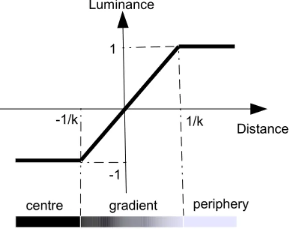
Figure 3.2: The luminance transition model of parameter k.

• tu and tv are the coordinates of the ellipse centers; these are the two

para-meters that represent keypoint coordinates.

3.2.2 Intensity model

The model assumes constant intensity in the disk center and in the periphery with a linear transition between both. For the given luminance levels L1 at the center of the patch and L₂ at its periphery, assuming the patch is darker than background

L1 < L2, the luminance transition is represented by three line segments as shown

on Figure 3.2 with the gradient part being linear with slope k. The distances −1_k and 1_k define the border of the center, gradient and periphery areas.

For each pixel point (x0, y0) there is a model point (x, y) obtained by (3.4) which lies at distance dc =

p

x2_{+ y}2 _{from model’s center for a circle with normalized} radius 1; if we place the origin at distance 1 from circle center as displayed on Figure 3.2, the model point distance will be defined as d = d_c− 1. The model point has its corresponding normalized luminance level ˜L(x0, y0) (normalized on the

(31)

interval [ ˜L1 = −1, ˜L2= 1]) which is assigned depending on the interval: ˜ L(x0, y0) =        −1, d ≤ −1_k kd, −1 k < d < 1 k 1, d ≥ 1_k (3.5)

The denormalization of ˜L(x0, y0) is to be done:

L(x0, y0) = L₁+ ˜

L(x0, y0) + 1

2 (L2− L1) (3.6)

Therefore, there are three parameters which describe the color model and which will be used in the minimization process:

• L1 - luminance level at the center area of the patch • L2 - luminance level at the periphery

• k - slope which defines the transition from the center to periphery areas

3.2.3 Parametric model estimation through minimization

Levenberg-Marquardt algorithm (LMA) is chosen to minimize the sum of squared differences of the gray levels between each pixel (x0, y0) of the elliptic patch in the image I and corresponding point (x, y) obtained by (3.4) of the theoretical CCD model with intensity L as in (3.6). The model is represented by a set of parameters {h₁, h2, θ, tu, tv, k, L1, L2} that comprises both geometry and color properties. The following distance function is to be minimized by the LMA:

arg min h1,h2,θ,tu,tv,k,L1,L2 w X x0 h X y0 (I(x0, y0) − L(x0, y0))2. (3.7)

After the minimization process is terminated, among the set of obtained model parameters, there is a sub-pixel center coordinate (tu, tv) which represents a

key-point.

3.2.3.1 Parameter initialization

Given three channels of the image, the very first step is to estimate initial position of each disk and the size of its enclosing sub-image. This is done by proceeding: Step 1. Binarization of each channel.

Step 2. Finding connected components of a black color for each binarized channel. Step 3. Calculating moments for each component i:

(32)

3.2. Sub-pixel keypoint detection 19

(b) compactness measure Ci = 4πS_P2i

i

, where Pi is a closed curve of the

con-nected component area Si,

(c) centroid (tiu, tiv).

Step 4. Noise elimination by meeting the conditions:        min(r_i_x, riy) > 8 1 − δ ≤ Ci≤ 1 + δ, δ ∈ [0.2, 0.4] Si ∈ {S}f req, (3.8)

where {S}f req is a histogram area with most frequent connected component

sizes

As a result we obtain initial positions of each disk (tiu, tiv) and its enclosing

sub-image with size w_i = h_i= r_i5₂, where r_i= 1₂(r_i_x+ r_i_y).

The initialization of other geometric parameters h₁, h₂ and θ is done with help of principle component analysis. If we represent an ellipse by its covariance matrix

Cov = " (σx)2 σxy σxy (σy)2 # , (3.9)

where σ_x- one-sigma uncertainty in x direction, σ_y - in y direction and σ_xy - covari-ance between x and y. The axes and their lengths are represented by eigenvectors and eigenvalues accordingly. We are interested in eigenvalues in order to initialize

h1 and h2. Given matrix Cov, a characteristic equation can be written:

|Cov − λI| = " (σ_x)2 σxy σxy (σy)2 # − " λ 0 0 λ # = 0. (3.10)

The determinant calculation will lead to a quadratic equation:

λ2− ((σ_x)2+ (σ_y)2)λ + (σ_x)2(σ_y)2− (σ_xy)2 = 0, (3.11)

which has roots

λ1,2= (σ_x)2_{+ (σ} y)2± q ((σ_x)2_{+ (σ} y)2)2− 4((σxσy)2− (σxy)2) 2 (3.12)

The lengths of the ellipse axes are square root of eigenvalues λ₁, λ₂of covariance matrix Cov and since parameters h₁ and h₂ represent semi-axes, we can initialize them as h1= √ λ1 2 h2= √ λ2 2 (3.13)

(33)

The counter-clockwise rotation θ of the ellipse then can be deduced from the first column of 3.10, which also means [cos θ sin θ]T, and therefore we can write

θ = atan2((σx)2− λ1, σxy). (3.14)

The other model parameters are initialized: {k = 2, L₁ = black∗, L2 = white∗}, where black∗, white∗ are global maximum and minimum intensities for the given sub-image [wi× hi].

3.2.3.2 Error

The element of an error vector E = (e_(0,0), e_(0,1), · · · , e_(w,h)) for a set of pixels of the image with size w × h of the elliptic patch is given by:

e(x0_,y0₎= I(x0, y0) − L(x0, y0) (3.15)

3.2.3.3 Jacobian matrix

The Jacobian matrix is determined as a matrix of all first-order partial derivatives of the vector function {λ₁, λ2, θ, tu, tv, k, L1, L2} with respect to data vector. The generic formulations for the geometry variables (not including k, L1, L2 variables) for a given image pixel (x0, y0) are:

∂e(x0_,y0₎ ∂• = − ∂L(x0, y0) ∂• ∂L(x0, y0) ∂• = 1 2(L2− L1) ∂ ˜L(x0, y0) ∂• ∂ ˜L(x0, y0) ∂• = k ∂d ∂•, (3.16)

where the formulas of partial derivatives ∂ ˜L(x 0_{, y}0₎

∂• for each variable are given only

for the gradient interval −1_k < d < 1_k (since the derivatives will be zeros at periphery and at the center areas, see (3.5)), and further on the derivatives are shown only for this interval.

The derivatives for color variables k, L1, L2 are straightforward:

∂e(x0_,y0₎ ∂• = − ∂L(x0, y0) ∂• ∂L(x0, y0) ∂k = (L2− L1) d 2 ∂L(x0, y0) ∂L1 = 1 − ˜ L(x0, y0) + 1 2 ∂L(x0, y0) ∂L2 = ˜ L(x0, y0) + 1 2 (3.17)

(34)

3.3. Keypoint ordering 21

Figure 3.3: Example of the pattern image.

The formulas of partial derivatives ∂d

∂• for each geometric variable are: ∂d ∂• = 1 d(x ∂x ∂• + y ∂y ∂•) ∂x ∂λ1 = (x0− t_u) cos θ, ∂y ∂λ1 = (x0− t_u) sin θ ∂x ∂λ2

= −(y0− t_v) sin θ, ∂y

∂λ2 = (y0− t_v) cos θ ∂x ∂θ = −(λ1(x 0_{− t} u) sin θ + λ2(y0− tv) cos θ), ∂y ∂θ = (λ1(x 0_{− t} u) cos θ − λ2(y0− tv) sin θ) ∂x ∂tu = −λ₁cos θ, ∂y ∂tu = −λ₁sin θ ∂x ∂tv = λ₂sin θ, ∂y ∂tv = −λ₂cos θ (3.18) The resulting Jacobian matrix has the form:

J =        ∂e(0,0) ∂λ1 ∂e(0,0) ∂λ2 · · · ∂e(0,0) ∂L1 ∂e(0,0) ∂L2 ∂e(0,1) ∂λ1 ∂e(0,1) ∂λ2 · · · ∂e(0,1) ∂L1 ∂e(0,1) ∂L2 .. . . .. ∂e(w,h) ∂λ1 ∂e(w,h) ∂λ2 · · · ∂e(w,h) ∂L1 ∂e(w,h) ∂L2        (3.19)

3.3 Keypoint ordering

The algorithm is fully automatic and does not require any user interaction. We aim at a set of very simple steps that help to order keypoints. The pattern sample is displayed on Figure 3.3

In order to process the set of keypoints to the algorithm, it is important to order them exactly same way as pattern keypoints are, for example from top to bottom column-wise. Simple sorting techniques such as ordering according u and then v

(35)

coordinate may not be efficient since we deal with the image of the pattern which was rotated, translated and then projected into camera image. The simplest way was to determine approximate homography Happ using match of corner keypoints

of the image and the pattern, and then order the rest of image keypoints with help of H_app. Therefore, we are interested in selecting the four ellipses that are located at the corners of the calibration pattern and then putting them in correspondence with the corners of model pattern. If we are able to estimate this transformation, then we can easily estimate the correspondence for the rest of the points. This is carried out by means of homography.

The similar idea is usually applied in human-assisted semi-automatic environ-ment where a user selects the four corners and the algorithm manages to do the rest, for example, Matlab Calibration Toolbox [BOUGUET 2000]. Our goal is to have fully automatic software.

The principle for determination of corners from a given set of keypoints is dis-played in Figure3.4. We followed these steps to order all the keypoints:

1. For each of the keypoint c (potentially corner) do:

• find its first three neighbours n1, n2and n3 based on Euclidean distance; • calculate the angles ∠n1cn2, ∠n1cn3, ∠n2cn3 and pick the maximum ∠max = ∠ni1cni2 with i1 and i2 corresponding keypoint indices that satisfy maximum angle condition;

• if the angle is more than 180◦ then c is not a corner;

• otherwise for all the rest of the keypoints {n_i}_{i=3,··· ,N}, make sure they are located within the maximum angle_∠ni1cni2 (within small tolerance

ε, for example, 2◦) and if this condition holds, c is a corner:

∠ni1cni2 > ∠nicni1− ε

∠ni1cni2 > ∠nicni2− ε

(3.20)

2. Sort the four corners by coordinate - firstly by u, then by v.

3. Calculate approximate homography Happusing correspondence of corner

key-points c₁, c₂, c₃, c₄, and corresponding pattern corner keypoint locations. 4. Sort all the keypoints same way as they are sorted for the pattern by

calcu-lating approximate location of the keypoint in image xapp= HappX and then

identifying the closest keypoint x to xapp.

3.4 Sub-pixel ellipse center detection accuracy

Experiments are performed to measure the ellipse center detection accuracy at different ellipse sizes against noise and aliasing, and also against different angles

(36)

3.4. Sub-pixel ellipse center detection accuracy 23

n1 _n2

n3 c

Figure 3.4: Defining the corner keypoint: when the maximum angle_∠n₁cn3between corner’s c first three neighbours n₁, n₂, n₃ stays maximum for the rest of the keypoints (within small tolerance) and at the same time less than 180◦.

An object

Digital image

Sub-sampling

Digitizing

+ Noise

+ Smooth

Camera

Figure 3.5: Digitizing of the pattern.

of view of the circle. The synthetic data was generated according a principle of digitizing shown on Figure 3.5.

Synthetic disk (filled circle) 8-bit images were generated on a large image of size

W × W pixels (W = 1000 for the first set and W = 2000 for the second), which was

blurred, downsampled and finally Gaussian noise was added. Subpixel disk center location is used as ground truth and compared to detected disk center.

Each set includes four 8-bit images with a disk on each of a different radius size. That is, an ellipse {x, y} is drawn with the fixed center (xc, yc), radius R

and rotation angle ϕ (fixed to 30◦) along z axis and changing angle of view θ as described: ((x − x_c) cos ϕ − (y − y_c) sin ϕ)2 R2 + ((x − x_c) sin ϕ + (y − y_c) cos ϕ)2 (R cos θ)2 ≤ 1, (x_c, yc) = (0.5W + δx, 0.5W + δy), R = nW 2 , (3.21)

where (δx, δy) are shifts from image center for x, y directions, and n =

[0.45, 0.6, 0.75, 0.9] is assigned so that to see if the ratio between image area and disk area influences the detection accuracy.

(37)

0 0.5 1 1.5 2 2.5 3 3.5 4 0 0.002 0.004 0.006 0.008 0.01 Noise (Variance) Error (Pixels) R/s=13 R/s=15 R/s=19 R/s=23

(a) Gaussian noise, W = 1000

0 5 10 15 20 0 0.01 0.02 0.03 0.04 0.05 Blur (Std dev) Error (Pixels) R/s=13 R/s=15 R/s=19 R/s=23 (b) Aliasing, W = 1000 0 0.5 1 1.5 2 2.5 3 3.5 4 0 1 2 3 4 5 6 7x 10 −3 Noise (Variance) Error (Pixels) R/s=25 R/s=30 R/s=38 R/s=45 (c) Gaussian noise, W = 2000 2 4 6 8 10 12 14 16 18 20 0 0.01 0.02 0.03 0.04 0.05 0.06 0.07 Blur (Std dev) Error (Pixels) R/s=25 R/s=30 R/s=38 R/s=45 (d) Aliasing, W = 2000

Figure 3.6: Keypoint detection precision performance for normal angle view θ = 0◦ with subsampling rate s = 20, original image resolution W and subsampled circle radii R_s, pixels.

The ground-truth circle centers for each sub-sampled image are found:

(x_g.t, yg.t) = (0.5 W s + δx s, 0.5 W s + δy s), (3.22)

with s being a downsampling rate (s = 20 for both image sets). Figure 3.6 and Figure 3.7 show the performance of the algorithm against Gaussian noise level (median error out of 100 iterations) and amount of aliasing for different disk radii (the view angle θ is set to 0◦ on the first figure and 55◦ on the second). Similar experiments were performed for other view angles, up to 70◦ and it was found that error always has the same tendency as in shown figures.

3.5 Conclusion

The described algorithm allows automatic keypoint detection and ordering of the circled pattern. From the graphs presented at experiment section it can be also concluded:

1. In all the cases the average error is less than 0.05 pixels, even for small disk radius (11 pixels). And considering the fact that ratio of the disk area and its

(38)

3.5. Conclusion 25 0 0.5 1 1.5 2 2.5 3 3.5 4 0 0.002 0.004 0.006 0.008 0.01 0.012 0.014 Noise (Variance) Distance (Pixels) R/s=13 R/s=15 R/s=19 R/s=23

(a) Gaussian noise, W = 1000

0 5 10 15 20 0.02 0.03 0.04 0.05 0.06 0.07 Blur (Std dev) Error (Pixels) R/s=13 R/s=15 R/s=19 R/s=23 (b) Aliasing, W = 1000 0 0.5 1 1.5 2 2.5 3 3.5 4 0 0.002 0.004 0.006 0.008 0.01 Noise (Variance) Error (Pixels) R/s=25 R/s=30 R/s=38 R/s=45 (c) Gaussian noise, W = 2000 2 4 6 8 10 12 14 16 18 20 0.015 0.02 0.025 0.03 0.035 0.04 0.045 0.05 Blur (Std dev) Error (Pixels) R/s=25 R/s=30 R/s=38 R/s=45 (d) Aliasing, W = 2000

Figure 3.7: Keypoint detection precision performance for θ = 55◦ angle view with subsampling rate s = 20, original image resolution W and subsampled circle radii

R

(39)

enclosing image area has little impact on the precision detection, allows us to pack more keypoints in a given pattern area.

2. The angle of view has little influence on precision even for large angles, which means the detection stays robust even when pattern plane is viewed from a large angle of view (here we don’t consider perspective bias which is a subject in Chapter 5, but rather affine transform of the elliptic parameters).

3. As expected, the error increases linearly with noise level, but remains constant under aliasing. This is important because in a Bayer pattern image, red and blue channels are notoriously aliased. Figure 3.6 (b,d) and Figure 3.7 (b,d) show that this does not affect the disk center detection.

(40)

Chapter 4

High-precision correction of

lateral chromatic aberration in

digital images

Nowadays digital image sensor technology continues to develop much faster than optical technology for imaging systems. The result quality loss is due to lateral chromatic aberration and it is becoming more significant with the increase of sensor resolution. For the sake of higher performance and lighter lens systems, especially in the field of computer vision, we aim to find new ways to overcome resulting image quality limitations.

This chapter demonstrates a robust method to minimize the lateral chromatic aberration, recovering the loss of image quality by using a single circled pattern image. Different series of tests and measures are used to validate the algorithm. For the performance evaluation we used both synthetic and real data.

The primary contribution of this work is an effective algorithm to robustly correct lateral chromatic aberration through color planes warping. We aim at high precision (largely sub-pixel) realignment of color channels. This is achieved thanks to two ingredients: high precision keypoint detection, which in our case are circle centers, and more general correction model than what is commonly used in the literature, radial polynomial. The setup is quite easy to implement, requiring a pattern of black disks on white paper and a single snapshot.

We perform the error measurements in terms of geometry and of color. Quantit-ative results on real images show that our method allows alignment of average 0.05 pixel of color channels and residual color error divided by a factor 3 to 6. Finally, the performance of the system is compared and analysed against three different software programs in terms of geometrical misalignments.

Keywords Chromatic aberration, image warping, camera calibration, polynomial model, image enhancement

Contents

4.1 Introduction . . . . 29

4.2 Calibration and correction . . . . 32

4.3 Experiments . . . . 35

(41)

4.3.2 Visual improvement for real scenes . . . 46

4.3.3 Experiments with compact digital cameras . . . 46

Towards high precision internal camera calibration

HAL Id: tel-01133601

https://pastel.archives-ouvertes.fr/tel-01133601

Victoria Rudakova

To cite this version:

Thèse de doctorat

de l’UNIVERSITÉ PARIS EST

Vers l’étalonnage interne de caméra à haute précision

PHD thesis

of UNIVERSITÉ PARIS EST

Towards high precision internal camera calibration

Acknowledgements

Contents

Chapter 1

Introduction - version française

1.1

Correction de l’aberration chromatique

1.2

Extraction de caméra matrice

1.3

Les chapitres de la thèse

1.4

Les contributions principales

Chapter 2

Introduction

2.1

Chromatic aberration correction

2.2

Camera matrix extraction

2.3

The thesis chapter by chapter

2.4

Main contributions

Chapter 3

Robust and precise feature

detection of a pattern plane

3.1

Introduction

3.2

Sub-pixel keypoint detection

An object

Digital image

Digitizing

+ Noise

+ Smooth

Camera

An object

Digital image

Sub-sampling

Digitizing

+ Noise

+ Smooth

Camera

3.3

Keypoint ordering

3.4

Sub-pixel ellipse center detection accuracy

An object

Digital image

Digitizing

+ Noise

+ Smooth

Camera

3.5

Conclusion

Chapter 4

High-precision correction of

lateral chromatic aberration in

digital images